DDTree: A Hybrid Deep Learning Model for Real-Time Waterway Depth Prediction and Smart Navigation

Abstract

Timely and accurate depth estimation of a shallow waterway can improve shipping efficiency and reduce the danger of waterway transport accidents. However, waterway depth data measured during actual maritime navigation is limited, and the depth values can have large variability. Big data collected in real time by automatic identification systems (AIS) might provide a way to estimate accurate waterway depths, although these data include no direct channel depth information. We suggest a deep neural network (DNN) based model, called DDTree, for using the real-time AIS data and the data from Global Mapper to predict waterway depth for ships in an accurate and timely way. The model combines a decision tree and DNN, which is trained and tested on the AIS and Global Mapper data from the Nantong and Fangcheng ports on the southeastern and southwestern coast of China. The actual waterway depth data were used together with the AIS data as the input to DDTree. The latest data on waterway depths from the Chinese maritime agency were used to verify the results. The experiments show that the DDTree model has a prediction accuracy of 91.15%. Therefore, the DDTree model can provide an accurate prediction of waterway depth and compensate for the shortage of waterway depth monitoring means. The proposed hybrid DDTree model could improve marine situational awareness, navigation safety, and shipping efficiency, and contribute to smart navigation.

1. Introduction

Water transport is the main transportation mode for the ever-increasing volume of international trade. The high capacity, cost savings, low energy consumption, and advances in the development of waterborne transportation make it the preferred mode for long-distance trade, when compared to other means of transport. Based on the latest report of the International Maritime Organization (IMO) [1], 90% of goods are currently transported by shipping. Maritime vessel traffic differs from ground-based traffic because of the complexity of rapidly changing the direction of the ships on the water [2]. In order to ensure that the ship passes safely through the waters, the water depth should be greater than the sum of the draft of the ship and surplus under keel clearance (UKC) [3]. Due to the lack of real-time monitoring means, there are often economic losses due to excessive ship loading, resulting in ship stranding and port obstruction. In this context, the development of new methods for increasing situational awareness and achieving smart maritime navigation is highly relevant [4].

Obtaining actual water depths, however, is difficult because the water depth changes constantly. Water depth data that are found in the electronic chart display and information system (ECDIS) and water-way area maps, therefore, are not accurate, which may cause ships to be stranded, collide, and hit rocks. Such accidents can result in serious casualties and property loss, and may even cause serious damage to regional transportation. For example, in the period from 2013 to 2014, the reef accidents in the Yangtze River navigation channel accounted for 10% of all accidents in the Yangtze River, and the proportion of all kinds of vessel accidents on the Yangtze River was 17% [5]. The total number of accidents caused by insufficient navigation depth was 27%. Therefore, having accurate and timely knowledge of water depth data is of great significance to safe navigation. The problem is especially relevant in the context of Internet-of-Things (IoT) solutions for smart ships [6], connected ships [7], and next generation marine data networks [8] in which the problems of quality of service and environmental awareness arise [9].

In water transport, the water depth of a channel refers to the vertical distance from the water level to the bed of a waterway channel. For a local section of a waterway, it usually refers to the vertical distance from the water level to the bed at the shallowest part of a channel. Safe water depth and the depth of water needed for a ship to pass safely acts as a guide for route planning and safe navigation of ships. The bottom of the shallow channel can be heavily silted under the hydrological conditions of wind, waves, and currents. A review of the literature reveals two broad approaches for obtaining the water depth of a waterway: (1) monitoring of the water depth with sonar and other detection devices, and (2) time-delay acquisition and processing of underwater acoustic signals to calculate the waterway depth.

At present, the prediction methods in ship transportation focus on short-term traffic flow prediction, and traffic congestion forecasting. The predictions of depth in waterways are obtained through satellite remote sensing images and real-time sensors; for instance, when performing monitoring of oil spills [10]. Since almost all in-flight vessels are equipped with automatic identification systems (AIS), the analysis of full AIS data and the development of deep learning models could support the improved prediction of waterway depth.

In this paper, a hybrid decision tree-deep neural network (DDTree) model is constructed to predict safe waterway depths for ships to increase the precision and timeliness of the waterway depth data and provide references for safe marine navigation and route selection. The rest of this paper is organized as follows. In Section 2, the conceptual model for the analysis of the actual waterway depth data (from Global Mapper) and the AIS data are introduced, and the proposed DDTree model is presented. In Section 3, the results for prediction of waterway depth are presented and the model’s performance is analyzed. Finally, Section 4 presents the conclusions of the paper.

2. Related Work

In the field of waterway transportation, current research related to the prediction of water traffic focuses on progressive water prediction of depth. Big data collected in real time by automatic identification systems (AIS) might provide a way to estimate accurate real-time waterway depths, but these data include no direct channel depth information [11]. The large volume ship AIS data are widely used in navigation. In addition, the wide application of GNSSs (global navigation satellite systems) also provides technical support and a safety guarantee for navigation. Therefore, by employing the data-mining techniques on big data from AIS and GNSS, the waterway depth can be predicted. For example, Su et al. [12] proposed using multi-spectral satellite images to predict water depth change along a waterway. In order to enhance the accuracy of water prediction of depth, Kang et al. proposed a differential dynamic positioning algorithm based on GPS/Beidou which realizes middle precision based on low cost equipment [13]. Kamil Maciuk analyzed the accuracy of static GNSS measurements according to the number of visible satellites, based on different minimal elevation cutoff angles [14]. Hsin-Hung Chen et al. proposed two synthetic models for sound-speed profiles, one linear and the other bilinear [15]. Similarly, EL-Hattab [16] analyzed critical issues in GPS precise positioning. Mamoun F. Abdel-Hafez et al. addressed the problem of estimating the measurements’ noise statistics of the Global Positioning System (GPS) using the autocovariance least squares technique [17]. Younis et al. [18] proposed a method for predicting the depth of water in a rough composite channel. Shiri et al. [19] proposed a wavelet and a fuzzy neural network model to estimate the depth of groundwater. Prediction of waterway depth can be a part of larger models focused on avoiding marine traffic accidents and ship collision. For example, Wang et al. [20] applied short-time space-time analysis of the AIS data to analyze in-land water ship collisions. Vodas et al. [21] proposed a ship accident prediction and judgment model based on the AIS data. Li et al. [22] proposed a method to improve the AIS data collection equipment. Through the detailed analysis of the data received by the AIS receiver in Skynet 3’s debugging stage, receiving capability was improved. Mulyadi [23] proposed a Bayesian network-based model for assessing the frequency of ship sinking accidents. Similarly, Li et al. [24] used generalized Bayesian inference and the Dempster’s rule to recognize the patterns of ship traffic from historical AIS data. Salmalian et al. [25] predicted ship squat behavior in shallow water depending upon waterway depth. They used the group method of data handling (GMDH) neural networks and an adaptive network-based fuzzy inference system (ANFIS) with good results. Niu et al. [26] used the feed-forward neural network (FFNN) and support vector machine (SVM) classifiers to infer ship location from acoustical data in a deep waterway channel. Bannari et al. [27] suggested an approach for bathymetric mapping of shallow water of Arabian Gulf near Bahrain using the kriging procedure. Kim and Lee [28] proposed the ship traffic extraction neural network (STENet) to forecast the maritime traffic of the caution area, which represented an increased risk for ships, due to things such as berth limitations. Jeong et al. [29] performed multi-criteria route planning using the AIS data while considering waterway depth (in the navigable area) as one of risk factors and criteria for optimization. Rong et al. [30] adopted the kernel density estimation-based method for mining ships’ behaviors from the AIS data. Xin et al. [31] proposed a ship traffic simulation model for in the Xiazhimen waterway for analyzing the statistical characteristics of ship traffic. Zhang et al. [32] analyzed the spatial-temporal dynamic of traffic in port waterways while using the AIS data. Finally, Yang et al. [33] overviewed and summarized main contributions of the AIS data for marine navigation safety. Machine learning approaches has been used in addressing challenges in many fields, such as medical and engineering. For example, Gianni D’Angelo et al. presented a robust approach to the optimal policy of autonomous space systems modeled via Markov decision process (MDP) from the values assigned to its transition probability matrix [34]. In the medical field, Gianni D’Angelo et al. presented a proposal for distinguishing between bacterial and viral meningitis using genetic programming and decision trees [35]. Machine learning methods are also widely used in prediction problems, and have achieved good results in problems such as weather forecasting and ocean wave prediction.

3. Domain Analysis and Definition of Conceptual Model

3.1. Data

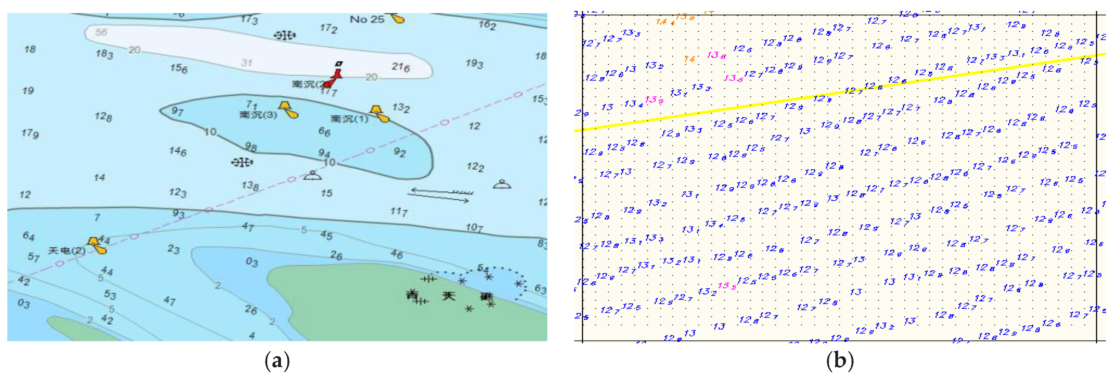
Waterway depth is the vertical distance from the water surface to the bottom (seafloor) of a waterway. At present, the waterway depth data can be extracted from the electronic charts visualized cartographically, as shown in Figure 1a. In addition to the ECDIS charts, the berth map also presents the waterway depth data. Unlike an electronic chart, the berth map divides the watercourse according to the geographical position, displaying waterway depth information from berths, as shown in Figure 1b. Figure 1a,b illustrates two waterway depth data acquisition methods. The waterway depth data can be obtained from ECDIS or from berth map. On the other hand, the prediction of unknown depth data from the available depth-related data is the main research goal of this paper.

Figure 1. Waterway depth data (ground truth) from: (a) electronic chart display and information system (ECDIS) depth data; (b) berth map of depth.

The AIS data represent the static data and the dynamic data of the ships. The dynamic data have information such as Maritime Mobile Communication Service Identification (MMSI) number, latitude and longitude, speed/course over ground, steering rate, and headings [36]. The static data include inherent information about a ship, such as the length, the breadth, the maximum draft, and the type. Table 1 shows an example of the AIS data.

Table 1. Fragment of automatic identification system (AIS) data: Maritime Mobile Communication Service Identification (MMSI) code is a unique identifier for ships. SOG is the speed of the ship to the ground, COG is the heading of the ship to the ground, and UTC is the current time.

MMSI	Longitude/(°)	Latitude/(°)	SOG/(n Mile/h)	COG/(°)	UTC
413769173	114.3079	30.58732	6.0	33.8	2016/4/23 1:08
413769173	114.3102	30.59013	6.0	31.6	2016/4/23 1:10
413769173	114.3113	30.59168	6.1	34.0	2016/4/23 1:11
413769173	114.3124	30.59305	6.1	32.0	2016/4/23 1:12

Since there are missing points in AIS data, the longitude and latitude data must be imputed by the data interpolation method, making the water depth information more complete. The cubic spline interpolation method obtains waterway depth data corresponding to different latitude and longitude points in the waterway, and the obtained waterway depth data are integrated according to the longitude and latitude values and the AIS data of the waterway, so that the depth data and the AIS dynamic data are combined with static data.

3.2. Conceptual Model

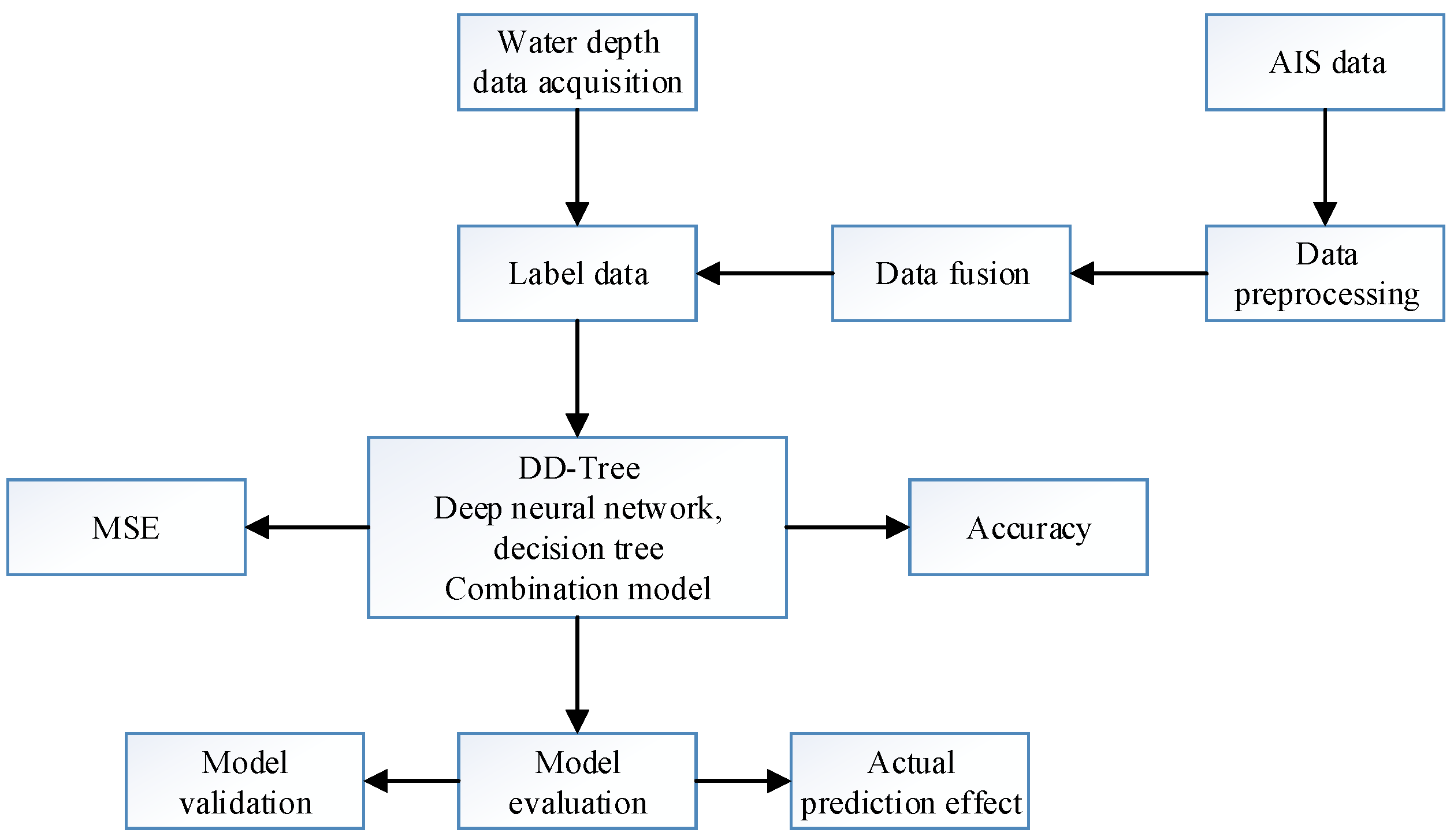
In order to achieve the prediction of waterway depth, we have designed, evaluated, and verified the proposed DDTree model. First, the AIS data must go through preprocessing and abnormal data detection and other methods to remove redundant and abnormal data (see Figure 2). There are many errors, omissions, and noises in AIS data. The use of erroneous data for calculation or analysis may lead to a wrong conclusion. Therefore, it is critical to preprocess the data and delete the obvious noise information, such as latitude 89°, negative longitude, and the data whose MMSI is not nine digits. At the same time, some redundant information should also be deleted; for example, AIS dynamic information has much duplicate data. Then, the AIS data and waterway depth data are combined to build a deep neural network dataset. After training datasets and verification datasets are divided, the network structure is adjusted and the depth data are predicted by the combination of a neural network and a decision tree. Finally, the prediction performance, accuracy, is evaluated.

Figure 2. Flow chart of the waterway depth prediction using the proposed DDTree model.

3.3. Decision Tree

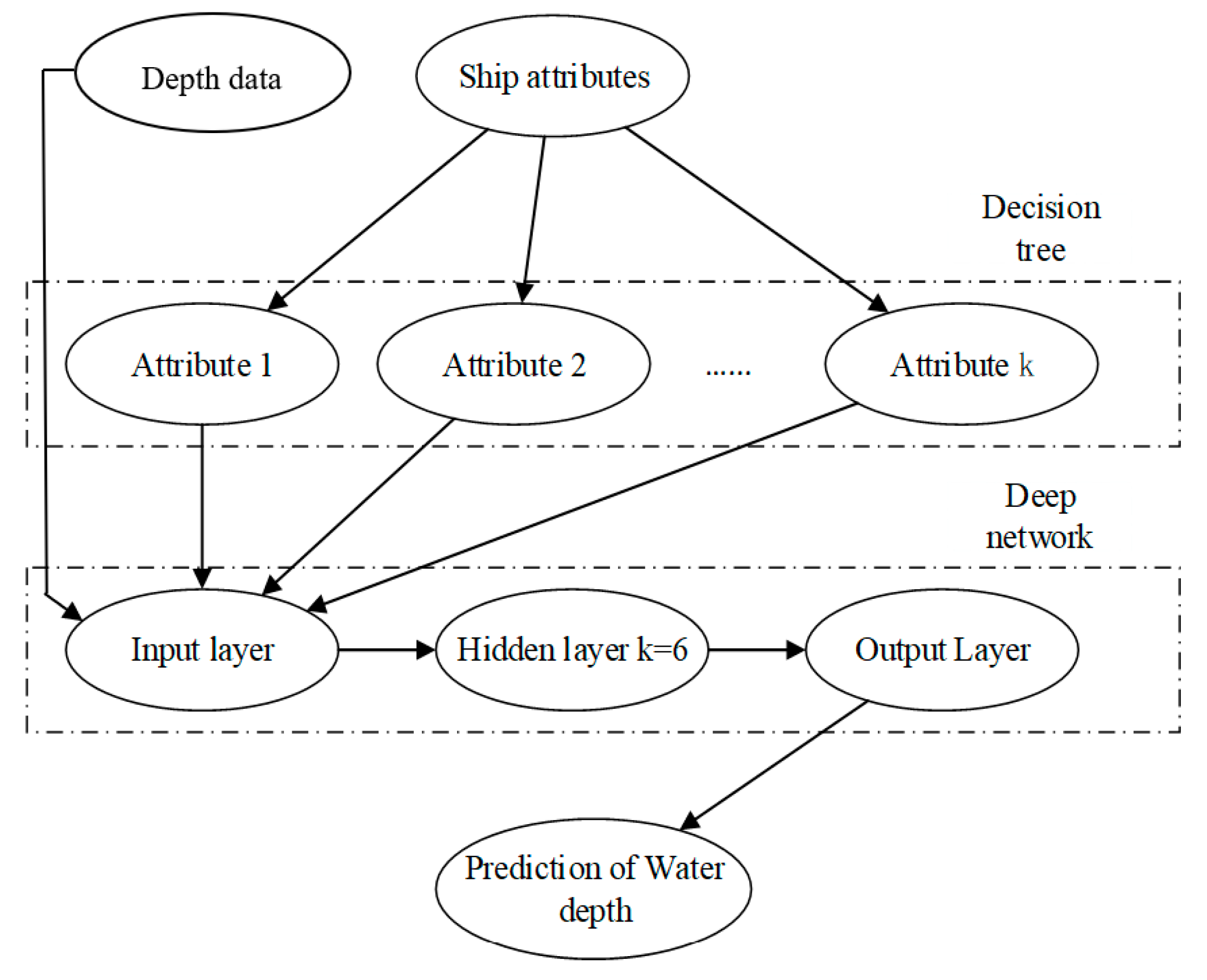
The waterway depth data are predicted through the hybrid model of a decision tree and a deep neural network (DNN). Similar hybrid models combining the models from different subdomains of machine learning have been proven successful for solving various classification and regression tasks [37,38]. The DDTree model is composed of two parts. The decision tree is responsible for selecting different attributes of the static data and dynamic data in the AIS data and selecting the optimal attributes. The DNN is responsible for processing the optimal attributes and generating prediction of waterway depth data.

The waterway depth data are used as supervised data to establish a model for prediction of waterway depth. Figure 3 shows a structure of the hybrid DDTree model. Each non-leaf node in the decision tree represents an attribute of the AIS data with which to judge whether the leaf node belongs to a certain range [39], as is shown in Figure 3. Each branch of a tree represents the output of an attribute over a range of values, which is used to indicate the output value under the corresponding judgment. After evaluating the static and dynamic AIS data in the decision tree, the information gain of different features can be determined, and the correlations between different features and predictive variables can be judged.

Figure 3. The structure of the hybrid DDTree model. Ship attributes are taken from AIS. Depth data for DDTree model input are taken from Global Mapper.

In the root node, we select the attribute in the AIS dataset that accurately decides the waterway depth in the electronic ECDIS chart. The remaining attributes are sorted according to their discriminating value and included in the output branches until reaching the final leaf node of the decision tree. The final left generates the output of the entire decision tree in the DDTree model.

After preprocessing AIS data, the optimal attributes in the AIS data are selected as the input for a DNN using the attribute selection method in the decision tree, by comparing the information gain from each attribute. This avoids selection of data with little influence on prediction, thus making the entire model responsive when estimating waterway depth.

The information entropy $\mathrm{info}\left(\mathit{D}\right)$ must be calculated in order to build a decision tree. Here $\mathrm{info}\left(\mathit{D}\right)$ is the entropy in the training dataset extracted from the AIS data calculated as in Equation (1):

$$\mathrm{info}\left(D\right)=-{\displaystyle \sum }_{i=1}^m{p}_i{log}_2{p}_i$$

(1)

Here ${\mathit{p}}_{\mathit{i}}$ represents the probability that the i-th data category appears in the training tuple.

Assuming that training AIS dataset D is split by attribute A, the information expectation of A to D partitioning is expressed by Equation (2):

$$inf{o}_A\left(D\right)={\displaystyle \sum }_{j=1}^v\frac{\left|D_j\right|}{\left|D\right|}info \left(D_j\right)$$

(2)

We calculate the information gain for the difference between the two datasets by Equation (3):

$$gain\left(A\right)=\mathrm{info}\left(D\right)-{\mathrm{info}}_A\left(D\right)$$

(3)

After calculating the information gain of each attribute, the set of the first $\mathit{k}$ attributes with the largest information gain is selected by the DDTree model as the optimal attribute set $\left({\mathit{X}}_{\mathbf{1}},{\mathit{X}}_{\mathbf{2}},\dots ,{\mathit{X}}_{\mathit{k}}\right)$. The algorithm in the decision tree is used to classify the waterway depth in the entire dataset. Then the decision tree is used to select optimal attributes as inputs for the neural network.

The characteristics of AIS data include the static and dynamic characteristics of ships. Among them, the static characteristics of a ship include the draft of the ship, the length of the ship, and the breadth of the ship. The dynamic characteristics of the ship include data varying momentarily during the movement of the ship, such as the data of the ship’s speed over ground (SOG) and the steering rate. After calculating the information gain of the static and dynamic characteristics of the ship, the optimal number of attribute parameters is set. The static characteristics $\left({\mathit{a}}_{\mathbf{1}},{\mathit{a}}_{\mathbf{2}},\dots ,{\mathit{a}}_{\mathit{n}}\right)$ and the dynamic information gain $\left({\mathit{b}}_{\mathbf{1}},{\mathit{b}}_{\mathbf{2}},\dots ,{\mathit{b}}_{\mathit{n}}\right)$ of the ship are sorted in descending order; the attributes of the first $\mathit{k}$-th ships $\left({\mathit{c}}_{\mathbf{1}},{\mathit{c}}_{\mathbf{2}},\dots ,{\mathit{c}}_{\mathit{k}}\right)$ make the optimal attribute combination. After selecting the optimal attributes, the depth of waterway is predicted by the DNN model.

3.4. Deep Neural Network

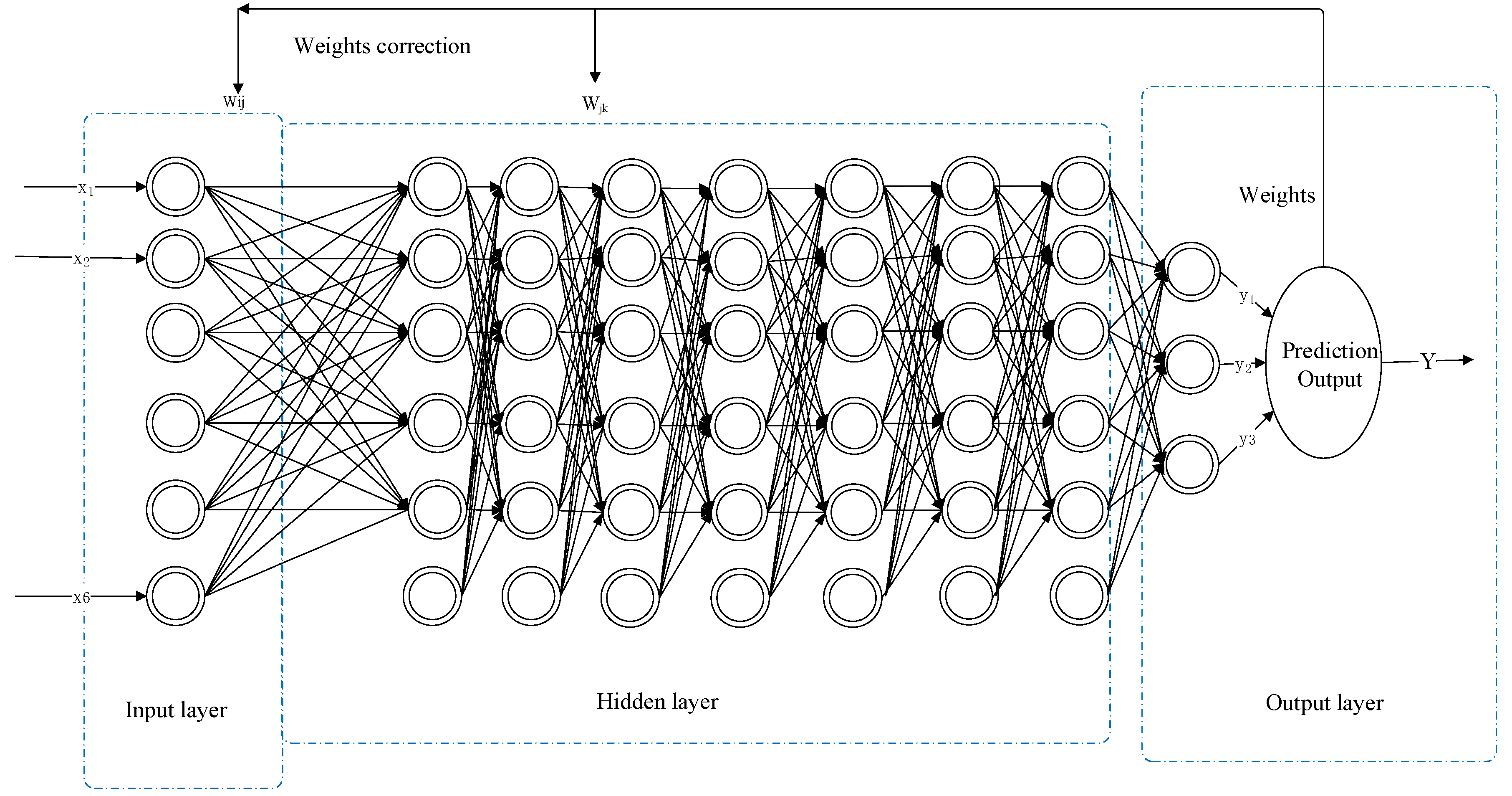
Prediction of waterway depth requires learning through a DNN as a nonlinear input-output model. Figure 4 shows the structure diagram of a DNN, in which the number of hidden layers is seven.

Figure 4. The structure of a deep neural network.

For the prediction of waterway depth, the DNN model uses as the inputs of different AIS attribute data $x=\left(x_1,x_2,\dots ,x_n\right)$ and produces the output y as prediction of depth; $f_1,f_2,\dots ,f_n$ are the activation functions corresponding to each layer in the deep neural network; $\widehat{y}\left(x\right)$ is the output corresponding to each input data. Therefore, for layer l of the network, it can be expressed as Equation (4):

$$f_{w_l,b_l}\left(x\right)=f({\displaystyle \sum }_{j=1}^{N_l}{w}_{lj}{x}_j+b_l)=f\left(w_l^T{x}_l+b_l\right)$$

(4)

where $N_l$ is the number of nodes on the first layer of the network, $w_l\in R^{N_l\times N_{l-1}}$ and $b\in R$, are the weight and bias respectively in the network, and $f_{w,b}$ is the network activation function of each layer.

The optimal attribute is selected by the preceding decision tree model to provide the appropriate input attribute parameters for the DNN. Then, we need to set the initial parameters of the DNN. By iteratively adjusting the weights $w_i$ and offsets ${\theta }_i$ of the DNN, the prediction accuracy is maximized.

For the prediction of the waterway depth of the unknown waterway, DNN aims to predict the waterway depth information of the unknown waterway depth based on the waterway depth data of the known area. The prediction results $y\left(x\right)$ can be expressed as Equation (5):

$$y\left(x\right)={\mathit{x}}_{\mathit{a}+\mathit{h},\mathit{b}+\mathit{h}}^{\mathit{m}}=\left(\begin{array}{l}{x}_{a+h,b+h}^1\\ \dots \\ x_{a+h,b+h}^m\end{array}\right),$$

(5)

where the waterway depth is $x_{a,b}^m$, and the latitude and longitude of the geographical position of the point is (a, b).

For the entire region of the prediction of depth data, the prediction is given by Equation (6):

$${\mathit{x}}^{\mathit{m}}=\left(\begin{array}{l}{x}_{a-h,b-h}^1,\dots ,x_{a+h,b+h}^1\\ \dots \dots \\ x_{a-h,b-h}^m,\dots ,x_{a+h,b+h}^m\end{array}\right)$$

(6)

where n represents points corresponding to different geographic locations, and (a, b) represents the corresponding longitude and latitude.

After preprocessing and analyzing the AIS data, the most important factor for the prediction capability of DNN is to discover the optimal hyperparameter values to achieve the best prediction performance of the entire network. We use the stochastic gradient descent [40] for the network optimization. The range of the network parameters can be specified as Equation (7):

$$\begin{array}{c}f\in \left\{tanh(x),sigmoid\left(x\right),max(x,0)\right\} , \lambda \in \left\{{10}^{-4},{10}^{-2}\right\}, n\in \left\{1,15\right\},N_l\in {\left\{1,200\right\}}^n\\ x_{a+h,b+h}^m=\left(f_1\cdot f_2\cdot f_n\right)x^m, f_l=f\left(w_l^T{x}_l+b_l\right),\end{array}$$

(7)

where λ is the rate of learning, f is the activation function, ${\mathit{N}}_{\mathit{l}}$ is the number of iterations, n is the number of network layers, ${\mathit{x}}_{\mathit{a}+\mathit{h},\mathit{b}+\mathit{h}}^{\mathit{m}}$ is the prediction of depth model structure, and ${\mathit{f}}_{\mathit{l}}$ is the expression of each neural network.

4. Performance Analysis

4.1. Experimental Data

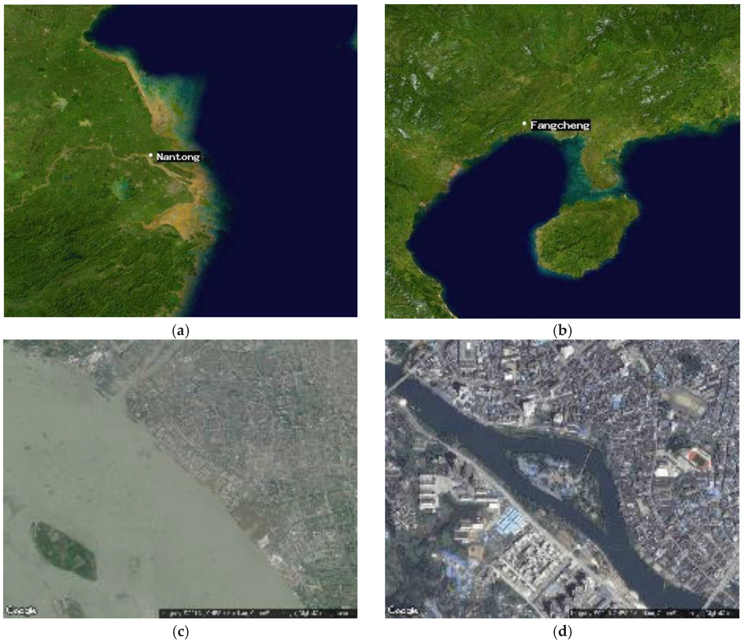
In order to test the proposed hybrid prediction of depth model, the data of Nantong Port in Jiangsu Province of China and Fangcheng Port in Guangxi of China were selected for analysis. Nantong (31° 59′ 32” N, 120° 49′ 46” E) is located near the east Yellow Sea, southwest of the Yangtze River, and it is an important coastal port of China. Nantong has both a natural inland river port and a deep-water coastal port. Fangcheng Port (21° 44′ 58′’ N, 108° 21′ 41′’ E) is a natural river port known as the largest port in western China. Figure 5 shows the satellite images of Nantong Portand Fangcheng Port.

Figure 5. Location of Nantong Port (a) and Fangcheng Port (b) in China, and the satellite maps of Nantong (c) and Fangcheng (d).

The AIS data of Nantong Portand Fangcheng Port were selected for these experiments. The entire AIS dataset contains two parts of the ships’ dynamic data and static data. The waterway depth data used in the prediction of waterway depth model use the depth data provided by the Global Mapper (Blue Marble Geographics, Hallowell, ME, USA) to obtain the dataset corresponding to the latitude, longitude, and depth data through the latitude and longitude matching. Global mapper is the GIS software wherein depths are taken from ECDIS or other bathymetric sources. The waterway depth data at the missing latitude and longitude points are interpolated by three-dimensional interpolation using AIS data latitude and longitude data.

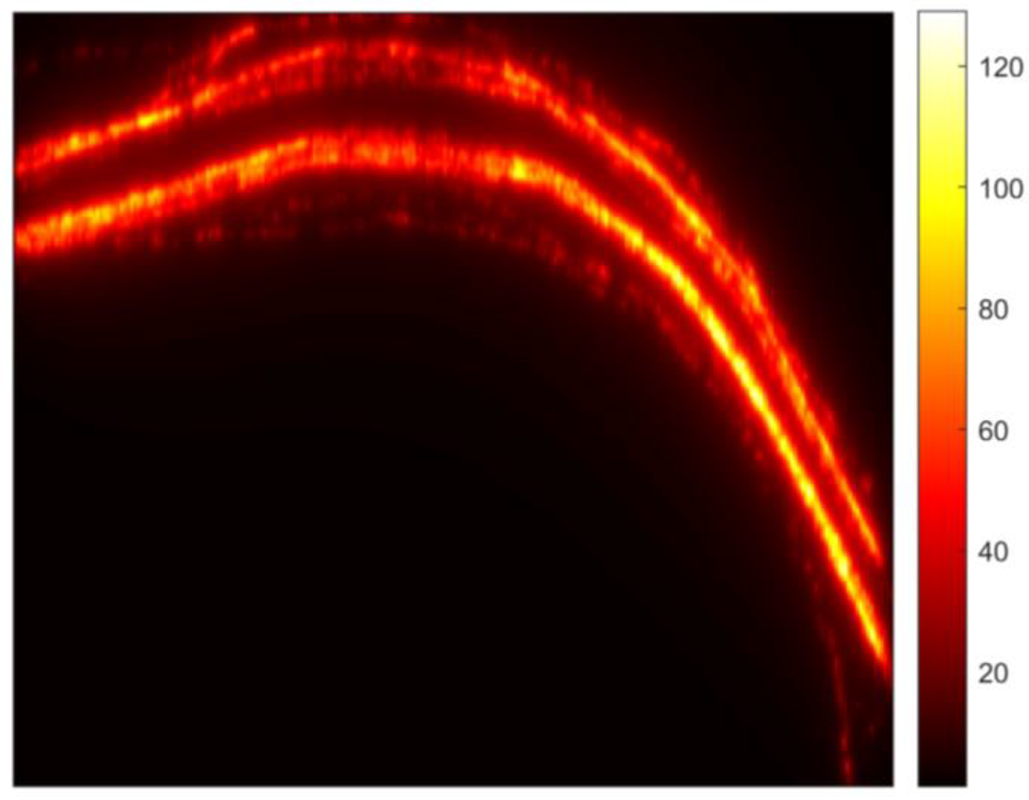
The density map for the Nantong Port dataset showing the most probable positions of ship along the sea fairway is shown in Figure 6.

Figure 6. Density map of ship positions in the Nantong Port AIS dataset.

4.2. Experimental Setting

We selected the AIS data of two waterways in order to predict the waterway depths for Nantong and Fangcheng ports. Through the integration of depth data acquisition and the AIS data, the data of waterway depth and AIS data of the two waterways were obtained as the data sources for this experiment. The total number of data points was 195,742, of which there were 137,006 training data points and 58,718 testing data points. The dataset was divided into training and testing datasets (70% of the data as a training data set, and 30% of the data as a testing data set). These data are used to train the DDTree model to predict the depth of waterway.

Before training, the data were labeled. The data in the waterway area were divided into 25 categories at two-meter intervals from 0 to 50 m depth, and the 26th label was used for depths >50 m. We chose this interval because most of the waterway depth data are around 30 to 40 m, and waterway depth data of less than 30 m and more than 50 m meters are limited.

The hyperparameters of the model (depth of decision tree, activation function, iterations, epochs) were adjusted, and the prediction of waterway depths under different hyperparameter values was recorded. After setting the parameters, the optimal parameters were selected, and the depth data were predicted by the DDTree model and compared with the actual waterway depth (ground truth). Using the model on the test data, the prediction accuracy and the error of the model were calculated.

The input data were classified using a decision-tree classification algorithm. The input parameters were six ship attributes of the dynamic data portion of the AIS data, including speed over ground, ship width, course over ground, draft, and ship steering rate. The processing times of the actual prediction of depth in the Nantong Port and Fangcheng Port using the trained model were 279 s, and 468 s respectively. Table 2 presents the prediction performance to evaluate the decision-tree parameters of the DDTree combination model in relation to the ground truth waterway-depth data. The results we contained with the baseline model, which used a traditional method of data interpolation.

Table 2. Experimental results of the DDTree Model (best value is shown in bold).

k	Depth of Decision Tree	Activation Function	Iteration Step	Epoch	Accuracy
Baseline Model					0.7842
Proposed Model
6	5	sigmoid	100	400	0.8334
6	5	relu	200	600	0.9115
8	7	sigmoid	100	400	0.8652
8	7	relu	200	600	0.8231
10	9	sigmoid	100	400	0.8112
10	9	relu	200	600	0.7992

Table 2 reveals that the DDTree model prediction accuracy was the highest when the value of k was six, the depth of the decision tree was five, the iteration step was 200, and the epoch was 600. After selecting the appropriate neural network parameters, the waterway depth information of the Nantong Port and Fangcheng Port was predicted and analyzed by the model.

4.3. Prediction of Water Depth in Nantong Port

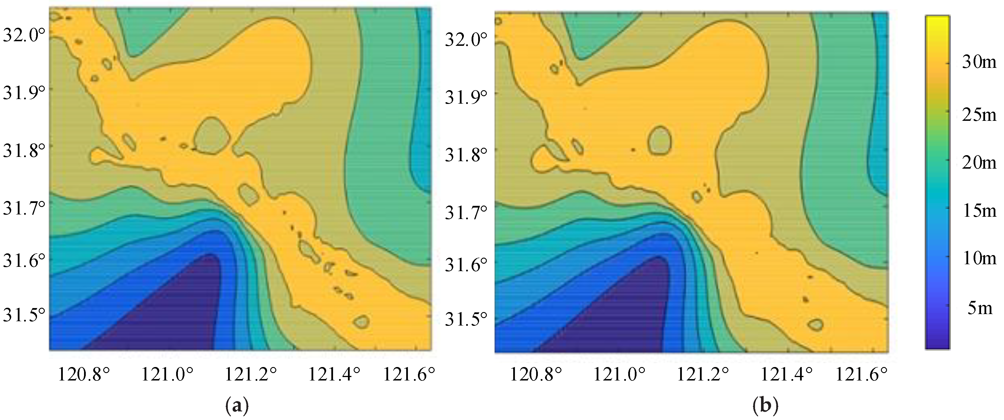
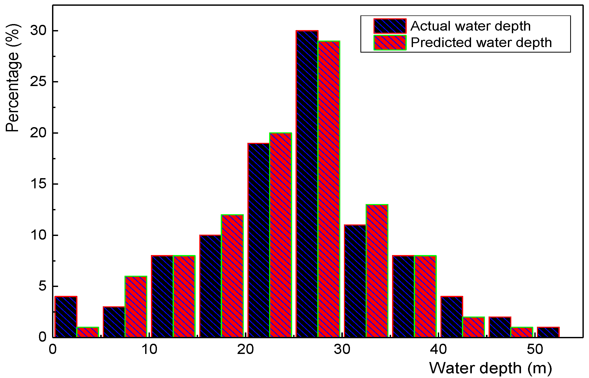
The results of comparative prediction and actual waterway depth results are shown in Figure 7. Figure 7a is an actual distribution map of waterway depth. Figure 7b shows the predicted waterway depth distribution. The distribution histogram of actual and predicted waterway depth of Nantong Port is presented in Figure 8.

Figure 7. Comparison of the results of prediction of waterway depth for Nantong Port: (a) ground truth data, (b) predicted waterway depth.

Figure 8. Actual and predicted water depth data from Nantong Port.

We can see that the proposed model has accurate prediction, and there is an error in the depth data of individual shallows and other locations. The overall prediction accuracy is relatively high and can accurately reflect the distribution of waterway depth in Nantong Port.

4.4. Predicting of Water Depth in Fangcheng Port

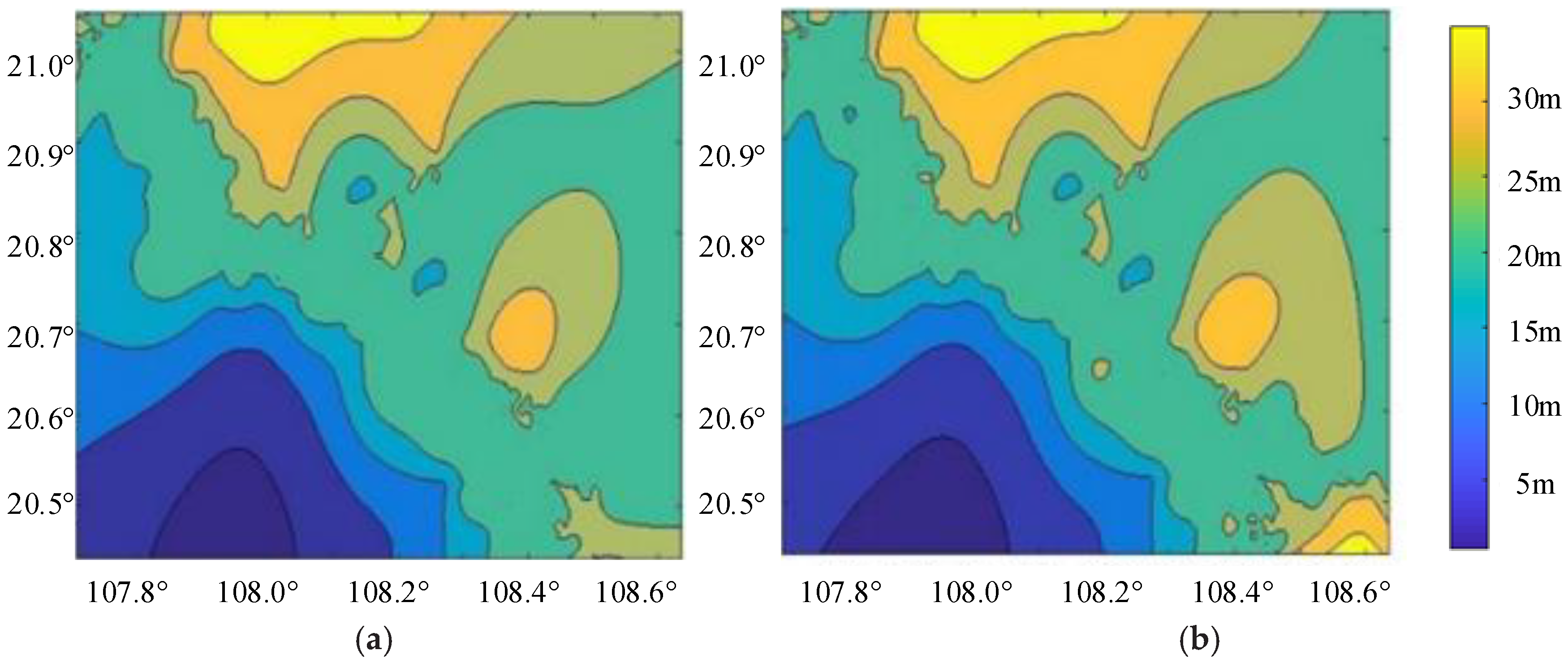
First, the model used the Nantong Port data for the prediction of waterway depth in order to test whether the model had an overfitting situation, verify the ability of the model to predict waterway depth, and assess practicality of the model, but the depth data of other waterways can also be used with this model. Figure 9a,b shows the actual waterway depth and predicted waterway depth distribution for Fangcheng Port using the model trained on the Nantong Port data.

Figure 9. Comparison of the results of prediction of waterway depth for Fangcheng Port: (a) ground truth data, (b) predicted waterway depth.

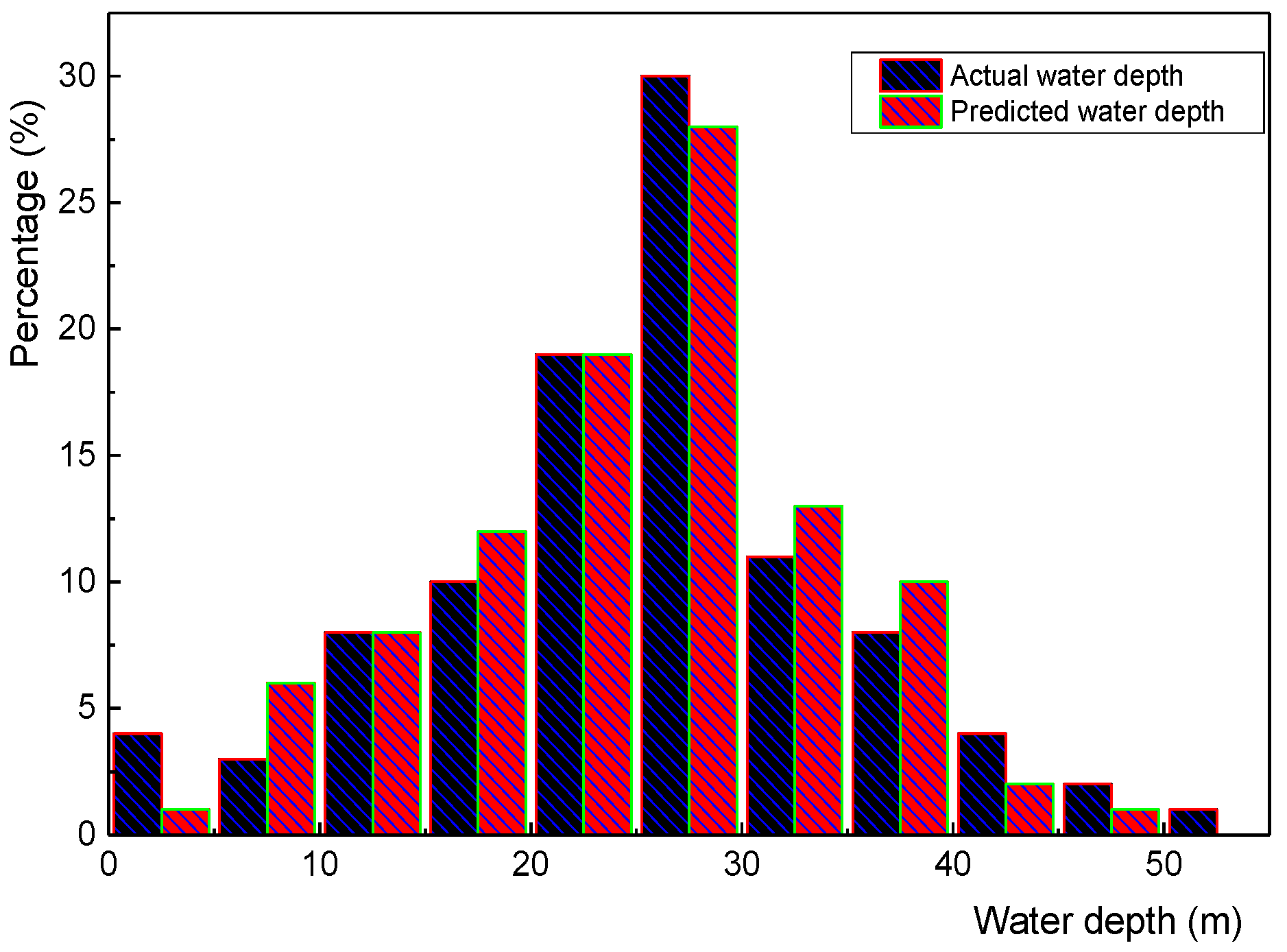
The distribution histogram of actual and predicted waterway depth of Fangcheng Port is shown in Figure 10. This area accounts for the vicinity of the shoal. This part of the waterway depth is complex, leading to unsatisfactory predicting results. The prediction of waterway depth shows that the prediction of depth results of the DDTree model trained using the data from Fangcheng Port have good accuracy, and the predicted waterway depth is consistent with the actual waterway depth, indicating that the model was trained well. The accuracy of the prediction of waterway depth is high, and the model does not overfit; therefore, it can be used for the prediction of waterway depth.

Figure 10. Actual and predicted water depth data from Fangcheng Port.

4.5. Analysis of Results Using Residual Analys

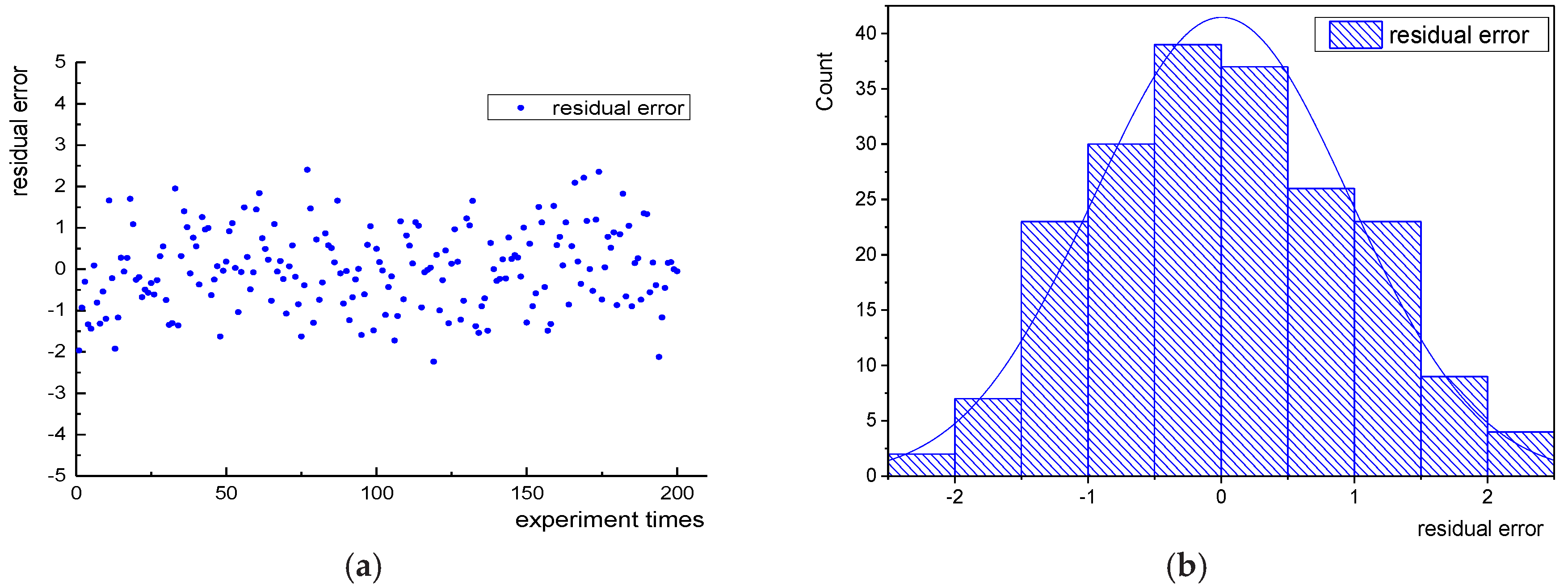
In order to verify the prediction accuracy of the hybrid DDTree model and the prediction ability of the model, the residual values of different models were obtained by calculating the prediction time and the actual value. The smaller the residual value, the stronger the prediction ability of the model, and the model fully learns the characteristics of the data from the training dataset. The residual analysis plots were created from the two models. Figure 11a,b shows the distribution plots of residuals and the residual histograms.

Figure 11. Residual analysis of the prediction results of the hybrid DDTree model: (a) the plot of residuals, (b) the residual histogram.

In Figure 11a, the waterway depth residual error value fluctuates around 0, which means that it is consistent with the actual prediction results and shows no bias. It can be seen from the results of two experiments that there are significant differences in the prediction of waterway depth results in the areas with small depths, such as near islands and shoal edges. The residual depth difference of this part is also significantly higher than other areas. In other deep-water navigation areas, the waterway depth predicted by the DDTree model is closer to the actual waterway depth, so the residual value of this part of the prediction of waterway depth result is smaller. In addition, in Figure 7 and Figure 9, there are also obvious differences at the edges of the navigation areas at different depths where the residual value is large. The waterway depth information of this part of the channel tends to fluctuate greatly, and it is affected by the hydrological and meteorological conditions. Therefore, the prediction results using the DDTree model can show a certain degree of error.

Figure 11b shows the sample distribution of the residual values. Most of the residual values are around 0. The residuals of the overall prediction of waterway depth are in accordance with the normal distribution, so the DDTree model can predict the waterway depth information of the waterway channel without bias.

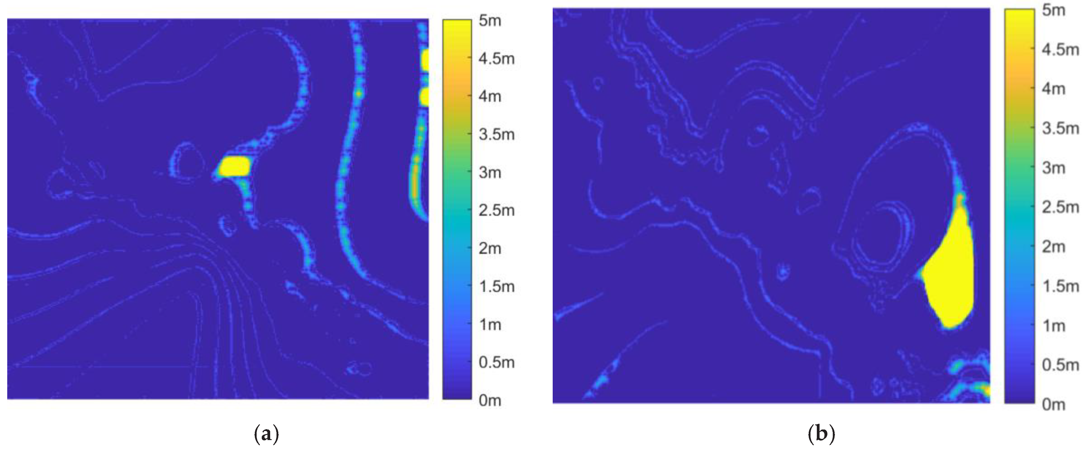
Figure 12 shows a difference plot between the ground truth depth map and predicted depth map for Nantong Port (Figure 12a) and Fangcheng Port (Figure 12b), respectively. One can note that the errors mostly concentrate on the boundaries of different seafloor depth zones. However, there are two areas with notable depth errors, which may be explained by the lack of AIS data in these areas.

Figure 12. Difference plot between the ground truth depth map and the predicted depth map for Nantong (a) and Fangcheng (b) ports.

We also compared and analyzed the traditional DNN model and decision tree model. Table 3 shows the prediction results of the model using different parameters. After the evaluation of the model, we chose the mean square error (MSE) as an indicator to calculate the deviation of the predicted value from the actual value, and reflect the prediction ability of the model. Table 3 shows a comparative analysis of the performance of the two models on the actual bathymetry data.

Table 3. Results of depth classification: mean square error (MSE) and coefficient of determination ($R^2$).

	Deep Neural Network	Hybrid DDTree Model
MSE	6.71	5.23
$R^2$	0.82	0.84
${\mathit{F}}_1$	0.61	0.85

In predictive analysis, the confusion matrix is a table composed of false positives, false negatives, true positives, and true negatives. The confusion matrix function evaluates accuracy by computing the confusion matrix with each row corresponding to the true class. In Equation (8), $\mathit{P}$ indicates the precision; R is the recall; and F is used to measure the value of precision and recall—it is the harmonic mean of precision and recall values. When $\mathit{\alpha }$ = 1, ${\mathit{F}}_{\mathbf{1}}$ score is calculated for performance evaluation.

$$F=\frac{\left(1+{\alpha }^2\right)PR}{{\alpha }^2\left(P+R\right)},$$

(8)

In Table 3, MSE and the coefficient of determination (${\mathit{R}}^2$) are used to demonstrate the performance of the model; MSE is used to measure the prediction error of the model and ${\mathit{R}}^{\mathbf{2}}$ is used to measure the accuracy of the prediction. We can see that the MSE value of the DDTree model is small and the ${\mathit{R}}^{\mathbf{2}}$ value is close to 1. Besides, the ${\mathit{F}}_{\mathbf{1}}$ score of the Hybrid DDTree model is 0.85 and the value of the deep neural network is 0.61, which means the hybrid DDTree model has better prediction performance. Thus, the waterway depth was predicted accurately using the hybrid DDTree Model. The hybrid DDTree model has a higher performance than the stand-alone DNN model.

5. Conclusions and Future Work

Depth of the waterway is a critical factor in the safety of marine traffic. However, due to the uncertainty of the waterway depth, it is difficult to obtain accurate waterway depth data in a timely manner. In this paper, we used the waterway depth data available from Global Mapper and the AIS data, together with the proposed DDTree model to predict the waterway depth data. The decision tree model is used to select the optimal attributes, and the AIS data are processed using the DNN. Then the neural network learns to perform inference reasoning on the sufficient waterway depth based on the ship’s behavior (the ship did not go aground). The experimental results show that the DDTree model has higher accuracy for prediction of waterway depth and can complete prediction of waterway depth more efficiently. Thus, it can compensate for the lack of waterway depth data in marine transportation and provide for faster update of waterway depth data. The results for prediction of depth using DDTree had an accuracy rate up to 91.15%.

However, there are still some disadvantages of prediction of waterway depth through DNN, as the network parameters can influence the prediction ability of DNNs. In future research, firstly, the sources of waterway depth data will be expanded, and the prediction methods will be optimized. Secondly, we hope to get inspiration from [41] to improve the resource utilization of our proposed model and enhance the security and data processing capacity of the prediction of waterway depth. Besides, DNNs and large-scale flow data processing will be considered to optimize network parameters, and a visual module will be introduced to display the map of predicted depth data in real time, which will improve the safety of marine transportation and will provide a reference for the smart navigation of ships.

References

1. UNCTAD. Review of Maritime Transport 2018. In Technical Report UNCTAD/RMT/2018; United Nations Conference on Trade and Development: New York, NY, USA, 2019. [Google Scholar]
2. Liu, C.; Mao, Q.; Chu, X.; Xie, S. An Improved A-Star Algorithm Considering Water Current, Traffic Separation and Berthing for Vessel Path Planning. Appl. Sci. 2019, 9, 1057. [Google Scholar] [CrossRef]
3. Briggs, M.J.; Silver, A.L.; Kopp, P.J. Probabilistic model for predicting ship underkeel clearance: Field and laboratory validation. Coast. Eng. J. 2014, 56, 3–822. [Google Scholar] [CrossRef]
4. Graziano, M.D.; Renga, A.; Moccia, A. Integration of Automatic Identification System (AIS) Data and Single-Channel Synthetic Aperture Radar (SAR) Images by SAR-Based Ship Velocity Estimation for Maritime Situational Awareness. Remote Sens. 2019, 11, 2196. [Google Scholar] [CrossRef]
5. Guo, D.; Yang, Y.; Xiong, F. Statistics and Analysis of Maritime Traffic Accidents in Yangtze River and Accidents Prediction. In Proceedings of the 28th International Ocean and Polar Engineering Conference, Sapporo, Japan, 10–15 June 2018. [Google Scholar]
6. Kamolov, A.; Park, S. An IoT-Based Ship Berthing Method Using a Set of Ultrasonic Sensors. Sensors 2019, 19, 5181. [Google Scholar] [CrossRef] [PubMed]
7. He, W.; Li, Z.; Malekian, R.; Liu, X.; Duan, Z. An Internet of Things Approach for Extracting Featured Data Using AIS Database: An Application Based on the Viewpoint of Connected Ships. Symmetry 2017, 9, 186. [Google Scholar] [CrossRef]
8. Al-Zaidi, R.; Woods, J.; Al-Khalidi, M.; Alheeti, K.M.A.; McDonald-Maier, K. Next generation marine data networks in an IoT environment. In Proceedings of the 2017 Second International Conference on Fog and Mobile Edge Computing (FMEC), Valencia, Spain, 8–11 May 2017; pp. 50–55. [Google Scholar] [CrossRef]
9. Venckauskas, A.; Stuikys, V.; Damasevicius, R.; Jusas, N. Modelling of internet of things units for estimating security-energy-performance relationships for quality of service and environment awareness. Secur. Commun. Netw. 2016, 9, 3324–3339. [Google Scholar] [CrossRef]
10. Capizzi, G.; Sciuto, G.L.; Woźniak, M.; Damaševičius, R. A clustering based system for automated oil spill detection by satellite remote sensing. In Proceedings of the 15th International Conference on Artificial Intelligence and Soft Computing, ICAISC 2016, Zakopane, Poland, 12–16 June 2016; pp. 613–623. [Google Scholar] [CrossRef]
11. Tu, E.; Zhang, G.; Rachmawati, L.; Rajabally, E.; Huang, G.-B. Exploiting AIS data for intelligent maritime navigation: A comprehensive survey from data to methodology. IEEE Trans. Intell. Transport. Syst. 2018, 19, 1559–1582. [Google Scholar] [CrossRef]
12. Su, H.; Liu, H.; Wu, Q. Prediction of Water Depth from Multispectral Satellite Imagery—The Regression Kriging Alternative. IEEE Geosci. Remote Sens. Lett. 2015, 12, 2511–2515. [Google Scholar]
13. Kang, C. A Differential Dynamic Positioning Algorithm Based on GPS/Beidou. Procedia Eng. 2016, 137, 590–598. [Google Scholar] [CrossRef]
14. Maciuk, K. Advantages of combined GNSS processing involving a limited number of visible satellites. Sci. J. Sil. Univ. Technol. 2018, 98. [Google Scholar] [CrossRef]
15. Chen, H. Travel-time approximation of acoustic ranging in GPS/Acoustic seafloor geodesy. Ocean Eng. 2018, 84, 133–144. [Google Scholar] [CrossRef]
16. EL-Hattab, A.I. Influence of GPS antenna phase center variation on precise positioning. NRIAG J. Astron. Geophys. 2013, 2, 272–277. [Google Scholar] [CrossRef]
17. Abdel-Hafez, M.F. On the GPS/IMU sensors’ noise estimation for enhanced navigation integrity, Mathematics and Computers in Simulation. Int. Assoc. Math. Comput. Simul. 2012, 86, 101–117. [Google Scholar] [CrossRef]
18. Younis, B.A.; Sousa, V.; Meireles, I. Prediction of the Asymptotic Water Depth in Rough Compound Channels. J. Irrig. Drain. Eng. 2009, 135, 231–234. [Google Scholar] [CrossRef]
19. Shiri, J. Wavelet and neuro-fuzzy conjunction model for predicting water table depth fluctuations. Hydrol. Res. 2012, 43, 286–300. [Google Scholar]
20. Wang, Y.; Zhang, J.; Chen, X.; Chu, X.; Yan, X. A spatial–temporal forensic analysis for inland–water ship collisions using AIS data. Saf. Sci. 2013, 57, 187–202. [Google Scholar] [CrossRef]
21. Vodas, M.; Pelekis, N.; Theodoridis, Y.; Ray, C.; Karkaletsis, V.; Petridis, S.; Miliou, A. Efficient AIS Data Processing for Environmentally Safe Shipping. Spoud. J. Econ. Bus. 2014, 63, 181–190. [Google Scholar]
22. Li, S.; Chen, X.; Chen, L.; Chen, L.; Zhao, Y.; Sheng, T.; Bai, Y. Data Reception Analysis of the AIS on board the TianTuo-3 Satellite. J. Navig. 2017, 70, 761–774. [Google Scholar] [CrossRef]
23. Mulyadi, Y.; Kobayashi, E.; Wakabayashi, N.; Pitana, T.; Wahyudi. Development of ship sinking frequency model over Subsea Pipeline for Madura Strait using AIS data. WMU J. Marit. Aff. 2014, 13, 43. [Google Scholar]
24. Li, J.; Chu, X.; He, W.; Ma, F.; Malekian, R.; Li, Z. A Generalised Bayesian Inference Method for Maritime Surveillance Using Historical Data. Symmetry 2019, 11, 188. [Google Scholar] [CrossRef]
25. Salmalian, K.; Soleimani, M. ANFIS and neural network for modeling and prediction of ship squat in shallow waters. Int. J. Math. Models Methods Appl. Sci. 2011, 5, 848–856. [Google Scholar]
26. Niu, H.; Ozanich, E.; Gerstoft, P. Ship localization in Santa Barbara channel using machine learning classifiers. J. Acoust. Soc. Am. 2017, 142, EL455–EL460. [Google Scholar] [CrossRef] [PubMed]
27. Bannari, A.; Kadhem, G. MBES-CARIS Data Validation for Bathymetric Mapping of Shallow Water in the Kingdom of Bahrain on the Arabian Gulf. Remote Sens. 2017, 9, 385. [Google Scholar] [CrossRef]
28. Kim, K.; Lee, K.M. Deep Learning-Based Caution Area Traffic Prediction with Automatic Identification System Sensor Data. Sensors 2018, 18, 3172. [Google Scholar] [CrossRef]
29. Jeong, M.; Lee, E.; Lee, M.; Jung, J. Multi-criteria route planning with risk contour map for smart navigation. Ocean Eng. 2019, 172, 72–85. [Google Scholar] [CrossRef]
30. Rong, H.; Teixeira, A.P.; Guedes Soares, C. Data mining approach to shipping route characterization and anomaly detection based on AIS data. Ocean Eng. 2020, 198. [Google Scholar] [CrossRef]
31. Xin, X.; Liu, K.; Yang, X.; Yuan, Z.; Zhang, J. A simulation model for ship navigation in the “Xiazhimen” waterway based on statistical analysis of AIS data. Ocean Eng. 2019, 180, 279–289. [Google Scholar] [CrossRef]
32. Zhang, L.; Meng, Q.; Fwa, T.F. Big AIS data based spatial-temporal analyses of ship traffic in singapore port waters. Transp. Res. Part E Logist. Transp. Rev. 2019, 129, 287–304. [Google Scholar] [CrossRef]
33. Yang, D.; Wu, L.; Wang, S.; Jia, H.; Li, K.X. How big data enriches maritime research–a critical review of automatic identification system (AIS) data applications. Transport. Rev. 2019, 39, 755–773. [Google Scholar] [CrossRef]
34. D’Angelo, G.; Tipaldi, M.; Glielmo, L.; Rampone, S. Spacecraft autonomy modeled via Markov decision process and associative rule-based machine learning. In Proceedings of the 2017 IEEE International Workshop on Metrology for AeroSpace (MetroAeroSpace), Padua, Italy, 21–23 June 2017; pp. 324–329. [Google Scholar] [CrossRef]
35. D’Angelo, G.; Pilla, R.; Tascini, C.; Rampone, S. A proposal for distinguishing between bacterial and viral meningitis using genetic programming and decision trees. Soft Comput. 2019, 23, 11775–11791. [Google Scholar] [CrossRef]
36. Lee, E.; Mokashi, A.J.; Moon, S.Y.; Kim, G. The Maturity of Automatic Identification Systems (AIS) and Its Implications for Innovation. J. Mar. Sci. Eng. 2019, 7, 287. [Google Scholar] [CrossRef]
37. Woźniak, M.; Połap, D. Hybrid neuro-heuristic methodology for simulation and control of dynamic systems over time interval. Neural Netw. 2017, 93, 45–56. [Google Scholar] [CrossRef] [PubMed]
38. Połap, D.; Woźniak, M.; Damaševičius, R.; Maskeliūnas, R. Bio-inspired voice evaluation mechanism. Appl. Soft Comput. J. 2019, 80, 342–357. [Google Scholar] [CrossRef]
39. Cagnini, H.E.L.; Barros, R.C.; Basgalupp, M.P. Estimation of distribution algorithms for decision tree induction. In Proceedings of the 2017 IEEE Congress on Evolutionary Computation, San Sebastian, Spain, 5–8 June 2017; pp. 2022–2029. [Google Scholar]
40. Bottou, L. Large-scale machine learning with stochastic gradient descent. In Proceedings of the 19th International Conference on Computational Statistics COMPSTAT, Paris, France, 22–27 August 2010; pp. 177–186. [Google Scholar] [CrossRef]
41. Połap, D.; Woźniak, M.; Wei, W.; Damaševičius, R. Multi-threaded learning control mechanism for neural networks. Future Gener. Comput. Syst. 2018, 87, 16–34. [Google Scholar] [CrossRef]
Article Metrics
Citations
Article Access Statistics
Multiple requests from the same IP address are counted as one view.