Article

Prediction of High Capabilities in the Development of Kindergarten Children

1
Centro de Innovación y Desarrollo Tecnológico en Cómputo, Instituto Politécnico Nacional, Ciudad de México 07700, Mexico
2
Center for Pedagogical Studies and Department of Computer Sciences of the University of Ciego de Ávila, Ciego de Ávila 67100, Cuba
3
Centro de Investigación en Computación, Instituto Politécnico Nacional, Ciudad de México 07700, Mexico
*
Author to whom correspondence should be addressed.
Appl. Sci. 2020, 10(8), 2710; https://doi.org/10.3390/app10082710
Submission received: 24 March 2020 / Revised: 2 April 2020 / Accepted: 2 April 2020 / Published: 14 April 2020

Abstract

:
Analysis and prediction of children’s behavior in kindergarten is a current need of the Cuban educational system. Despite such an early age, the kindergarten institutions are devoted to facilitate the integral children development. However, the early detection of high capabilities in a child is not always accomplished accurately; due to teachers being mostly focused on the performance of the children that are lagging behind to achieve their age range’s stated goals. In addition, the amount of children with high capabilities is usually low, which makes the prediction an imbalanced data problem. Thus, such children tend to be misguided and overlaid, with a negative impact in their sociological development. The purpose of this research is to propose an efficient algorithm that enhances the prediction in the kindergarten children data. We obtain a useful set of instances and features, thus improving the Nearest Neighbor accuracy according to the Area under the Receiving Operating Characteristic curve measure. The obtained results are of great interest for Cuban educational system, regarding the rapidly and precise prediction of the presence or absence of high capabilities for integral personality development in kindergarten children.

1. Introduction

The goal for children in the earliest stages of childhood in Cuba is to achieve the maximum possible integral development in each child. This goal imposes a challenge regarding the attention to the diverse kinds of children within the Cuban children’s institutions belonging to the Ministry of Education. To this end there is a marked interest in detecting children that possess high development potential, since seldom do these children receive an education that is tailored to their potential.
Children with high development potential need specific learning strategies so that their development can be enhanced [1,2,3]. Cuban pedagogy wagers on teaching styles that respect individual differences and grant each child the ability to assimilate knowledge at his or her own pace, in a personalized way and according to each individual’s needs. In this sense, several advances have been made in Cuba regarding attention to children with learning difficulties as well as those with special needs such as blind, deaf and motor-impaired children. However, attention to kindergarten children with high development potential has not received the same amount of attention, neither theoretical nor practical, in Cuba.
Among the causes of this phenomenon is the fact that high-capabilities children do not represent a threat for the performance scores of educational institutions. This results in teachers focusing on helping the children that are lagging behind to achieve their age range’s stated goals; leaving high-capabilities children without specialized attention.
In addition, the theoretical foundation of high capabilities in the early stages of childhood has not been fully developed. Most research aimed at superior potential detection focuses on children over five years old [4,5], leaving a void in researching detection at an early age [6]. High capabilities can show up in fields so apart from each other, such as music and mathematics, which makes it a complex phenomenon that is hard to define and identify [7]. Even though psychological studies have been carried out to detect it, most of them involves the use of complex tests that need to be interpreted by highly-qualified personnel [6].
The absence of easily measurable indicators turns early detection of children with high capabilities into a nearly impossible task for the personnel in charge of preschool education in Cuba. This results in an affectation to the differentiated attention process that such children need, since their detection and further access to pedagogical attention is compromised. In several occasions, this lesser pedagogical stimulation results in the children not reaching their full intellectual potential and underachieving [2,8,9]. Additionally, the lack of differentiated attention results in a lessened social development in these children, who can end up isolated from their peers and therefore lacking the expected social skills for their age [10,11].
We want to emphasize that, in Cuba, that the strategies for the pedagogical management of children with high-potential exist, and are detailed in the methodological procedures of the education system. However, they are useless if the educational personnel in charge do not detect the children with high-potential, that is, if they do not detect the child, they do not apply what is established, and the development of the child is affected.
It is for these reasons that the Center for Pedagogical Studies of the University of Ciego de Ávila is undertaking field research aimed at improving pedagogical attention for high-potential children, which are classified as having special educational needs according to the Cuban educational system. This study aims to use easily measurable and understandable indicators along with advanced pattern recognition and data mining techniques as tools to determine the characteristics of gifted children. Thus, these children would be identified earlier and the design and application of pedagogical strategies tailored to them would become easier. In this way, the expectation is to achieve the best possible development for each child.
One of the requirements of computer-aided prediction in educational environments is the decision explanation capability of the used model. The Nearest Neighbor (NN) classifier [12] is one of the simplest yet accurate algorithms for non-parametric prediction, and its ability of returning the neighbors of an unclassified pattern makes it very suitable for soft sciences prediction problems. The NN classifier had been used previously to successfully solve educational problems in Cuba, such as family classification [13].
However, the NN classifier heavily depends on the dissimilarity function used. To detect children with high capabilities, the design of a specific dissimilarity function is needed, in order to successfully compare the children descriptions. To address this issue, the present paper includes the design of a specific dissimilarity function for the NN classifier in the detection of children with high capabilities for the integral personality development.
NN classifier is also sensitive to noisy features and mislabeled or outlier training instances, but these drawbacks may be overcome by the elimination of irrelevant features and instances. To preprocess the kindergarten children data, we propose a novel algorithm that selects both relevant features and instances. Our proposal integrates some elements of the Rough Set Theory [14] and a structuration strategy of logical-combinatorial pattern recognition [15].

2. Materials and Methods

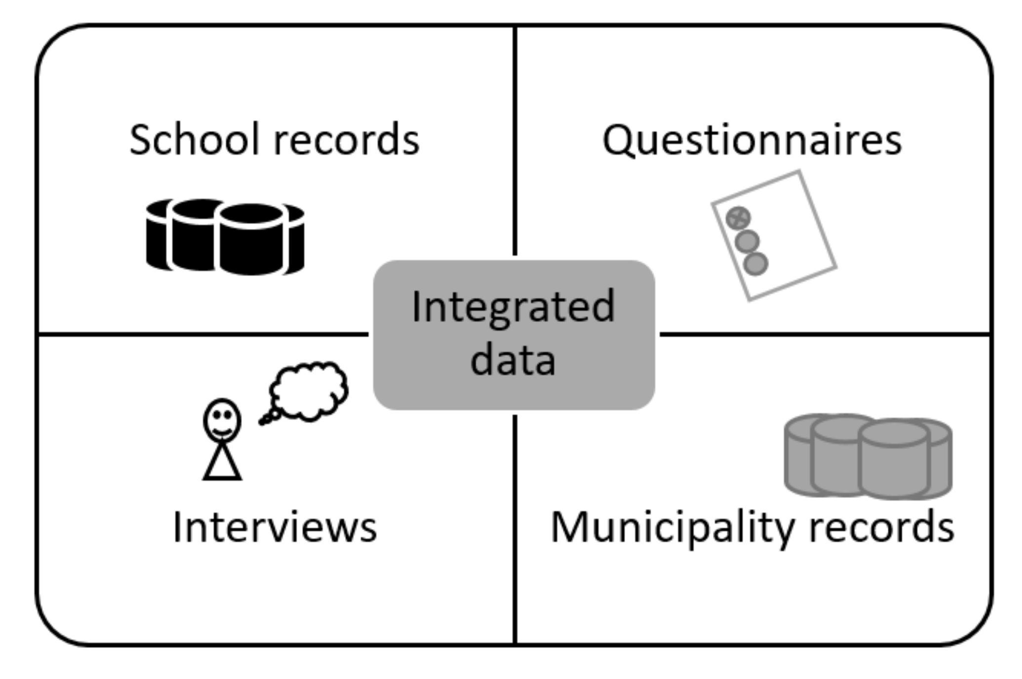
2.1. The Kindergarten Children Data

The Cuban children of five years of age carried out their studies on the kindergarten facilities of the Cuban educational system. All of them are government facilities. The Cuban educational system is under two ministries: the Ministry of Education, and the Ministry of Superior Education. The last one is just for university and postgraduate education, while the former includes all other forms of education. The Ministry of Education includes special facilities for children with social and behavioral maladies (SBAM), as well as special facilities for children with disabilities (blind, deaf, motor problems, mental retardation, among others). Most of the educational population is under regular facilities, divided into four stages: nursery school (1–5 years old), elementary (6–11 years old), secondary (12–14 years old) and high school (15–17 years old, non-mandatory). Our research is focused on children of the preschool year, that is, children of five years old. Such children can be in classrooms at nursery school facilities or in classrooms at elementary school facilities. It is important to mention that the preschool year is the first mandatory school year in Cuba. Therefore, all children must be in the corresponding classroom.
The study of which features potentially intervene in the presence of high capabilities for development in children was the first step in this research. For this purpose, pedagogical and sociological research was taken into account [3,4,5,8,16], as well as the professional experience of teaching personnel at the preschool level. In addition, other situations that may influence detection such as environmental and socioeconomic factors were analyzed [2].
The process for data integration considered several sources of data: Data stored in school records (related to children performance and behavior), data collected from questionnaires and interviews to families (related to lifestyle, antecedents and others) and data stored in municipality records (related to environmental and socioeconomic factors). We want to emphasize that all such data were collected with the consent of the parents and the corresponding authorities. In addition, all surveys and questionnaires were carried out by qualified personnel, and all the instruments used had the corresponding validation. Figure 1 shows the data integration process.
The collected features are divided into five groups. The first one is related to the child and its antecedents. The features considered in this group were the child’s age, its gender, whether its family supports its development (family), whether someone in the family has a history of high potential (antecedents), whether the child received schooling prior to entering preschool (prior education) and the performance of the teaching agent in charge of the child (performance).
The second group of features alludes to the attributes of the child’s environment. These are the nutritional status of the child (nutrition), the hygiene level of the household (hygiene), the presence of healthy lifestyles at home (lifestyle), the structural conditions of the dwelling (dwelling) and the characteristics of the home’s neighborhood (environment, considered as favorable, average or socially challenging).
The third attribute group evaluates the product of the child’s activity within its educational institution. For this purpose, the situations considered were the quality of the child’s schoolwork (quality), the quickness with which the child solved the required tasks (speed), the originality of the child’s proposed solutions (originality) and the tendency to help other children with their tasks in addition to their own (help).
The fourth group of attributes focuses on characterizing the child’s relationship with their educational environment. In this sense, the features analyzed are the level of interest and participation of the child in collective playtime (play), the child’s tendency to interact with other children or to remain alone (relationships), whether the child prefers the company of an adult to that of other children (adult) and whether the child is active and energetic (activity).
The fifth feature group takes into account subjective aspects related to the perception that the child has of itself and of its environment. In this group are included: whether the child shows a heightened curiosity about its surroundings (curiosity), whether it shows a high level of interest in its environment (interest), whether the child becomes easily bored with simple tasks (boredom), whether the child feels superior to its peers (superiority) and its self-esteem level (self-esteem, measured as low or high). In all, 24 potential attributes were considered and are shown in Table 1.
Taking into account the attributes that are potentially influential in the characterization of high-capabilities Cuban preschool children, a data collection process was undertaken.
For this purpose, these features were evaluated in children from five preschool classrooms in the municipality of Ciego de Ávila, Cuba, in the school years 2014–2018. The teaching personnel was in charge of the description of its own students, except for attribute #6, performance, which was input by the administrative staff in charge of the teachers, according to the performance evaluation of each worker. In total, we obtained the description of 1032 children. Of them, 91 were marked as having high-potential, for an imbalance ratio of 11.34.
It is important to mention that during the data collection process, not every attribute was able to be obtained for every student; in the majority of cases, this was because the teacher was unable to find the right information or was unsure about its accuracy. This resulted in the presence of missing values in the description of the children.

2.2. Data Mining Algorithms

In order to perform automated detection of high-capabilities children, data mining and pattern recognition techniques were employed. It is known that not every pattern classifier is able to explain its inner workings [17]. It is for this reason that for this research it was decided to use a classifier (Nearest Neighbor, NN) [12] that is able to explain how it arrived at a determined prediction.
NN was proposed by Cover and Hart back in 1967. It stores a set of training instances, and when a new instance arrives, it computes its distance (or dissimilarity) with respect to every instance in the training set. Then, it classifies the novel instance with the class of its closest (nearest) instance.
In addition, the presence of missing values represents a challenge for most classification algorithms [18], which complicates their application to problems presenting this kind of data. Along with this, most classifiers assume the presence of either numerical or categorical attributes, and are not prepared to deal with mixed data. In the problem of detecting high-capabilities Cuban preschoolers we have 23 categorical features, one numerical feature (age) and several incomplete descriptions. This makes the application of some pattern classifiers difficult.
To apply the Nearest Neighbor classifier to the data we need to define, with the support of educational specialists, a dissimilarity function to compare children descriptions. The designed function is non-symmetric, given that the feature comparison criterion of feature “house” is non-symmetric. Having two children description n i and n j the dissimilarity function to compare them is given as:
d n i , n j = k = 1 l d k n i , n j
where l denotes the amount of features, and d k is the feature comparison criterion for the k-th feature.
For the numeric attribute “age”, we used normalized difference as comparison criterion, as in Equation (2). m a x k and m i n k denote the maximum and minimum values of the k-th feature.
d k n i , n j =   n i k n j k m a x k m i n k
Additionally, we used classical comparison criteria, as in Equation (3) for the categorical features with two admissible values (features 2, 3, 4, 5, 7, 10–13 and 16–24). For the other features, we used the comparison criterion defined in the corresponding table.
d k n i , n j = 1   i f   n i k n j k 0   i f   n i k = n j k  
To handle missing values (denoted by “?”), we decided to set the dissimilarity value d k n i , n j = 0.5 if n i k = ? n j k = ? , as numeric and categorical comparison criteria are defined between the [0,1] interval. For the feature “speed”, we use the feature values dissimilarity matrix showed in Table 2 as comparison criterion.
In addition, features “quality”, “performance”, “environment” and “house” have comparison criteria showed in Table 3, Table 4, Table 5 and Table 6, respectively.
The similarities among feature values for the attributes “environment” and “house” were determined according to the criteria of specialist of the Municipal Investment Unit of Dwelling (UMIV), in Ciego de Avila, Cuba.
As mentioned earlier, the Nearest Neighbor classifier is sensitive to noisy or mislabeled instances, as well as to irrelevant attributes. To overcome these drawbacks, we propose a novel algorithm for selecting both useful cases and features. The proposed algorithm is described in the next section.

3. Data Preprocessing

The proposed algorithm is based on Rough Set Theory (RST), and it is inspired in some elements of selecting pools of classifiers. The next section is devoted to the explanation of some basic RST concepts.

3.1. Fundamentals of Rough Set Theory

Pawlak introduced Rough Set Theory in 1982 [14] to deal with vague and imprecise information. Since then, it have been successfully applied to data preprocessing in both cases and attributes selection [19]. Let A be a set of features and a non-empty set U (universe) of instances described by the features in A; the pair (U,A) is denoted as the information system. If every element of U has also an additional decision feature c, then it is obtained a decision system, D S ( U , A c ), where c A [14].
Classical (often called Pawlak’s) RST considers that a feature A i A distinguishes an instance x from another instance y, and it is denoted by D i s t i n g u i s h e s ( A i , x , y ) , if and only if all their feature vales are different; that is, D i s t i n g u i s h e s ( A i , x , y ) x i y i ,   A i A .
Every subset of features B of A has associated a binary inseparability relation I N D B U , which is formed by the set of pairs of instances indistinguishable by the relation; that is, the instances having the same feature values in the set of features B. Formally, I N D B U = x , y U × U : ~ D i s t i n g u i s h e s B i , x , y ,     B i B . An inseparability or indiscernibility relation defined by forming subsets of elements from U having the same feature values for a subset of features B A , is an equivalence relation.
The indistinguishable instances form an equivalence class. The equivalence class of an instance x with respect to the indiscernibility relation induced by the features in B, is denoted by x B .
RST incorporates a very interesting concept, the reduct definition. A reduct is a set of features BA such that I N D B X = I N D A X ; that is, both B and A generate the same partition of the universe U. In Pawlak’s words “a reduct is the minimal set of attributes that enables the same classification of elements of the universe as the whole set of attributes. In other words, attributes that do not belong to a reduct are superfluous with regard to classification of elements of the universe” [14].
Following these considerations, the computation of the set of reducts in a dataset is a kind of feature selection (by deleting those features, which do not belong to the obtained reducts), and have been extensively used [20]. In this research, we include the computation of all reducts to perform feature selection the proposed algorithm.
RST also considers that every concept can be roughly approximated. Let it be a decision system DS = U , A c and let it be the sets B and X such that BA and XU. The concept X can be roughly approximated using the information contained in B by constructing the B-inferior (B-lower) and B-superior (B-upper) approximations, denoted by I N F B X and S U P B X , respectively; and defined as follows: I N F B X = x U : x B X and S U P B X = x U : x B X . The instances in I N F B X are with certainty members of X while the instances in S U P B X are possible members of X. The limit region for the concept X is computed as L I M B X = S U P B X I N F B X .
The information in the lower and upper approximations of a rough set have been used for the task of selecting relevant instances [21]. In this paper, we also used that information. However, we use Minimum Neighborhood Rough Sets (MNRS) [21] instead of Pawlak’s.

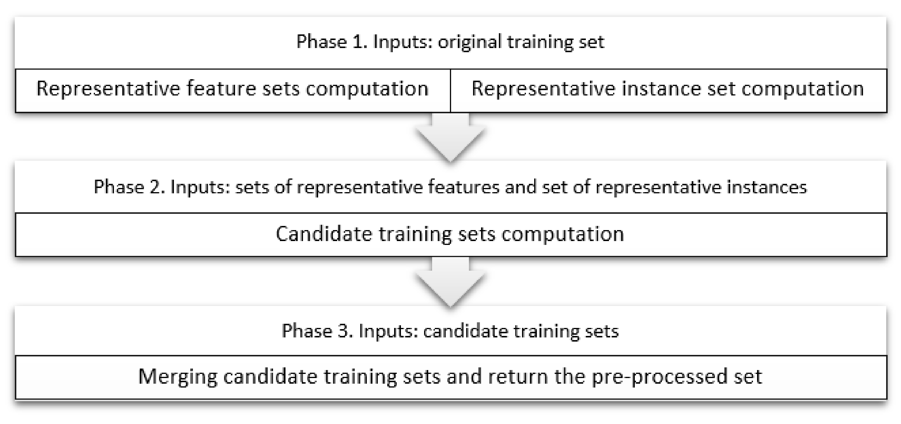
3.2. Proposed Preprocessing Technique

The proposed algorithm consists of three phases. The first phase consists of the parallel selection of relevant features and relevant instances of the training set. Then, the second phase obtains a candidate training sets, composed by the selected features and instances. Finally, the candidate training sets are merged in the third phase of the algorithm. As the main highlights of the algorithm, we consider its ability to handle mixed and incomplete datasets, with class imbalance. The three phases of the proposed algorithm, named FIS-SM (Feature and Instance Selection, with Sigmoid Merging) are described in detail in the next subsections.

3.2.1. Parallel Computation of Relevant Features and Instances

The algorithm starts by executing two separated processes over the training set: selection of relevant feature sets, and selection of relevant instances (Figure 2). The selection of relevant feature sets consist on the computation of all reducts of the training sets, using the LEX algorithm [22].
On the other hand, to remove irrelevant instances, we decide to preserve decision boundaries, to keep as much as possible the minority class examples. We introduce a condensation algorithm, based on Minimum Neighborhood Rough Sets (MNRS) [21]. We selected MNRS due to its ability of handling missing and incomplete decision systems, and non-symmetric similarity functions. Those characteristics make MNRS very suitable to solving the preprocessing of the Cuban kindergarten data.
In a Minimum Neighborhood Rough Set, the positive and limit regions of the decision classes are computed according to the relations between instances in a Maximum Similarity Graph (MSG). A MSG is a directed graph such that each instance is connected with its most similar instance. Formally, two instances x and y belonging to the set X, for an arc in a MSG if and only if s i m x . y = m a x s i m x , z   z X where s i m , is a similarity function. The connected components of such graphs are named compact sets. Let θ be the arcs in a MSG, the lower approximation of a decision class Y i with respect to the feature set A, is defined as:
I N F A Y i = x Y i :   x , y θ ,   y Y i
The limit region of a decision class Y i is is given by the following:
L I M A Y i = x Y i :   x , y θ ,   y Y i
The algorithm proposed for selecting relevant instances consist on computing the limit region of each decision class, and using compact sets [15] to structure each class. Compact sets are the connected components of a Maximum Similarity Graph, and they have been used for instance selection, with very good results [23].
Let be U a universe of instances and a similarity function sim x , y where x , y U . A subset cs from U is a compact set if and only if:
(a)
x j U x i c s max x k U x k x i s i m x i , x k = s i m x i , x j max x k U x k x i s i m x k , x i = s i m x j , x i x j c s
(b)
x i , x j c s , x i 1 , , x i q c s x i = x i 1 x j   = x i q p   1 , , q 1 max x t U x t x i p s i m x i p , x t = s i m x i p , x i p + 1 max x t U x t x i p s i m x i p + 1 , x t = s i m x i p + 1 , x i p
(c)
Every isolated instance is a degenerated compact set.
After computed the compact sets, for each of them the algorithm finds a representative prototype, which is added to the prototype set, along with the instances in the limit region. This guarantees the preservation of the decision boundaries, as well as the inner representation of the class structure. The representative prototypes are computed as the instances that maximize the average similarity with respect to all instances in the compact set.
The pseudo code of the main steps for the proposed instance selection algorithm is presented as follows in Algorithm 1.
Algorithm 1. Pseudocode of the proposed algorithm.
Algorithm to compute the representative instance set
Inputs: training set X
Output: representative set C
Steps:
  • C =
  •  For each decision class Y i
    • C = C L I M Y i (as in Equation (5))
    •    Structure Y i in compact sets.
    •    For each compact set CS
    • C = C r where r = arg max x C S y C S s i m x , y C S
  • Return C
The obtained representative instance set along with the set of all reducts is given as inputs to the second phase of the proposed algorithms.

3.2.2. Computation of Candidate Training Sets

The second phase of the algorithm begins with the representation of the selected instances using only the features in the minimal reducts sets. That is, every minimal reduct will be used as the feature set to represent the selected instances (Figure 3) obtaining as many candidate training sets as minimal reducts computed.
Then, each candidate training set is postprocessed, by the application of the CSE algorithm [23] for further instance selection (Figure 4). Our proposal uses the CSE algorithm for additional instance selection because CSE is able to handle mixed and incomplete data descriptions, and preserves the inner structure of classes, due to it has the property of been subclass consistent [23].

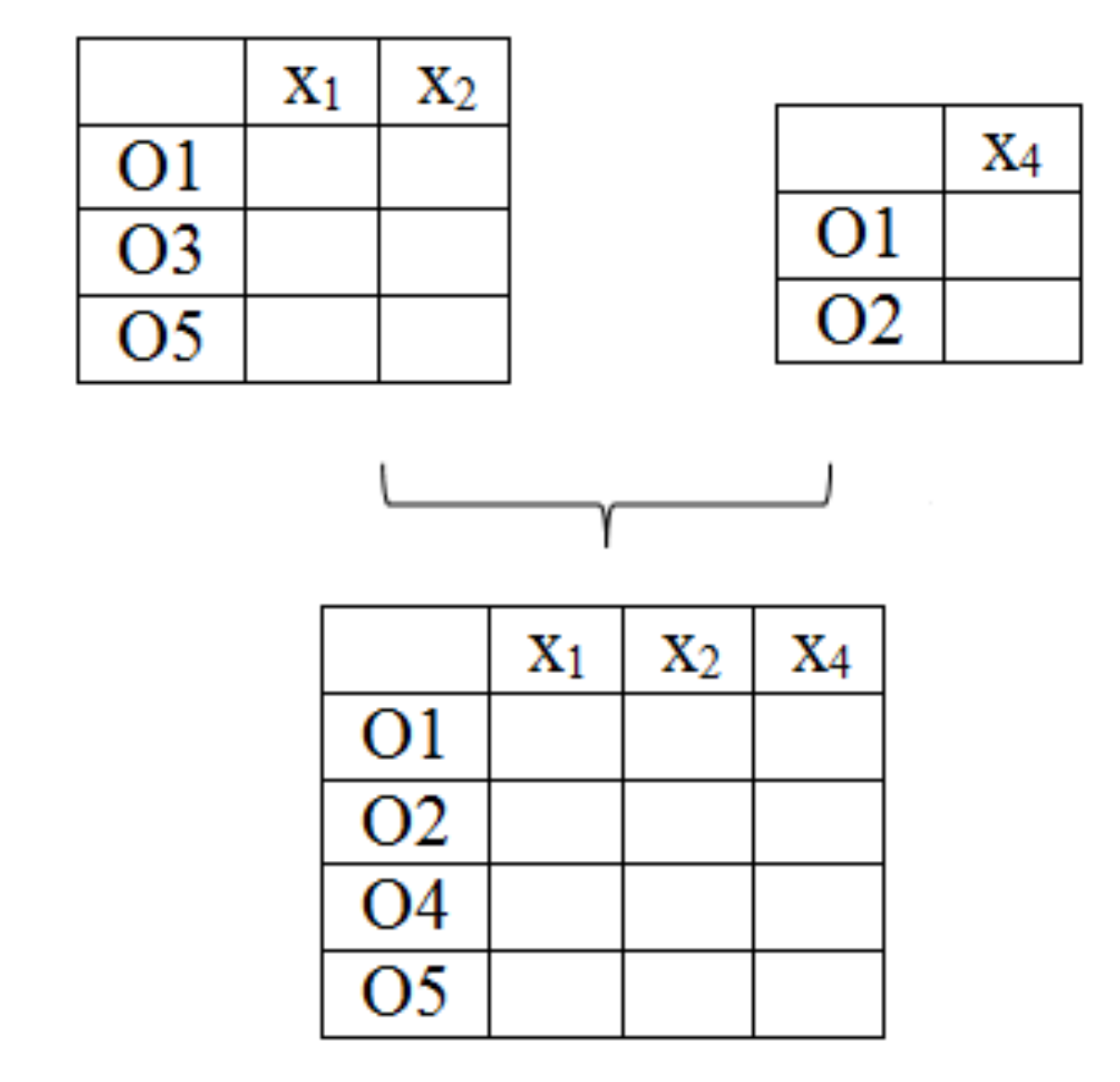
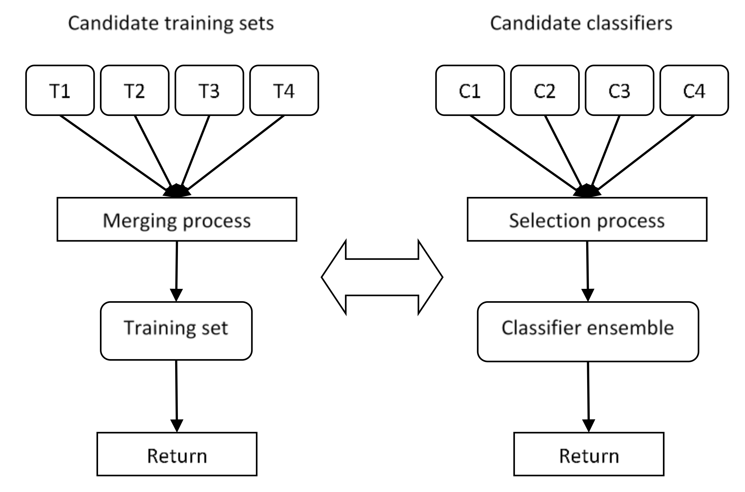
3.2.3. Merging of Candidate Training Sets

Although the application of extra instance selection in the second phase of the algorithm may cause some information loss, the merging phase compensates it. When two candidate training sets are merged, the resulting set contains the instances and features of both parent sets (Figure 5).
We viewed the merging process of candidate training sets as an equivalent of the selection of classifiers to form a classifier ensemble. In classifier selection to form ensembles, there is a pool of candidate classifiers, and they must be combined to form an ensemble [24]. In the merging process, there is a pool of candidate training sets, and they must be merged to form the final training set (Figure 6).
To carry out the merging phase, we introduced a novel procedure (Algorithm 2), inspired in the SA algorithm [25] to select a classifier ensemble form a pool of classifiers. SA uses classifier correlation and diversity to guide the selection.
Algorithm 2. Pseudocode of the proposed merging strategy.
Merging of candidate training sets
Inputs: Φ: correlation measure, T: set of candidate training sets, O: original training set
Output: preprocessed training set t b e s t
Steps:
  • Consider t b e s t T as the candidate training set with higher consistency factor (Equation (7)) and best as the associated consistency factor value.
  • possible = true
  • Select the candidate training set t T less correlated with tbest, as L = argmin t T Φ t b e s t , t
  • While ( b e s t < γ L t b e s t ) and (possible)
    •     t b e s t = L t b e s t
    •    Select the most accurate candidate training set to merge with the current tbest,
    •       S = argmax t T S i g t b e s t t , where S i g t b e s t t = 1 O o O s i g m o i d ρ .
    •    If γ t b e s t S > γ t b e s t then t b e s t t b e s t L
    •    else possible = false
  • Return t b e s t
We considered the RST measure consistency factor [14] as a degree of performance of the candidate training sets. The consistency factor ( γ ) considers the amount of instances in the lower approximation of concepts, with respect to the total amount of instances. Thus, the graters γ , greater amount of instances certainly belong to their classes.
Let us considered a set of instances X described by a set of features A, and a decision attribute c. The partition of the set X according to the decision attribute form the set Y = Y 1 , , Y k . The lower approximation of the corresponding decision system D S X , A c is given by:
I N F A Y = Y i Y I N F A Y i
Then, the consistency factor of the decision system is defined as:
γ A , Y = I N F A Y X
Taking into consideration the values of the consistency factor, we considered the candidate training set with higher γ as the current best, tbest.
Then, the procedure selects the less correlated candidate training set, with respect to tbest. If the merging of both sets outperforms the γ of tbest, tbest is replaced by the resultant training set, and an iterative process is carried out until no improvements are achieved. Otherwise, tbest is returned as the final preprocessed training set.
We used the sigmoid function as well as in [25] to potentiate the correct classification of as much instances as possible. For this task, we computed the Nearest Neighbor classification of the instances in the original (unprocessed) training set and we followed a procedure based on the sigmoid function. If both candidate training sets correctly classifies a case belonging to the original training set, then ρ = 5 . On the contrary, if both of them give an incorrect classification, ρ = 5 . Finally, if only one correctly classifies the case, ρ = 0 .
We used the Q measure recommended in [26] as a training set correlation measure. The Q measure has as advantages that it is independent of the amount of sets to considered, and obtained a zero value for independent training sets. By considered the correlation of the candidate training sets, the proposed merging strategy avoided fusions with no direct impact on the classifier accuracy.

4. Results and Discussion

In this section, we investigated the performance of the proposed FIS-SM algorithm for data preprocessing. We carried out two different numerical experiments. The first addressed the suitability of FIS-SM in selecting relevant instances and feature to solve the classification of Cuban kindergarten children with high capabilities. The second experiment evaluates the performance of the proposal over international datasets.

4.1. Results for Educational Data

As we were dealing with an imbalanced dataset, with imbalance ratio IR = 8.1, we used as a classifier performance measure the Area under the ROC curve (AUC). AUC is a performance measure that takes into consideration the amount of correctly classified instances of positive and negative classes [27]. This characteristic makes AUC suitable for the evaluation of classifier performance in imbalanced datasets, due to its lack of bias in favor of the majority class.
The AUC is based on the computation of two measures: the True Positive Rate (recall or sensitivity) and the True Negative Rate (specificity).
Let us consider the confusion matrix of Table 7. The True Positive Rate (TPR) and True Negative Rate (TNR) are computed as follows:
T P R = t p t p + f n
T N R = t n t n + f p
Accordingly, the Area under the ROC curve for a discrete classifier is computed as:
A U C = T P R + T N R 2
In addition to classifier performance, we computed the instance reduction rate and feature reduction rate. As the Nearest Neighbor classifier stores the training set in memory, and also compares the new instances to be classified with the ones stored in the training set, both instance and feature reduction measures indicate the amount of computational cost saved with the preprocessing algorithm.
We compared FIS-SM with respect to previously reported algorithms. Several genetic based algorithms were selected [28], such as the Genetic Algorithm proposed by Ishibushi and Nakashima (IN-GA) [29], the Genetic Algorithm proposed by Kuncheva and Jain (KJ-GA) [30] and the Genetic Algorithm proponed by Ahn, Kim and Han (AKH-GA) [31]. The hybrid Evolutionary Instance Selection enhanced by Rough set based Feature Selection (EIS-RFS) algorithm [19] was also selected for comparison. In addition, the deterministic algorithm for instance and feature selection proposed by Villuendas-Rey et al., the Testors and Compact set based Combined Selection (TCCS) [32] were considered in the comparison.
We also computed the results of the NN classifier without any preprocessing (ONN). The parameters for the compared algorithms are shown in Table 8. We used the corresponding papers for such parameter configuration.
In Table 9 we show the results of the compared algorithms over the kindergarten dataset. We highlight in bold the best results.
The results show that the proposed FIS-SM increased the classifier performance according to the AUC measure, using fewer instances and features. FIS-SM obtained an AUC very close to the perfect classification, with less than 7% of instances and with almost 27% of features. Having a reduced set of instances and features decreased the computational cost of the Nearest Neighbor classifier, and reduced the execution time. Let n be the number of instances and m the number of features in the training set. The classification cost of NN classifier was bounded by   O n × m , due to each instance to be classified need to be compared using a similarity function with an average cost of O m , with respect to every instance in the training set. Considering the results of the proposed FIS-SM, the cost after preprocessing will be O 0.93 × n × 0.73 × m .
In addition, the FIS-SM algorithm outperformed all compared algorithms according to AUC, instance reduction and feature reduction. The above results show the high quality of the proposed algorithm, and its ability to obtain a useful set of both cases and features in mixed, incomplete and imbalanced scenarios.
Considering the experiments carried out, we selected as relevant the features that were included in at least one fold. Therefore, our research points out that features 4, 13, 18, 19, 20, 21, 22 and 24 (antecedents, help, adult, play, curiosity, interest, boredom and superiority) are relevant to determine if a child has or has not high-potential for development.
Having an accurate automatic classification of kindergarten children allows the educational personnel to improve the pedagogical attention for high-potential children. The automatic classification alerts the personnel of the presence of gifted children, and the design and application of pedagogical strategies tailored to them would become easier. In addition, we see that the number of high-potential children in a classroom is usually very low. In the data collected from 2014 to 2018, the classroom having the greater number of such children only have four of them. Therefore, guaranteeing an automatic classification with high AUC (as the 0.95 obtained by our proposal) is a significant result, and a major aid to educational personnel in charge of the children.

4.2. Results for Repository Data

In addition to the excellent results obtained over the Cuban kindergarten dataset, we also consider that it was necessary to test the performance of the proposed algorithm over well-known repository datasets. To accomplish this task, we selected eight datasets from the UCI Machine Learning repository [33]. Table 10 gives the description of them. The IR column represents the imbalance ratio of the dataset, computed as the ratio between the instances in the majority and minority classes.
To consider the imbalanced class scenario, we included five datasets having I R > 1.5 . We also considered among the selected datasets seven having mixed numerical and categorical features, and five incomplete datasets.
To apply the NN classifier over the repository data, we selected as the dissimilarity function the HEOM dissimilarity [34]. We used the five-fold cross validation procedure and averaged the results. We selected five-fold cross validation due to its suitability for handling the imbalanced nature of some of the datasets [35].
As in the previous experiment, we computed the instance reduction ratio and the feature reduction ratio for the Nearest Neighbor classifier. However, to compare the classifier performance we could not use the Area under the ROC curve measure.
As the AUC is only applicable for a two class problems and we were dealing with several multiclass imbalanced data problems, and it is well known that classifier accuracy is biased to favor the majority class, we considered the computation of the average accuracy by classes (Avg_Acc) as a classifier performance measure [36].
Let be Y = Y 1 ,   ,   Y l the set of classes the averaged accuracy by classes is computed by:
A v g _ A c c = 1 Y Y i Y 1 Y i x Y i w e l l x w e l l x = 1 if   x   is   correctly   classified 0 otherwise
We considered that the computation of the average accuracy by classes eliminates the bias of the traditional classifier accuracy and allows us to compare the classifier performance over multiclass imbalanced datasets. This computation is also provided in the summary results of the Explorer module of the Weka software [37].
Table 11 offers the Avg_Acc results of the Nearest Neighbor classifier without preprocessing (ONN), as well as the results of TCCS, EIS-RFS and the proposed FIS-SM. Best results are highlighted in bold.
The averaged accuracy results over the repository datasets favored the proposed FIS-SM, which obtained the best classifier performance in four datasets. We considered that this behavior was due to FIS-SM being designed to deal with imbalanced data, a key feature that allows it to maintain good classifications in the datasets.
However, according to the instance retention rate (Table 12) the EIS-RFS algorithm was the best. In all datasets it achieved the best instance reduction rates, with over 93% reduction. On the other hand, the proposed FIS-SM had good results, around 35% reduction.
According to feature retention (Table 13), the best algorithm was IN-GA, with the best results for six of the eight datasets. TCCS and FIS-SM had a similar performance. This is due to both algorithms using the set of minimal reducts to obtain feature sets. The EIS-RFS algorithm deleted no features, but for only three datasets.
In addition to the above experiments that supported the excellent performance of the proposed FIS-SM over imbalanced datasets, we carried out a statistical test to determine if there exist significant differences in the performance of FIS-SM with respect to previously reported algorithms.
We used the Wilcoxon test [35] to compare the results. This is a non-parametric statistical test to compare the differences in two related samples. We defined the null hypothesis as the hypothesis that no performance differences exist between FIS-SM and the other algorithm, and we set a significance value of 0.05, for a 95% confidence level. Table 14 shows the statistical results. We highlight in bold the results with statistical differences favoring FIS-SM algorithm, and in italics the results with statistical significance against our proposal. The columns w–l–t state for won–lost–ties.
Comparing the proposed FIS-SM algorithm with the unprocessed NN, the Wilcoxon test did not find significant differences in Avg_Acc nor in feature retention. However, FIS-SM surpassed ONN according to the instance retention. Compared to TCCS, the test found differences favoring FIS-SM according to both averaged accuracy and instance retention. With respect to EIS-RFS, the test found significant differences according to instance retention and feature retention. The test found that FIS-SM used fewer features, but more instances than EIS-RFS. According to the genetic based algorithms (AKH-GA, IN-GA and KJ-GA), the proposed FIS-SM was significantly better according to averaged accuracy and instance retention. However, the genetic based algorithms outperformed FIS-SM according to feature retention. These results confirm the good performance of the proposed FIS-SM algorithm, which is competitive with state-of-the-art methods for selecting features and instances.

5. Conclusions

Predicting the presence or absence of high capabilities for the integral personality development in kindergarten children is a challenge for the Cuban educational system. The results of this study suggest the following findings with respect of the use of data driven approaches for organizational learning: first, the use of feature selection techniques allows an efficient and objective determination of which features may intervene para enhances the prediction in the kindergarten children data. Secondly, the use of a novel preprocessing algorithm for selecting both relevant instances and features, suitable for handling multi-class imbalanced problems, in mixed and incomplete scenarios, facilitates the early detection of highly capable kindergarten children, improving their development possibilities. The proposed algorithm improved the Nearest Neighbor classifier in detecting high capabilities in Cuban kindergarten children and over repository data. These results confirm the adequacy of using Rough Set Theory and similarity relations to determine the relevance of instances and features. In addition, the proposed ensemble-inspired merging strategy was found very suitable for obtained accurately results in selecting both instances and features in multiclass imbalanced problems. Third, the study shows that data integration is a key aspect in the development of educational applications.
It is noteworthy that at the moment of this writing, this research is being currently carried out within the municipality of Ciego de Ávila. As future work, we will continue collecting data until the information from the whole province is obtained. As well, in order to generalize these results to other provinces we need to consider that the characteristics of children may vary from one region to another.

Author Contributions

Conceptualization, C.F.R.-B.; methodology, Y.V.-R.; software, Y.V.-R.; formal analysis, C.F.R.-B.; investigation, O.C.-N. and C.Y.-M.; writing—original draft preparation, Y.V.-R.; writing—review and editing, C.Y.-M. All authors have read and agreed to the published version of the manuscript.

Funding

This research received no external funding.

Acknowledgments

The authors gratefully acknowledge the Instituto Politécnico Nacional (Secretaría Académica, Comisión de Operación y Fomento de Actividades Académicas, Secretaría de Investigación y Posgrado, CIC and CIDETEC), the Consejo Nacional de Ciencia y Tecnología (Conacyt), and Sistema Nacional de Investigadores for their economic support to develop this work.

Conflicts of Interest

The authors declare no conflict of interest.

References

  1. Smutny, J.F.; Walker, S.Y.; Meckstroth, E.A. Teaching Young Gifted Children in the Regular Classroom: Indentifying, Nurturing, and Challenging Ages; Free Spirit Publishing: Minneapolis, MN, USA, 1997. [Google Scholar]
  2. Mooij, T. Designing instruction and learning for cognitively gifted pupils in preschool and primary school. Int. J. Incl. Educ. 2013, 17, 597–613. [Google Scholar] [CrossRef] [Green Version]
  3. Dal Forno, L.; Bahia, S.; Veiga, F. Gifted amongst Preschool Children: An Analysis on How Teachers Recognize Giftedness. Int. J. Technol. Incl. Educ. 2015, 5, 707–715. [Google Scholar] [CrossRef]
  4. Sternberg, R.J.; Ferrari, M.; Clinkenbeard, P.; Grigorenko, E.L. Identification, instruction, and assessment of gifted children: A construct validation of a triarchic model. Gift. Child Q. 1996, 40, 129–137. [Google Scholar] [CrossRef]
  5. Calero, M.D.; García-Martin, M.B.; Robles, M.A. Learning potential in high IQ children: The contribution of dynamic assessment to the identification of gifted children. Learn. Individ. Differ. 2015, 21, 176–181. [Google Scholar] [CrossRef]
  6. Walsh, R.L.; Kemp, C.R.; Hodge, K.A.; Bowes, J.M. Searching for Evidence-Based Practice A Review of the Research on Educational Interventions for Intellectually Gifted Children in the Early Childhood Years. J. Educ. Gift. 2012, 35, 103–128. [Google Scholar] [CrossRef]
  7. Callahan, C.M.; Hertberg-Davis, H.L. Fundamentals of Gifted Education: Considering Multiple Perspectives; Taylor & Francis: Abingdon, UK, 2013. [Google Scholar]
  8. Karnes, M.B. The Underserved: Our Young Gifted Children; The Council for Exceptional Children, Publication Sales: Reston, VA, USA, 1983. [Google Scholar]
  9. Cline, S.; Schwartz, D. Diverse Populations of Gifted Children: Meeting Their Needs in the Regular Classroom and Beyond; Merrill/Prentice Hall: Old Tappan, NJ, USA, 1999. [Google Scholar]
  10. Webb, J.T. Nurturing Social Emotional Development of Gifted Children; ERIC, Clearinghouse: Reston, VA, USA, 1994. [Google Scholar]
  11. Galbraith, J.; Delisle, J. When Gifted Kids Don’t Have All the Answers: How to Meet Their Social and Emotional Needs; Free Spirit Publishing: Minneapolis, MN, USA, 2015. [Google Scholar]
  12. Cover, T.M.; Hart, P.E. Nearest Neighbor pattern classification. IEEE Trans. Inf. Theory 1967, 13, 21–27. [Google Scholar] [CrossRef]
  13. Villuendas-Rey, Y.; Rey-Benguría, C.; Caballero-Mota, Y.; García-Lorenzo, M.M. Improving the family orientation process in Cuban Special Schools through Nearest Prototype Classification. Int. J. Artif. Intell. Interact. Multimed. Spec. Issue Artif. Intell. Soc. Appl. 2013, 2, 12–22. [Google Scholar]
  14. Pawlak, Z. Rough Sets. Int. J. Inf. Comput. Sci. 1982, 11, 341–356. [Google Scholar] [CrossRef]
  15. Martínez-Trinidad, J.F.; Ruiz-Shulcloper, J.; Lazo-Cortés, M.S. Structuralization of universes. Fuzzy Sets Syst. 2000, 112, 485–500. [Google Scholar] [CrossRef]
  16. Renzulli, J.S.; Reis, S.M. Identification of Students for Gifted and Talented Programs; Corwin Press: Thousand Oaks, CA, USA, 2004. [Google Scholar]
  17. Duda, R.O.; Hart, P.E.; Stork, D.G. Pattern Classification; John Wiley & Sons: Hoboken, NJ, USA, 2001. [Google Scholar]
  18. Garía-Laencina, P.J.; Sancho-Gómez, J.-L.; Figueiras-Vidal, A.R. Pattern classification with missing data: A review. Neural Comput. Appl. 2010, 19, 263–282. [Google Scholar] [CrossRef]
  19. Derrac, J.; Cornelis, C.; García, S.; Herrera, F. Enhancing evolutionary instance selection algorithms by means of fuzzy rough set based feature selection. Inf. Sci. 2012, 186, 73–92. [Google Scholar] [CrossRef]
  20. Chen, Y.; Zhu, Q.; Xu, H. Finding rough set reducts with fish swarm algorithm. Knowl. Based Syst. 2015, 81, 22–29. [Google Scholar] [CrossRef]
  21. Villuendas-Rey, Y.; Caballero-Mota, Y.; García-Lorenzo, M.M. Using Rough Sets and Maximum Similarity Graphs for Nearest Prototype Classification. Lect. Notes Comput. Sci. 2012, 7441, 300–307. [Google Scholar]
  22. Santiesteban, Y.; Pons-Porrata, A. LEX: A new algorithm to calculate typical testors. Math. Sci. J. 2003, 21, 31–40. [Google Scholar]
  23. García-Borroto, M.; Ruiz-Shulcloper, J. Selecting Prototypes in Mixed Incomplete Data. Lect. Notes Comput. Sci. 2005, 3773, 450–459. [Google Scholar]
  24. Kuncheva, L.I. Combining Pattern Classifiers. Methods and Algorithms; John Wiley & Sons: Hoboken, NJ, USA, 2004. [Google Scholar]
  25. Orrite, C.; Rodríguez, M.; Martínez, F.; Fairhurst, M. Classifier Ensemble Generation for the Majority Vote Rule. Lect. Notes Comput. Sci. 2008, 5197, 340–347. [Google Scholar]
  26. Kuncheva, L.I.; Whitaker, C.J. Measures of diversity in classifier ensembles and their relationship with the ensemble accuracy. Mach. Learn. 2003, 51, 181–207. [Google Scholar] [CrossRef]
  27. Bradley, A.P. The use of the area under the ROC curve in the evaluation of machine learning algorithms. Pattern Recognit. 1997, 30, 1145–1159. [Google Scholar] [CrossRef] [Green Version]
  28. Tsai, C.-F.; Eberle, W.; Chu, C.-Y. Genetic algorithms in feature and instance selection. Knowl. Based Syst. 2013, 39, 240–247. [Google Scholar] [CrossRef]
  29. Ishibuchi, H.; Nakashima, T. Evolution of reference sets in nearest neighbor classification. In Simulated Evolution and Learning; Springer: Berlin, Germany, 1998; pp. 82–89. [Google Scholar]
  30. Kuncheva, L.I.; Jain, L.C. Nearest neighbor classifier: Simultaneous editing and feature selection. Pattern Recognit. Lett. 1999, 20, 1149–1156. [Google Scholar] [CrossRef]
  31. Ahn, H.; Kim, K.-J.; Han, I. A case-based reasoning system with the two-dimensional reduction technique for customer classification. Expert Syst. Appl. 2007, 32, 1011–1019. [Google Scholar] [CrossRef]
  32. Villuendas-Rey, Y.; García-Borroto, M.; Ruiz-Shulcloper, J. Selecting features and objects for mixed and incomplete data. Lect. Notes Comput. Sci. 2008, 5197, 381–388. [Google Scholar]
  33. Lichman, M. UCI Machine Learning Repository; School of Information and Computer Science, University of California: Irvine, CA, USA, 2013; Available online: http://archive.ics.uci.edu/ml (accessed on 10 April 2020).
  34. Wilson, R.D.; Martinez, T.R. Improved Heterogeneous Distance Functions. J. Artif. Intell. Res. 1997, 6, 1–34. [Google Scholar] [CrossRef]
  35. Demsar, J. Statistical comparison of classifiers over multiple datasets. J. Mach. Learn. Res. 2006, 7, 1–30. [Google Scholar]
  36. Fernandez, A.; LóPez, V.; Galar, M.; Del Jesus, M.J.; Herrera, F. Analysing the classification of imbalanced data-sets with multiple classes: Binarization techniques and ad-hoc approaches. Knowl. Based Syst. 2013, 42, 97–110. [Google Scholar] [CrossRef]
  37. Witten, I.H.; Frank, E.; Trigg, L.E.; Hall, M.A.; Holmes, G.; Cunningham, S.J. Weka: Practical Machine Learning Tools and Techniques with Java Implementations; Department of Computer Science, University of Waikato: Hamilton, New Zealand, 1999. [Google Scholar]
Figure 1. Data integration process.
Applsci 10 02710 g001
Figure 2. Schematic of the proposed algorithm.
Applsci 10 02710 g002
Figure 3. Representation of the selected instances according to the reducts in the feature sets.
Applsci 10 02710 g003
Figure 4. Additional instance selection in the candidate training sets.
Applsci 10 02710 g004
Figure 5. Merging of two candidate training sets.
Applsci 10 02710 g005
Figure 6. Resemblance between classifier ensemble selection (right) and candidate training set merging (left).
Applsci 10 02710 g006
Table 1. Description of the attributes used in the process of automatic detection of kindergarten children with high development capabilities.
GroupNo.NameDescription
11ageAge, in months, of the child (from 56 to 68 months)
2sexGender of the child (Male/Female)
3familyWhether the family encourages the child’s development (Yes/No)
4antecedentsWhether there exists a history of high potential in the family (Yes/No)
5prior educationDid the child receive previous educational attention? (Yes/No)
6performanceQuality of the teacher’s performance (Very good/Good/Average)
27nutritionThe nutritional status of the child (Well nurtured/Poorly nurtured)
8environmentHow is the environment, neighborhood or place where the child is growing up (Socially challenging/Average/ Favorable)
9houseCondition of the dwelling where the child lives (Good/Average/Bad)
10hygieneHygiene conditions of the dwelling (Good/Poor)
11lifestyleLifestyle of the family (Healthy/Unhealthy)
312originalityDoes the child like to be different or non-repetitive? (Yes/No)
13helpDoes the child like to help other children with their tasks, in addition to its own? (Yes/No)
14qualityThe quality of the child’s schoolwork (Very good/Good/Average/Poor)
15speedThe speed with which the child works (Fast/Average/Slow)
416activityIs the child active and energetic? (Yes/No)
17relationshipsDoes the child enjoy the company of its peers or does it prefer to be alone? (Socializes well/Usually alone)
18adultWhether the child prefers the company of an adult over being with other children (Yes/No)
19playInterest and participation of the child in collective play (High/Low)
520curiosityWhether the child is curious and likes to learn new things (Yes/No)
21interestWhether the child shows interest in its surroundings (Yes/No)
22boredomIs the child easily bored when faced with easy tasks? (Yes/No)
23self-esteemThe degree of self-esteem that the child has (High/Low)
24superiorityDoes the child feel superior to his peers? (Yes/No)
Table 2. Comparison criterion for feature “speed”.
Quick AverageSlow
Quick00.51
Average0.500.5
Slow10.50
Table 3. Comparison criterion for feature “work quality”.
Very GoodGoodRegularBad
Very Good00.10.41
Good0.100.20.7
Regular0.40.200.6
Bad10.70.60
Table 4. Comparison criterion for feature “teacher”.
Very GoodGoodAverage
Very Good00.41
Good0.400.4
Average10.60
Table 5. Comparison criterion for feature “environment”.
FavorableAverageSocially Challenging
Favorable00.51
Average0.500.5
Socially challenging10.50
Table 6. Comparison criterion for feature “house”.
GoodAverageBad
Good00.71
Average0.300.5
Bad10.60
Table 7. Confusion matrix for a two-class classification problem.
Classified as
ExamplesPositiveNegative
PositiveTrue positive (tp)False negative (fn)
NegativeFalse positive (fp)True negative (tn)
Table 8. Parameters used by algorithms under comparison.
AlgorithmParameters
AKH-GAIterations: 20
Population count: 200 individuals
Crossover probability: 0.7
Mutation probability: 0.1 per bit
EIS-RFSMAX_EVALUATIONS: 10,000
Population count: 50
Crossover probability: 1.0
Mutation probability: 0.005 per bit
a: 0.5, b: 0.75
MaxGamma: 1.0
UpdateFS: 100
IN-GAIterations: 500
Population count: 50 individuals
Crossover probability: 1.0
Mutation probability for features: 0.01 per bit
Mutation probability for instances: p 1 0 = 0.1 and p 0 1 = 0.01
KJ-GAIterations: 100
Population count: 10 individuals
Crossover probability: 1.0
Mutation probability: 0.1 per bit
TCCSNo user-defined parameter
Table 9. Performance of the algorithms to predict high capabilities in kindergarten children.
AlgorithmONNTCCSEIS-RFSAKH-GAIN-GAKJ-GAFIS-SM
AUC0.940.940.930.870.640.760.95
Instance Reduction0.000.700.440.450.210.680.93
Feature Reduction0.000.520.000.710.520.430.73
Table 10. Description of repository databases.
DatasetsNominal
Attributes
Numeric
Attributes
InstancesClassesMissing
Values
Imbalance
Ratio
breast-w096992 1.90
credit-a966902x1.25
diabetes087682 1.87
heart-c763035x1.20
hepatitis1361552x3.87
labor68572 1.86
wine0131783x1.47
zoo1611017 10.46
Table 11. Averaged accuracy by classes obtained by the algorithms.
DatasetsONNTCCSEIS-RFSAKH-GAIN-GAKJ-GAFIS-SM
breast-w0.940.940.950.940.910.910.96
credit-a0.810.780.780.790.640.630.85
diabetes0.680.580.650.640.630.600.69
heart-c0.700.690.770.640.630.600.71
hepatitis0.630.710.630.790.730.760.76
tic-tac-toe0.760.730.530.750.700.840.79
wine0.960.410.960.810.820.830.96
zoo0.970.900.970.800.710.810.95
Table 12. Instance retention results of the algorithms.
DatasetsTCCSEIS-RFSAKH-GAIN-GAKJ-GAFIS-SM
breast-w0.320.020.500.470.460.25
credit-a0.510.010.490.490.480.32
diabetes0.580.010.490.470.480.28
heart-c0.590.010.490.470.480.30
hepatitis0.560.030.510.430.460.30
labor0.750.070.520.510.480.39
wine0.950.040.510.450.450.37
zoo0.520.050.490.490.470.12
Table 13. Feature retention results of the algorithms.
DatasetsTCCSEIS-RFSAKH-GAIN-GAKJ-GAFIS-SM
breast-w1.001.000.620.400.491.00
credit-a0.871.000.580.390.450.87
diabetes1.001.000.630.310.401.00
heart-c0.811.000.630.310.400.83
hepatitis0.671.000.600.430.540.73
labor0.530.490.410.440.490.53
wine0.730.880.520.440.450.73
zoo0.430.120.440.430.540.43
Table 14. Results of the Wilcoxon test comparing the performance of the algorithms over repository data.
PairAvg_AccInstance RetentionFeature Retention
w–l–tProbabilityw–l–tProbabilityw–l–tProbability
FIS-SM vs. ONN6-1-10.0758-0-00.0126-2-00.270
FIS-SM vs. TCCS6-2-00.0128-0-00.0120-2-60.180
FIS-SM vs. EIS-RFS5-2-10.1760-8-00.0124-2-20.463
FIS-SM vs. AKH-GA7-1-00.0258-0-00.0121-7-00.017
FIS-SM vs. IN-GA7-1-00.0128-0-00.0120-7-10.018
FIS-SM vs. KJ-GA6-2-00.0348-0-00.0121-7-00.025

