RectMag3D: A Magnetic Actuation System for Steering Milli/Microrobots Based on Rectangular Electromagnetic Coils

Abstract

Milli/microrobots benefit from their small size and can perform minimally invasive surgery in a limited tissue space and eliminate the need for fine operations such as thrombus, which not only reduces trauma to patients but also shortens the recovery period after surgery. In order to realize motion control of the milli/microrobot at a small scale, the external magnetic field-based control method has a significant advantage of wireless connection, safety, and high efficiency compared to other external actuation ways. Aiming at the actuation of milli/microrobots in human tissue fluid during a medical operation, we designed a milli/microrobot magnetic actuation system called RectMag3D, which is based on rectangular electromagnetic coils. It can realize five-degree-of-freedom motion control of milli/microrobot in three-dimensional space. It has the advantage of the accurate modeling of a magnetic field from each rectangular coil. Therefore, accurate control can be achieved. In this paper, the design and modeling of the proposed system have been introduced. A linear programming algorithm has been applied to achieve fixed-point actuation and displacement actuation. Experiments show that the milli/microrobot can realize the steering and linear motion to the target point in any direction in the limited working space under the control of the magnetic actuation system.

1. Introduction

Milli/microrobots refer to small-scale robots with dimensions from micrometers to millimeters. They have potential to be used in performing related operations in a limited workspace in vivo. Compared with traditional surgeries, medical milli/microrobots can easily enter the internal human body and complex organ lesions and reduce unnecessary trauma to the patient’s body tissue and shorten the postoperative recovery period [1,2,3,4]. Due to these advantages, the development of milli/microrobot technology is of great significance in the minimally invasive diagnosis and diagnostic medical procedures where milli/microrobot can be designed to perform minimally invasive surgery on cell tissue, vascular tissue, human intestine, and so on.

The special application environment of medical milli/microrobot and its small scale mean that the choice of movement control is a big challenge. Passive actuation that relies on direct interaction with the environmental media in the human body, such as early capsule robots move to rely on gastrointestinal peristalsis, is clearly not applicable to the field of minimally invasive diagnosis due to its inefficiency and difficulty in control. Wireless external field energized active actuation is currently the most suitable remote control method including magnetic actuation, electric actuation, microwave actuation, laser actuation, and ultrasonic wave actuation [5]. Compared with other external field energy sources, magnetic actuation has been proven safer and easier to control in the experimental environment because the magnetic field is capable of response in a short period and only has an influence on the magnetic medium placed therein [6]. Besides, cell polarization and thermal effects can be ignored in low-frequency magnetic fields [7,8].

Inspired by the way microbes move in nature, the general magnetic field actuation method can be divided into three types [9]. The first method uses a combination of magnetic field direction and magnetic field gradient for the actuation of the magnetic medium milli/microrobot, as shown in Figure 1a [10]; The second method uses a uniform magnetic field with a rotating change to the actuation of a magnetic milli/microrobot with a spiral structure, as shown in Figure 1b [11,12,13]; The third method uses a uniform magnetic field with an oscillating change to the actuation of a magnetic milli/microrobot with a flexible tail, as shown in Figure 1c [14]. Studies have shown that under ideal conditions, the rotating magnetic field method and the oscillating magnetic field way have similar peak performance [9]. In addition, it is easier to generate the desired external magnetic field with the latter two methods. To achieve the same function such as targeted drug delivery, the design, and manufacture of the milli/microrobot in Figure 1a does not need to consider the motion and attitude conversion services for the milli/microrobot in the body. This is because the irregular structure and complex milli/microrobot can achieve the expected motion through the design and modification of the control algorithm. However, this is an attribute that is not available in the latter two actuation modes. The control mode in Figure 1a requires that the external magnetic field generating device can generate desired gradient and torque in the workspace; this satisfies the movement and rotation of the milli/microrobot, which is a basic requirement that must be met by the system described herein.

There has been a lot of researches on varying magnetic field generating devices, which can be mainly summarized into two major categories. The first type of varying magnetic field system can be achieved by changing the relative position between the permanent magnet system and the workspace. Arthur W. Mahoney et al. proposed using a six-degree-of-freedom manipulator to control a permanent magnet to actuate the capsule endoscope to achieve a three-degree-of-freedom closed-loop position and two-degree-of-freedom open-loop control [15]. The magnetic force and torque are controlled by adjusting the position and orientation of the permanent magnet. However, this control mode has three obvious drawbacks: first, the frequency of the change of the magnetic field is low since it takes time for the permanent magnet to move to the next suitable position; second, external mechanical equipment for moving the permanent magnet requires a large working space; third, the magnetic field generated by permanent magnets cannot be quickly eliminated, which has potential safety hazards in medical treatment [16]. The second type is to generate a varying magnetic field by changing the driven current of coils. Various electromagnetic systems have been reported in works of literature [17,18,19,20,21] with different characters of electromagnet configuration, workspace, and magnetic field distributions. Kummer et al. proposed OctoMag which used a total of eight cylindrical coils to control the milli/microrobot with five degrees of freedom. They used a point dipole model that was fit to field data obtained from a FEM model to describe magnetic contribution which mainly focused on the central area of the workspace. However, the complex magnetic field of OctoMag is hard to be accurately modeled over a large workspace [17]. Fuzhou Niu et al. established a magnetic distribution database by using a numerical (linear interpolation) method based on the FEM results to make a microparticle that can be manipulated in a larger workspace [21]. At present, almost all electromagnets of electromagnetic drive systems are based on cylindrical coils, but we use a rectangular coil winding method. Compared to systems with circular coils, the rectangular coil has accurate closed-form analytical expression for the calculation of the magnetic field and gradient. Therefore, it is more suitable for the control of magnetic force and torque. Additionally, the analytical mathematic model is much more accurate at the test position than the general magnetic dipole model [22,23]. Therefore, in this paper, we take advantage of the rectangular coil to construct a novel magnetic field device, as shown in Figure 2.

The detailed works and contributions of this paper are listed in the following three perspectives.

• An electromagnetic actuation system has been built based on rectangular coils, which can achieve 5-DoF control of a milli/microrobot in 3D working space. Moreover, the accurate mathematical model of the magnetic field has been used for force and torque estimation. Compared to other models, such as the magnetic dipole model, it can describe the distribution of the magnetic field more accurately. As a result, better performance of movement control of the robot can be achieved.
• The dynamics model of the milli/microrobot moving in the liquid environment has been established. Moreover, two kinds of control strategies, namely fixed-point actuation and displacement actuation have been proposed. Linear optimization (programming) has been applied to optimize the current values for magnetic field generation.
• Experiments with open-loop control and closed-loop control have been carried out to verify the effectiveness of the proposed system and algorithm.

The rest of this paper is organized as follows: modeling of the magnetic field will be shown in Section 2, and the control method of the milli/microrobot will be introduced in Section 3. Moreover, experimental results will be shown in Section 4. Finally, conclusions will be drawn in Section 5.

2. Modeling of Magnetic Field

2.1. Magnetic Force and Torque

The magnetic actuation system designed in this paper is to realize the movement of the milli/microrobots in 5-DOF in the workspace. Milli/microrobot can be controlled with force F and torque T from a controlled external magnetic field, where F and T are related to the magnetic field flux density B, the magnetic field gradient, and the magnetic moment M of the magnetic medium [1,24,25]. The mathematical expressions can be written as follows:

$$T=M\times B=Sk\left(M\right)B=\left(\begin{array}{ccc}0& -m_z& m_y\\ m_z& 0& -m_x\\ -m_y& m_x& 0\end{array}\right)B$$

(1)

$$F=(M·\nabla )B={\left[\frac{\partial B}{\partial x}\frac{\partial B}{\partial y}\frac{\partial B}{\partial z}\right]}^{T}M$$

(2)

where x, y and z refer to the basis directions of the global coordinate system in the Cartesian space in which all vectors are expressed, $M={(m_x,m_y,m_z)}^T$, and ∇ is a gradient operator.

As shown in (1) and (2), the torque on the magnetic medium depends on the magnetic field since the direction of the magnetic moment M has a tendency to align with the direction of the magnetic field B. The force on the magnetic medium depends on the spatial gradient of the magnetic field because the magnetic medium has a tendency to move from a dense magnetic field to a sparse magnetic field. In the case of permanent-magnetic bodies, the magnitude of the magnetic moment M is a constant, which depends on the residual magnetization of the material [26,27]. As a result, to achieve good control performance of milli/microrobots, accurate magnetic field models of the coils are needed. However, the magnetic dipole model cannot meet the requirement. In the following part, the accurate mathematical model of the rectangular coil will be shown.

2.2. Mathematical Model of a Single Rectangular Coil

The mathematical model of the rectangular coil is established to provide a theoretical basis for the magnetic field control, to establish the actuation matrix and realize the actuation algorithm. According to the Biot–Savart law, the magnetic induction generated at a point $P(x,y,z)$ by a current element $Idl$ can be calculated as follows:

$$dB=\frac{{\mu }_0}{4\pi }\frac{Idl\times (r-r^{\prime })}{|r-r^{\prime }{|}^3}$$

(3)

where $r^{\prime }$ is the coordinate vector of the current element; r is the coordinate vector of the space field position P; $dl$ is the length of the microcurrent element, and its current magnitude is I; ${\mu }_0$ is the vacuum permeability and equals to $4\pi \times {10}^{-7}N/A^2$.

In the case of an online current, the integral path is $L^{\prime }$, whereby the magnetic induction generated by the field source at any point in space can be calculated by the following equation

$$B\left(r\right)=\frac{{\mu }_{0}I}{4\pi }{\int }_{L^{\prime }}\frac{dl\times (r-r^{\prime })}{|r-r^{\prime }{|}^3}$$

(4)

As shown in Figure 3, the length, width, and height of this rectangular coil are $2l$, $2w$, and $2h$, respectively. The direction of the current is shown in the figure using arrows. By using the center of this electromagnetic coil as the origin point, the coordinate is built. Based on the Biot–Savart Law, it is determined that the magnetic field generated by the surface current of the rectangular coil at point $P={(a,b,c)}^T$ is the linear superposition of the magnetic fields generated by the currents of the respective segments of 1, 2, 3, and 4. In the X axial direction, the rectangular current loop is uniformly distributed in a single layer, whereby the magnetic component of the entire rectangular electromagnetic coil at one point can be expressed as:

$$\mathbf{B}=\left({\int }_{-l}^l\sum _{i=1}^{4}d{B}_{xi},{\int }_{-l}^l\sum _{i=1}^{4}d{B}_{yi},{\int }_{-l}^l\sum _{i=1}^{4}d{B}_{zi}\right)$$

(5)

In our prior work, the analytical expression of the magnetic field component produced by a single rectangular electromagnetic coil at a point in space can be written as [22]:

$$\begin{array}{cc}\hfill B_x=& K(f_1(a,c-h,b-w)-f_1(a,c-h,b+w)\hfill \\ \hfill & +f_1(a,b+w,c+h)-f_1(a,b+w,c-h)\hfill \\ \hfill & +f_1(a,c+h,b+w)-f_1(a,c+h,b-w)\hfill \\ \hfill & +f_1(a,b-w,c-h)-f_1(a,b-w,c+h))\hfill \end{array}$$

(6)

$$\begin{array}{cc}\hfill B_y=& K(f_2(a,b+w,c-h)-f_2(a,b+w,c+h)\hfill \\ \hfill & +f_2(a,b-w,c+h)-f_2(a,b-w,c-h))\hfill \end{array}$$

(7)

$$\begin{array}{cc}\hfill B_z=& K(f_2(a,c-h,b+w)-f_2(a,c-h,b-w)\hfill \\ \hfill & +f_2(a,c+h,b-w)-f_2(a,c+h,b+w))\hfill \end{array}$$

(8)

where

$$\begin{array}{cc}\hfill f_1(a,b,c)=& -atan\left(\frac{c(a-l)}{b\sqrt{{(a-l)}^2+b^2+c^2}}\right)\hfill \\ \hfill & +atan\left(\frac{c(a+l)}{b\sqrt{{(a+l)}^2+b^2+c^2}}\right)\hfill \end{array}$$

(9)

$$\begin{array}{cc}\hfill f_2(a,b,c)=& -atanh\left(\frac{\sqrt{{(a-l)}^2+b^2+c^2}}{c}\right)\hfill \\ \hfill & +atanh\left(\frac{\sqrt{{(a+l)}^2+b^2+c^2}}{c}\right)\hfill \end{array}$$

(10)

For each given position ${(a,b,c)}^T$ that outside the coils, $B_r$ can be estimated based on the above equations. Therefore, torque can be calculated with (1).

Define ${\mathsf{\Psi }}_1$ and ${\mathsf{\Psi }}_2$ as follows:

$$\begin{array}{cc}\hfill {\mathsf{\Psi }}_1=& atan\left(\frac{zx}{y\sqrt{x^2+y^2+z^2}}\right)\hfill \end{array}$$

(11)

$$\begin{array}{cc}\hfill {\mathsf{\Psi }}_2=& atanh\left(\frac{\sqrt{x^2+y^2+z^2}}{z}\right)\hfill \end{array}$$

(12)

Then,

$$\left[\begin{array}{c}\frac{\partial {\mathsf{\Psi }}_1}{\partial x}\\ \frac{\partial {\mathsf{\Psi }}_1}{\partial y}\\ \frac{\partial {\mathsf{\Psi }}_1}{\partial z}\end{array}\right]=\left[\begin{array}{c}\frac{yz}{(x^2+y^2)\sqrt{x^2+y^2+z^2}}\\ -\frac{xz(x^2+2y^2+z^2)}{(x^2+y^2)(y^2+z^2)\sqrt{x^2+y^2+z^2}}\\ \frac{xy}{(y^2+z^2)\sqrt{x^2+y^2+z^2}}\end{array}\right]$$

(13)

$$\left[\begin{array}{c}\frac{\partial {\mathsf{\Psi }}_2}{\partial x}\\ \frac{\partial {\mathsf{\Psi }}_2}{\partial y}\\ \frac{\partial {\mathsf{\Psi }}_2}{\partial z}\end{array}\right]=\left[\begin{array}{c}\frac{xz}{(x^2+y^2)\sqrt{x^2+y^2+z^2}}\\ \frac{yz}{(x^2+y^2)\sqrt{x^2+y^2+z^2}}\\ \frac{1}{\sqrt{x^2+y^2+z^2}}\end{array}\right]$$

(14)

Using the above equations, a derivative of $(B_x,B_y,B_z)$ with respect to $(x,y,z)$ can be obtained. Therefore, the magnetic force can be estimated with Equation (2).

2.3. Calibration

The calibration of the system is mainly in two aspects. First, it is necessary to verify whether the magnetic induction calculated by the mathematical model proposed in Section 2.2 is consistent with the actually measured magnetic induction.Next, due to the processing accuracy of the core and the error in the assembly process, the magnification of each coil is different, therefore, the driven current of coils needs to be compensated. The field is measured at six positions in the workspace with $9A$ current flowing through one coil. The resultant values are given in

Table 1. Multi-point calibration relating to the mathematical model through a given coil.

Unit:$mT$	1	2	3	4	5	6
$B_{model}$	2.14	1.32	0.91	0.58	0.41	0.30
$B_{measured}$	2.29	1.44	0.94	0.65	0.45	0.33
$B_{modified}$	2.29	1.42	0.98	0.63	0.45	0.33

.

There is a linear positive correlation between the mathematical model data and measured data. The variables $\alpha$ and $\beta$ can be introduced to correct the model proposed in Section 2.2 $B_{modified}=\alpha B_{model}+\beta$, where $\alpha$ = 1.0655, $\beta$ = 0.0115.

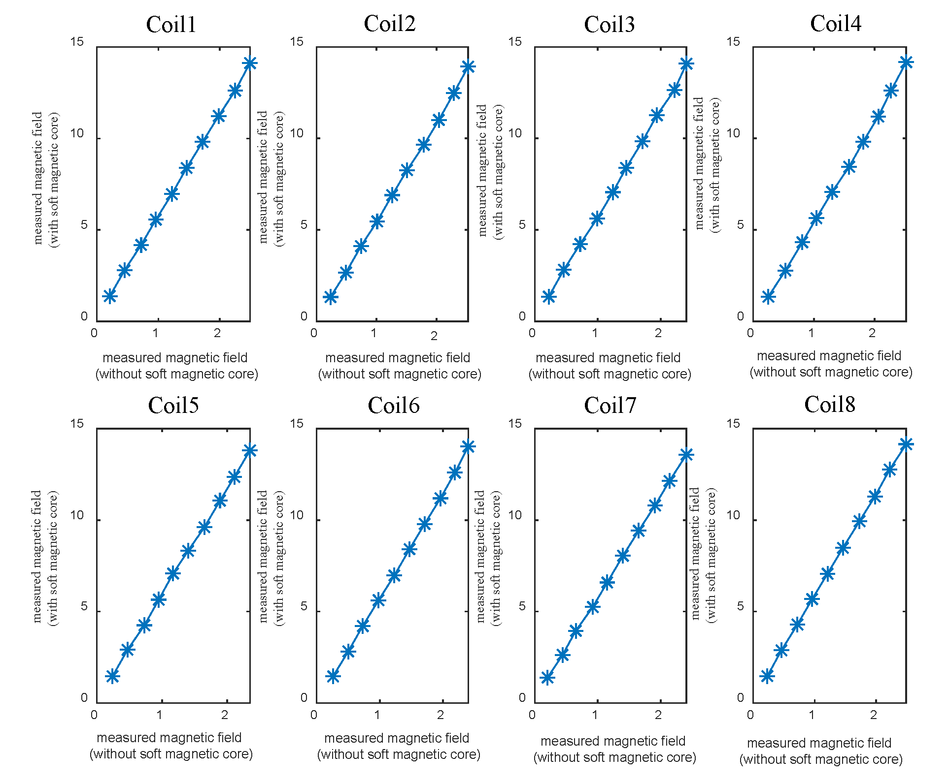
The mathematical model we have built describes the magnetic field distribution of the coil module without the soft magnetic core. The effect of the soft magnetic core on the spatial distribution of the magnetic field is characterized by the calibration of the magnetic field. The effect of the magnetic core on the spatial magnetic field distribution is divided into two parts. First, the magnetic core has an enhanced effect on the magnetic field excited by the coil itself; the literature [17] has verified the use of high-performance soft-magnetic material in the cores. Second, the coupling relationship between electromagnets. The magnetic field excited by an electromagnet after the current is applied can magnetize the magnetic core in the adjacent electromagnet so that the magnetic field distribution is nonlinear. For the first case, we study the change of the magnetic field strength at a fixed point when the input current increases linearly for a single-coil module (coil and core are assembled together). Figure 4 shows that the magnetic core in the eight-coil modules has a linear enhancement effect on the magnetic field distribution.The abscissa is the measured magnetic field generated by a single coil module without a soft magnetic core under different currents, and the ordinate is the magnetic field generated by a single coil module under different currents when a soft magnetic core is installed. The slope of the line connecting each scattered point and the origin of the coordinate system represents the enhancement coefficient of the magnetic field of the soft magnetic core under different input current conditions. The results in the figure show that a straight line passing through the origin of the coordinate system can be used to connect the scattered points and this characterizes the effect of the linear enhancement of the magnetic core in the workspace.

For the second case, the coupling effect of the magnetic field is temporarily unable to be described in accurate mathematical terms. Our research idea is to collect the magnetic field data to separate the linear change data in the magnetic field from the non-linear change data due to the coupling effect and estimate the non-linear quantities using approximate mathematical language. Therefore, we conducted the following experiment. Collecting the magnetic field intensity distribution of a single module and module assembly at a series of points. When the test input current sets the maximum current of the system (10 A), the offset of the magnetic field value generated by the coupling effect reaches the maximum. The test data shows that the magnetic field value offset caused by the coupling effect of 61% test points in the global range is less than 0.1 mT, 94% is less than 0.2 mT, and the maximum offset value does not exceed 0.3 mT. Therefore, we can know that the bias caused by the magnetic field bias due to the coupling effect at most points in the workspace is negligible compared to other errors introduced in the microrobot control model, such as approximate mathematical descriptions in dynamic modeling.

We tested the magnetic field strength of eight rectangular electromagnetic coils at a point in the workspace with or without a magnetic core. The magnetic field magnification of the eight coils constitutes an $8\times 8$ diagonal matrix $K_r$, which acts as a coefficient matrix of the current vector to compensate for the difference in the individual electromagnetic coils.

2.4. Mathematical Model of the Set of Coils

We have considered the following two points when designing the system configuration. First, we are more concerned with the force control of milli/microrobots, which is related to the gradient of the field, compared to the torque control. Second, the focus of the paper is on the potential of rectangular coils for remote control applications of milli/microrobots. The choice to be consistent with one typical configuration will allow for a comparison of system performance and experimental results with the previous system (Octomag). The magnetic milli/microrobot needs at least eight stationary electromagnets to obtain the desired torque and force at any point in the workspace. To date, a variety of manipulation systems have been developed, in terms of the generation of a spatial derivative in the field, which corresponds to force-generation capability, the Octomag configuration is the strongest [28].

Eight rectangular electromagnetic coils have been used to build a rectangular electromagnetic coil set actuation platform. The numbering sequence divided into two groups is shown in Figure 5. Since the actuation system does not have a priority level for each control direction of the milli/microrobot, there is no difference between the upper and lower sets of electromagnetic coil designs. For an isotropic system, eight electromagnetic coils are distributed around the Z-axis angle of 45 degrees considering the symmetry of the upper and lower groups, while the upper and lower coils and the Z-axis form an angle of 45 degrees and 90 degrees, respectively. Each electromagnetic coil acts as an independent magnetic field generating device. The central axis of the long axis of each coil intersects at a point, that is, the global coordinate system origin. The origin of the local coordinate system of the single-coil is separated from the global coordinate origin by 165 mm. The size of a single coil is 48 mm × 48 mm × 200 mm, which is l = 100 mm, w = 24 mm, h = 24 mm in the magnetic field mathematical model.

Using the measured calibration values for the respective electromagnet, the magnetic field and gradient of the rectangular coil set in the workspace can be calculated through homogeneous transformation matrix, which will provide a basis for generating the milli/microrobot actuation matrix. According to the coil set design layout, the origin of the global coordinate system is $R_{off}={\left[\begin{array}{ccc}{X}_{off}& Y_{off}& Z_{off}\end{array}\right]}^T={\left[\begin{array}{ccc}0.165& 0& 0\end{array}\right]}^T$ ($mm$) in the local coordinate system of a single rectangular electromagnetic coil. Equations (15) and (16) is the transformation matrix of the global coordinate system to the local coordinate system of the magnetic actuation system.

The position of the point in the global coordinate system under the local coordinate system of each coil is obtained by solving the above equation. The magnetic induction intensity and gradient at a unit current are obtained by using the magnetic field model of the rectangular electromagnetic coil, and then the magnetic induction intensity and the gradient component for the superposition operation in the global coordinate system are obtained by the inverse rotation matrix.

$$\begin{array}{cc}\hfill T{R}_{\delta }& =\left[\begin{array}{cc}{R}_z\left(\epsilon \right)& R_{off}\\ 0& 1\end{array}\right]\hfill \end{array}$$

(15)

For $\delta =(1;2;3;4)$, $\epsilon =(-3\pi /4;3\pi /4;\pi /4;-\pi /4)$.

$$\begin{array}{cc}\hfill T{R}_{\delta }& =\left[\begin{array}{cc}{R}_y(-\pi /4)R_z\left(\epsilon \right)& R_{off}\\ 0& 1\end{array}\right]\hfill \end{array}$$

(16)

For $\delta =(5;6;7;8)$, $\epsilon =(-\pi /2;-\pi ;\pi /2;\pi )$.

Where $R_x\left(\alpha \right)\in SO\left(3\right)$ is the rotation matrix around X axis of the global coordinate system by an angle $\left(\alpha \right)$; $R_y\left(\beta \right)\in SO\left(3\right)$ is the rotation matrix around Y axis of the global coordinate system by an angle $\left(\beta \right)$; $R_z\left(\gamma \right)\in SO\left(3\right)$ is the rotation matrix around Z axis of the global coordinate system by an angle $\left(\gamma \right)$.

As the capacity of the maximum current output is 10 A, the magnetic field flux density can reach approximately 15 mT when a single coil is sourced. When the other coils are considered, the magnetic field flux density can reach a magnitude of 35 mT. Obviously, the minimum value of magnetic field flux density in the work area is 0 mT.

3. Modeling and Control

3.1. Milli/Microrobot Dynamic Analysis

In the actuation process, in addition to actuation by an external force $F_m$ applied by the magnetic field, the milli/microrobot is also subjected to liquid viscous forces $F_d$ that opposes its direction of motion, as well as $F_g$ and buoyancy forces $F_b$ in the liquid environment. The electrostatic force and Van der Waals force have a weak influence on the milli/microrobot motion compared with the above-mentioned main forces [28,29,30,31,32] by considering the milli/microrobot’s millimeter-scale shape. As a result, they both have been ignored in order to simplify the dynamic model, which is shown as follows:

$$F_m+F_d+F_g+F_b=ma$$

(17)

The liquid viscous force $F_d$ of the milli/microrobot in the liquid environment can be approximated as:

$$F_d=-\frac{1}{2}{\rho }_f{(v-v_f)}^{2}A{C}_d$$

(18)

where v of is the moving speed the milli/microrobot, $v_f$ is the liquid flow velocity, ${\rho }_f$ is the fluid density, A is the front-end area when the milli/microrobot moving, and $C_d$ is the drag coefficient, which can be estimated as follows:

$$C_d=\frac{24}{R_e}+\frac{6}{1+\sqrt{R_e}}+0.4$$

$$R_e=\frac{{\rho }_f(v-v_f)L}{{\mu }_f}$$

where $R_e$ is the Reynolds number, ${\mu }_f$ is the dynamic viscosity coefficient of the fluid, L represents the characteristic length of the milli/microrobot.

The milli/microrobot in a liquid environment receives its own buoyancy force in the vertical direction. The calculation formula is expressed by Equation (19), where V represents the volume of the milli/microrobot and $\rho$ represents the material density of the milli/microrobot.

$$F_g+F_b=V(\rho -{\rho }_f)g$$

(19)

From the above analysis, (19) can be rewritten as (20), where $k_x$, $k_y$, $k_z$ are constant coefficients determined by the milli/microrobot in the actual working environment.

$$\begin{array}{cc}\hfill m\left(\begin{array}{c}{a}_x\\ a_y\\ a_z\end{array}\right)=& \left(\begin{array}{c}{F}_{mx}\\ F_{my}\\ F_{mz}\end{array}\right)+\left(\begin{array}{c}0\\ 0\\ -V(\rho -{\rho }_f)g\end{array}\right)\hfill \\ \hfill & +\left(\begin{array}{ccc}-k_x& 0& 0\\ 0& -k_y& 0\\ 0& 0& -k_z\end{array}\right)\left(\begin{array}{c}{(v-v_f)}_x^2\\ {(v-v_f)}_y^2\\ {(v-v_f)}_z^2\end{array}\right)\hfill \end{array}$$

(20)

Control the milli/microrobot to move along a particular trajectory which can be divided into calculating the required magnetic field and gradient at discrete points on the trajectory in real-time. An example is shown in Figure 6. The milli/microrobot moves along the planned spatial curve trajectory called “mountain climbing” motion from the starting point in three-dimensional space, and the main force analysis at each point is indicated by different color arrows.

3.2. Milli/Microrobot Magnetic Actuation Algorithm

The torque and force that the milli/microrobot should be subjected to at point P can be realized based on the mapping relationship between the magnetic field contribution and the driven current vector. Assuming that the magnetic field generated at point P by the $e_{th}$ coil in the unit current in the global coordinate frame is expressed as $B_e\left(P\right)$. The magnetic field flux density $B\left(P\right)$ generated at point P with eight electromagnetic coils can be represented as follows.

$$\begin{array}{cc}\hfill B\left(P\right)& =\sum _{e=1}^8{B}_e\left(P\right)i_e\hfill \\ \hfill & =\left(\begin{array}{ccc}{B}_1\left(P\right)& \cdots & B_8\left(P\right)\end{array}\right)\left(\begin{array}{c}{i}_1\\ ⋮\\ i_8\end{array}\right)=\beta I\hfill \end{array}$$

(21)

The gradient component of the magnetic field generated by the electromagnetic coil set along the coordinates is:

$$\frac{\partial B}{\partial i}=\left(\begin{array}{ccc}\frac{\partial B_1}{\partial i}& \cdots & \frac{\partial B_8}{\partial i}\end{array}\right)\left(\begin{array}{c}{i}_1\\ ⋮\\ i_8\end{array}\right)={\beta }_{i}I$$

(22)

where $i=x,y,z$. The torque and force of the milli/microrobot at position P in the workspace can be expressed by the actuation Equation (23), where $A_{(T,F)}\left(M\right)$ is a $6\times 8$ actuation matrix.

$$\left(\begin{array}{c}T\\ F\end{array}\right)=\left(\begin{array}{c}{S}_k\left(M\right)\beta \\ M^T{\beta }_x\\ M^T{\beta }_y\\ M^T{\beta }_z\end{array}\right)\left(\begin{array}{c}{i}_1\\ ⋮\\ i_8\end{array}\right)=A_{T,F}\left(M\right)I$$

(23)

For a milli/microrobot, the desired torque and force that the magnetic field needs to apply are determined and the current vector of the electromagnetic coil set can be obtained by (21). Since the system is over-actuated, the current vector that satisfies the above conditions is not unique. This is a convex optimization problem, and the objective function and constraints are set according to the actual requirements [33]. All movements of the milli/microrobot can be equivalent to the superposition of fixed-point actuation and linear motion actuation assuming that the milli/microrobot moves very slowly. Considering that the energy consumption and heat generation of the system are linear with the quadratic of the coil current, the objective functions in both motion states are set to the minimum of the Euclidean norm of the current vector. The constraints are derived from the deformation of the actuation equation according to the actual actuation requirements and system characteristics and it is mainly divided into two parts as shown below. These two linear optimizations are performed in the Gurobi Optimizer.

3.2.1. Fixed-Point Actuation

As shown in Algorithm 1, it is essential that the magnetic moment direction of the milli/microrobot is consistent with the magnetic field in the workspace under the action of the magnetic torque. At the same time, the magnetic field gradient in the local area is insufficient to generate the magnetic force for moving the position of the milli/microrobot. The inequality constraint of the current vector is set according to the current rating range of the actual actuation current source, which is determined by the actual actuation performance of the power system.

Algorithm 1 Optimization for Fixed-point Actuation

Input:$B_{des}\in {\mathbb{R}}^3$, $F_{des}\in {\mathbb{R}}^3$ Result:$I\in {\mathbb{R}}^3$ Objective Function:$minf\left(i\right)={\sum }_{i=1}^8{i}_i^2$ Subject to: $\beta I=B_{des}$ $\left(\begin{array}{c}{M}^T{\beta }_x\\ M^T{\beta }_y\\ M^T{\beta }_z\end{array}\right)I\le F_{des}$ $0\le i_n\le I_{max}$ End

3.2.2. Displacement Actuation

As shown in Algorithm 2, the displacement of the milli/microrobot is controlled by changing the magnetic field gradient in the case where the magnetic moment of the milli/microrobot is in the same direction as the magnetic field. The key to the displacement actuation of the milli/microrobot is to consider the force of the milli/microrobot in the liquid environment and accurately control the force it receives. To decouple rotation DOF and translation DOF, the direction of the magnetic field is set to the desired orientation of the milli/microrobot (the direction of the magnetic moment of the milli/microrobot assuming the milli/microrobot is a magnetic carrier) so that the milli/microrobot exerts the desired torque simultaneously.

Algorithm 2 Optimization for Displacement Actuation

Input:$B_{des}\in {\mathbb{R}}^3$, $F_{des}\in {\mathbb{R}}^3$ Result:$I\in {\mathbb{R}}^3$ Objective Function:$minf\left(i\right)={\sum }_{i=1}^8{i}_i^2$ Subject to: $\beta I\ge B_{des}$ $\left(\begin{array}{c}{M}^T{\beta }_x\\ M^T{\beta }_y\\ M^T{\beta }_z\end{array}\right)I=F_{des}$ $0\le i_n\le I_{max}$ End

4. Experiments and Results

4.1. System Implementation

Based on the coil set layout model proposed in Section 2, the Rect3D (see Figure 7) has been established. The electromagnet cores are made of H125, which is an FeNi alloy produced by Hengdian Group DMEGC Magnetics CO.,LTD (Dongyang city, Zhejiang province, China).Its saturation magnetization is on the order of 1500 mT, and the initial permeability is 125 H/m. Each core has a length of 30 mm, width of 30 mm and height of 30 mm. Each coil is assembled with ten cores.

The power control unit is composed of a host PC and eight DC programmable power supplies, respectively, connected to the corresponding coils on the electromagnetic actuation platform. The host computer and the DC programable power supply are connected through the USB serial port, and the I/O interface control of the program control instrument is realized by using the VISA function library developed by the NI company. SCPI (Standard Commands for Programmable Instruments) command format is used to realize remote communication between the host computer and the DC power supply. The camera has a resolution of $640\times 480$. Its visual standard protocol supports the Directshow protocol and Twain protocol. The camera lens uses a large multiple continuous zoom lens with an optical magnification of 0.13 ∼ 2 times and a working distance of 65 ∼ 700 mm.

The software part of the milli/microrobot magnetic actuation system includes the magnetic actuation algorithm, the power driver, the milli/microrobot real-time recognition program, and the implementation of a UI control interface. In part of the mathematical model of the spatial magnetic field distribution, the spatial magnetic field model of the rectangular electromagnetic coil combination is built by C ++ on the Qt Creator platform and is packaged into a class, which mainly includes the magnetic field solving method of the rectangular electromagnetic coil under the local coordinate system and the absolute coordinate system. The magnetic field model is used to obtain the magnetic field at the point of the absolute coordinate system of the rectangular electromagnetic coil. Combined with the milli/microrobot magnetic actuation algorithm, the mapping relationship between the magnetic field torque and the force to the input current is established. Gurobi is used to solve linear programming problems of actuating milli/microrobot based on rectangular electromagnetic coils, which can get calculation results faster and more accurately. In addition, we implemented the magnetic actuation algorithm on the Qt Creator platform to apply the Gurobi function library interface to meet the solution requirements.

Experiments were performed to demonstrate the developed system and actuation strategy. The first thing to declare is that the microrobot manufactured here is a model of the system’s function demonstration. In the experimental part of the article, we choose a magnetic carrier with a regular shape to simplify dynamic modeling or reduce the impact of dynamic modeling errors on system evaluation. In order to simulate the movement of the milli/microrobot in human body fluid, the working space is filled with methyl silicone oil, of which the kinematic viscosity is 500 $cst$ and the density is 0.97 g/cm${}^3$. The magnetic carrier was put in the acrylic cube placed in the $XOY$ plane of the workspace, as shown in Figure 6c. A visual feedback system, as shown in Figure 6b, consists of two industrial cameras mounted vertically to obtain image information of the working plane $XOY$ and $XOZ$. The image of the magnetic carrier was captured through image processing, and the geometrical center of the magnetic carrier was used to define the position.

4.2. Open Loop Control Results

Open-loop experiment operation process. First, preset the motion trajectory, then reversely solve the current sequence according to the mapping relationship between the current and the magnetic field distribution, and finally input the current sequence to record the motion trajectory of the milli/microrobot.

We initially demonstrated that the magnetic carrier can be manipulated by fixed-point rotating under the open-loop control which can visually characterize the control accuracy of the system in the direction of the magnetic field B. The origin of the global coordinate system $(X=0$ mm, $Y=0$ mm, $Z=0$ mm) was selected for performing experiments and fixed-point rotation experiments around the Z-axis are performed as shown in Figure 8. The purpose of this experimental demonstration is mainly to show that the system allows us to decouple degrees of freedom for rotation and translation. The orientation of the milli/microrobot converges at one point in the trajectory, and at the same time, the trajectory of its centroid point is a circle in the plane. Therefore, the two-DOF orientation motion and three-DOF translational motion of the milli/microrobot are decoupled.

Table 2. Experimental Results.

Data	1	2	3	4	5	6	7	8	9	10	11	12
Desired Angle (${}^{\circ }$)	15	30	45	60	75	90	105	120	135	150	165	180
Measured Angle (${}^{\circ }$)	13.9	29.3	44.7	57.8	76.2	89.4	105.8	119.7	133.7	149.7	164.3	179
Error (${}^{\circ }$)	1.1	0.7	0.3	2.2	−1.2	0.6	−0.8	0.3	1.3	0.3	0.7	1.0

illustrates the experimental results of the fixed-point rotation (a) and the errors in each situation.

In the second experiment, as shown in Figure 9 we verify that the system has the ability to provide a stable direction-determining force and the magnetic carrier moving along two different diagonal lines are performed which can intuitively characterize the accuracy of the magnetic field gradient direction control.

4.3. Closed Loop Control Results

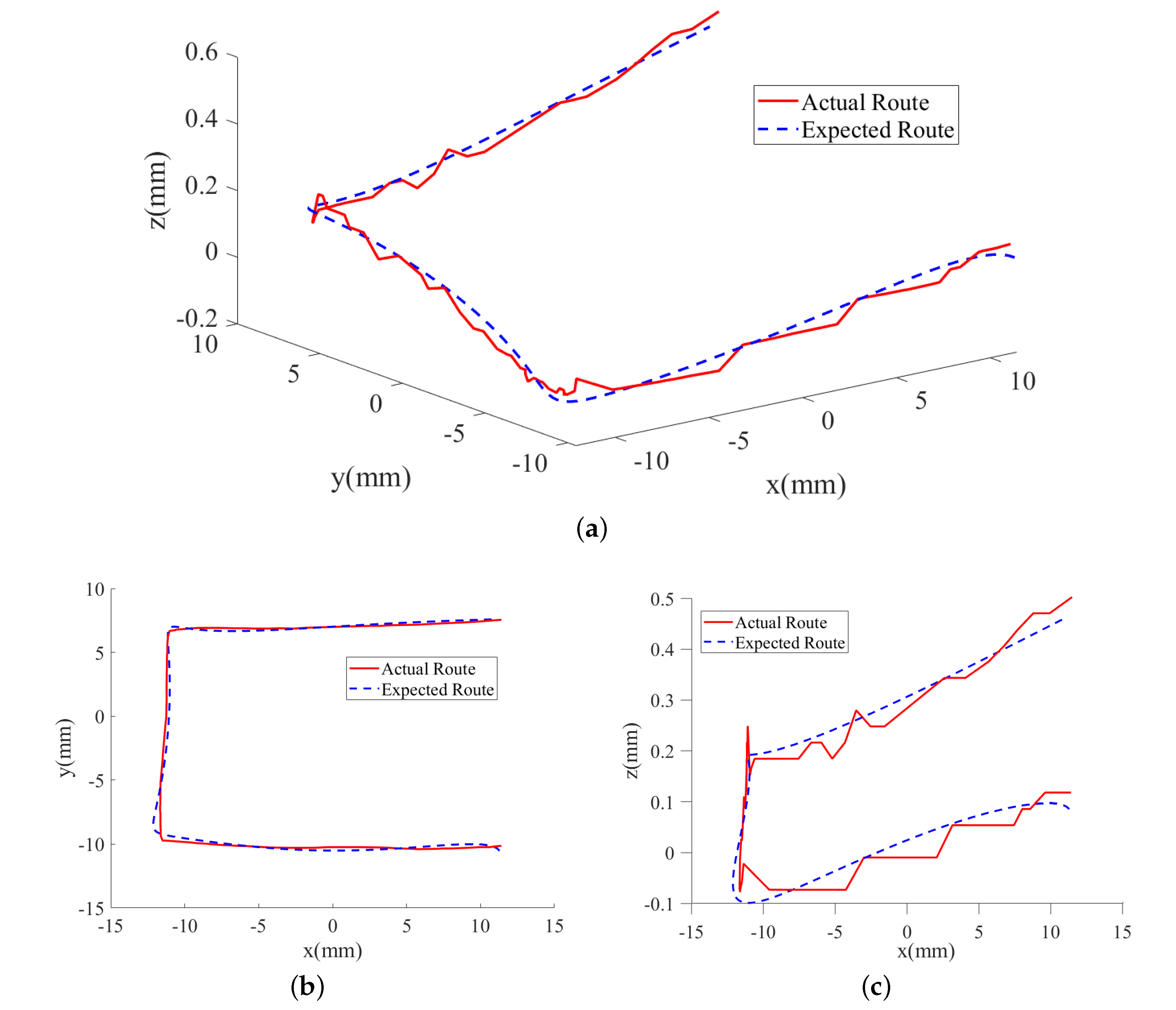
We further performed experiments of moving the magnetic carrier along the predesigned trajectory path under closed loop control. Figure 10 shows the moving sequence at different time instants, viewed from both top and the side of the workspace. Figure 11 shows 3D motion trajectory. As shown in Figure 12, the average errors of trajectory tracking were 0.44 mm.

4.4. Discussion

Here, we describe an analysis of position control error in open-loop control. Because there is no capture of the spatial position of the milli/microrobot, the results of the open-loop experiments depend on the initial position of the milli/microrobot. If the initial position of the milli/microrobot deviates from the initial position of the preset trajectory, it will cause a large deviation in the trajectory. Due to the randomness of the deviation between the initial position and the preset initial position of the micro-robot in the “up stair” and “down stair” movements, the error performance in these two cases is random (no correlation).

Theoretically, the larger the characteristic size (e.g., length, radius) of the magnetic carrier, the easier it is to be manipulated by the system. However, for medical scene applications, the millimeter-level and sub-millimeter-level dimensions are requirements for the design and manufacture of microrobots. Therefore, we use a cylindrical magnetic carrier with a diameter of 1 mm and a height of 1 mm in our experiments. The experimental results show that the system can achieve the manipulation of magnetic carriers of millimetre-level. If the size of the magnetic carrier is further reduced, the error of its posture control will increase.

5. Conclusions

In this study, we designed a milli/microrobot magnetic actuation system based on the rectangular electromagnetic coil to solve the actuation control problem of a milli/microrobot in the field of minimally invasive diagnosis and treatment. The mathematical model of the electromagnetic coil is used to construct the milli/microrobot actuation equation, so as to establish the mapping relationship between the torque and magnetic force of the milli/microrobot and the driven current of the coil set, and the linear programming algorithm is used to solve the driven current matrix. The three-dimensional coordinates of the milli/microrobot can be obtained in real-time through the visual feedback system, and the precise actuation of the milli/microrobot is realized. Experimental results show that the magnetic actuation system can realize the 5-DOF actuation of a milli/microrobot. Future work will improve the actuation performance of the magnetic actuation system to meet the needs of smaller magnetic milli/microrobots.

References

1. Nelson, B.J.; Kaliakatsos, I.K.; Abbott, J.J. Microrobots for Minimally Invasive Medicine. Annu. Rev. Biomed. Eng. 2010, 12, 55–85. [Google Scholar] [CrossRef] [PubMed] [Green Version]
2. Biomedical Applications of Untethered Mobile Milli/Microrobots. Proc. IEEE 2015, 103, 205–224. [CrossRef] [PubMed]
3. Ceylan, H.; Giltinan, J.; Kozielski, K.; Sitti, M. Mobile microrobots for bioengineering applications. Lab A Chip 2017, 17, 1705–1724. [Google Scholar] [CrossRef] [Green Version]
4. Li, J.; de Ávila, B.E.F.; Gao, W.; Zhang, L.; Wang, J. Micro/nanorobots for biomedicine: Delivery, surgery, sensing, and detoxification. Sci. Robot. 2017, 2, eaam6431. [Google Scholar] [CrossRef] [PubMed]
5. Ceylan, H.; Yasa, I.C.; Kilic, U.; Hu, W.; Sitti, M. Translational prospects of untethered medical microrobots. Prog. Biomed. Eng. 2019, 1, 012002. [Google Scholar] [CrossRef]
6. Rahmer, J.; Stehning, C.; Gleich, B. Remote magnetic actuation using a clinical scale system. PLoS ONE 2018, 13, e0193546. [Google Scholar] [CrossRef] [Green Version]
7. Atkinson, I.C.; Renteria, L.; Burd, H.; Pliskin, N.H.; Thulborn, K.R. Safety of human MRI at static fields above the FDA 8T guideline: Sodium imaging at 9.4 T does not affect vital signs or cognitive ability. J. Magn. Reson. Imag. Off. J. Int. Soc. Magn. Reson. Med. 2007, 26, 1222–1227. [Google Scholar] [CrossRef] [PubMed]
8. Zaremba, L.A. Guidance for Industry and FDA Staff: Criteria for Significant Risk Investigations of Magnetic Resonance Diagnostic Devices; Center for Devices and Radiological Health: Silver Spring, MD, USA, 2003. [Google Scholar]
9. Abbott, J.J.; Peyer, K.E.; Lagomarsino, M.C.; Zhang, L.; Dong, L.; Kaliakatsos, I.K.; Nelson, B.J. How should microrobots swim? Int. J. Robot. Res. 2009, 28, 1434–1447. [Google Scholar] [CrossRef]
10. Hu, W.; Lum, G.Z.; Mastrangeli, M.; Sitti, M. Small-scale soft-bodied robot with multimodal locomotion. Nature 2018, 554, 81–85. [Google Scholar] [CrossRef]
11. Tottori, S.; Zhang, L.; Qiu, F.; Krawczyk, K.K.; Franco-Obregón, A.; Nelson, B.J. Magnetic helical micromachines: Fabrication, controlled swimming, and cargo transport. Adv. Mater. 2012, 24, 811–816. [Google Scholar] [CrossRef]
12. Zhang, L.; Abbott, J.J.; Dong, L.; Kratochvil, B.E.; Bell, D.; Nelson, B.J. Artificial bacterial flagella: Fabrication and magnetic control. Appl. Phys. Lett. 2009, 94, 064107. [Google Scholar] [CrossRef] [Green Version]
13. Huang, H.W.; Sakar, M.S.; Petruska, A.J.; Pané, S.; Nelson, B.J. Soft micromachines with programmable motility and morphology. Nat. Commun. 2016, 7, 1–10. [Google Scholar] [CrossRef] [PubMed] [Green Version]
14. Khalil, I.S.; Fatih Tabak, A.; Klingner, A.; Sitti, M. Magnetic propulsion of robotic sperms at low-Reynolds number. Appl. Phys. Lett. 2016, 109, 033701. [Google Scholar] [CrossRef]
15. Mahoney, A.W.; Abbott, J.J. Five-degree-of-freedom manipulation of an untethered magnetic device in fluid using a single permanent magnet with application in stomach capsule endoscopy. Int. J. Robot. Res. 2016, 35, 129–147. [Google Scholar] [CrossRef]
16. Nam, J.; Lee, W.; Jung, E.; Jang, G. Magnetic navigation system utilizing a closed magnetic circuit to maximize magnetic field and a mapping method to precisely control magnetic field in real time. IEEE Trans. Ind. Electron. 2017, 65, 5673–5681. [Google Scholar] [CrossRef]
17. Kummer, M.P.; Abbott, J.J.; Kratochvil, B.E.; Borer, R.; Sengul, A.; Nelson, B.J. OctoMag: An electromagnetic system for 5-DOF wireless micromanipulation. IEEE Trans. Robot. 2010, 26, 1006–1017. [Google Scholar] [CrossRef]
18. Floyd, S.; Pawashe, C.; Sitti, M. An untethered magnetically actuated micro-robot capable of motion on arbitrary surfaces. In Proceedings of the IEEE International Conference on Robotics and Automation, Pasadena, CA, USA, 19–23 May 2008; pp. 419–424. [Google Scholar]
19. Diller, E.; Giltinan, J.; Lum, G.Z.; Ye, Z.; Sitti, M. Six-degree-of-freedom magnetic actuation for wireless microrobotics. Int. J. Robot. Res. 2016, 35, 114–128. [Google Scholar] [CrossRef]
20. Khalil, I.S.; Keuning, J.D.; Abelmann, L.; Misra, S. Wireless magnetic-based control of paramagnetic microparticles. In Proceedings of the 4th IEEE RAS & EMBS international conference on biomedical robotics and biomechatronics (BioRob), Rome, Italy, 24–27 June 2012; pp. 460–466. [Google Scholar]
21. Niu, F.; Li, J.; Ma, W.; Yang, J.; Sun, D. Development of an enhanced electromagnetic actuation system with enlarged workspace. IEEE/ASME Trans. Mechatron. 2017, 22, 2265–2276. [Google Scholar] [CrossRef]
22. Song, S.; Yu, H.; Ren, H. Study on mathematic magnetic field model of rectangular coils for magnetic actuation. In Proceedings of the IEEE 28th Canadian Conference on Electrical and Computer Engineering (CCECE), Halifax, NS, Canada, 3–6 May 2015; pp. 19–24. [Google Scholar]
23. Gu, H.; Song, S.; Zhang, Q.; Meng, M.Q.H. RectMag: An accurate magnetic field model based actuation system. In Proceedings of the IEEE International Conference on Robotics and Biomimetics (ROBIO), Qingdao, China, 3–7 December 2016; pp. 248–253. [Google Scholar]
24. Diller, E.; Sitti, M. Micro-scale mobile robotics. Found. Trends Robot. 2013, 2, 143–259. [Google Scholar] [CrossRef]
25. Jiles, D. Introduction to Magnetism and Magnetic Materials; CRC Press: Boca Raton, FL, USA, 2015. [Google Scholar]
26. Abbott, J.J.; Ergeneman, O.; Kummer, M.P.; Hirt, A.M.; Nelson, B.J. Modeling magnetic torque and force for controlled manipulation of soft-magnetic bodies. IEEE Trans. Robot. 2007, 23, 1247–1252. [Google Scholar] [CrossRef]
27. Nagy, Z.; Ergeneman, O.; Abbott, J.J.; Hutter, M.; Hirt, A.M.; Nelson, B.J. Modeling assembled-MEMS microrobots for wireless magnetic control. In Proceedings of the IEEE International Conference on Robotics and Automation, Pasadena, CA, USA, 19–23 May 2008; pp. 874–879. [Google Scholar]
28. Pourkand, A.; Abbott, J.J. A critical analysis of eight-electromagnet manipulation systems: The role of electromagnet configuration on strength, isotropy, and access. IEEE Robot. Autom. Lett. 2018, 3, 2957–2962. [Google Scholar] [CrossRef]
29. Dadkhah, M.; Kumar, N.; Yoon, J. Design and simulation of a 3D actuation system for magnetic nano-particles delivery system. In Intelligent Robotics and Applications, Proceedings of the International Conference on Intelligent Robotics and Applications, Busan, Korea, 25–28 September 2013; Springer: Cham, Switzerland, 2013; pp. 177–187. [Google Scholar]
30. Ghanbari, A.; Chang, P.H.; Nelson, B.J.; Choi, H. Electromagnetic steering of a magnetic cylindrical microrobot using optical feedback closed-loop control. Int. J. Optomechatron. 2014, 8, 129–145. [Google Scholar] [CrossRef]
31. Belharet, K.; Folio, D.; Ferreira, A. Control of a magnetic microrobot navigating in microfluidic arterial bifurcations through pulsatile and viscous flow. In Proceedings of the IEEE/RSJ International Conference on Intelligent Robots and Systems, Vilamoura, Portugal, 7–12 October 2012; pp. 2559–2564. [Google Scholar]
32. Arcese, L.; Fruchard, M.; Ferreira, A. Endovascular magnetically guided robots: Navigation modeling and optimization. IEEE Trans. Biomed. Eng. 2011, 59, 977–987. [Google Scholar] [CrossRef] [PubMed]
33. Boyd, S.; Boyd, S.P.; Vandenberghe, l. Convex Optimization; Cambridge University Press: Cambridge, UK, 2004. [Google Scholar]
Figure 1. Schematic diagram of three types of magnetic field actuation methods. Their movement trends are all from right to left. (a) Compound magnetic field actuation; (b) Rotating magnetic field actuation; (c) Oscillating magnetic field actuation.
Applsci 10 02677 g001
Figure 2. The proposed Rectmag3D prototype designed and constructed at Harbin Institute of Technology, Shenzhen. (a) Main mechanical structure of the system; (b) Top view of the main structure.
Applsci 10 02677 g002
Figure 3. Modeling of the rectangular coil. The coordinate system is based on the coil. The X-axis is along the length of the coil and the origin of the coordinate is at the center position of the coil. The model is based on the Biot–Savart Law and the superposition principle. The direction of the current I is different in the four different planes.
Applsci 10 02677 g003
Figure 4. The linear enhancement of the magnetic field distribution by the soft magnetic core in a single coil module.
Applsci 10 02677 g004
Figure 5. Rectangular electromagnetic coil set actuation platform model.
Applsci 10 02677 g005
Figure 6. Magnetic force simulation of each point when the milli/microrobot moves along the planned spatial curve trajectory. (a) Schematic diagram of force decomposition of magnetic carrier in motion along a predetermined trajectory. (b) Schematic diagram of changes in the magnetic force component during the magnetic carrier’s completion of the predetermined trajectory.
Applsci 10 02677 g006
Figure 7. Rectangular electromagnetic coil set actuation platform. (a) System setup. The power supply for the system is IT6942A produced by ITECHELECTRONIC CO., LTD and its response time is 100 ms. This power supply drive system can simultaneously operate eight electromagnetic coils with a full load of 15A. (b) Schematic diagram of the placement of the workspace. The size of the workspace is 37 × 37 × 25 mm 3 . (c) The overall shape of the microrobot is a cone with a radius of 1.25 mm and a height of 2 mm, and is designed with threads embedded in the cone. Such a structure makes it possible to advance forward and wear the obstruction in front of the movement when it is rotated about its central axis. A cylindrical hole with a diameter of 1 mm and a height of 1 mm at the bottom of the cone is used for assembling the magnetic carrier. Microrobots are made by aluminum 3D printing. This makes the microrobot body not subject to any torque and force under the magnetic field and has a low mass to facilitate driving. The magnetic carrier can realize movements such as translation and rotation under the action of an external magnetic field to provide power for the microrobot. (d) Assembly relationship between microrobot and magnetic carrier. (e) The magnetic carrier is a cylinder having a diameter of 1 mm and a height of 1 mm and is made of neodymium iron boron and a density of 7500 kg/m 3 . (f) Mounting position of the side camera. (g) Assembly diagram of the coil module. (h) FeNi alloy. The uppercase yellow English letters in the figure show the same thing.
Applsci 10 02677 g007
Figure 8. Demonstration of rotation control. (a) The magnetic carrier rotates around the Z-axis at the coordinate point (0, 0, 0), and the rotation amplitude is 15 degrees each time. (b) The magnetic carrier enable more complex spatial rotational motion. The direction of the magnetic moment of the magnetic carrier is 45 degrees from the Z-axis, and the circular rotation around the Z-axis is performed at coordinates (0, 0, 0).
Applsci 10 02677 g008
Figure 9. Demonstration of displacement control. (a) The milli/microrobot moves from the upper-right corner of the workspace along with the X O Y projection to the lower-left corner while descending stepwise in the Z-axis direction. Average trajectory-completion time: 10.83 s. (b) The milli/microrobot moves from the lower-right corner of the workspace along with the X O Y projection to the upper-left corner while rising stepwise in the Z-axis direction. Average trajectory-completion time: 14.4 s. The left figures are trajectories in the 3D workspace. The right figures show the errors between actual and desired trajectories.
Applsci 10 02677 g009
Figure 10. Demonstration of visual feedback control and the magnetic carrier completes a “mountain climbing” movement. Average trajectory-completion time: 23.43 s. The figure indicates the captured image in real-time that was processed gradation conversion, Gaussian filtering, binarization, expansion processing, finding contours and locating the contour center point. The blue line represents the predesigned trajectory, the red line represents the actual trajectory, and the green arrow represents the direction of movement of the magnetic carrier.
Applsci 10 02677 g010
Figure 11. (a) Motion trajectory of the controlled magnetic carrier. (b) Projection of the trajectory in the X O Y plane. (c) Projection of the trajectory in the X O Z plane.
Applsci 10 02677 g011
Figure 12. Position tracking error in the X-axis, Y-axis, Z-axis direction and total position error.
Applsci 10 02677 g012