Parking Space and Obstacle Detection Based on a Vision Sensor and Checkerboard Grid Laser

Abstract

The accuracy of automated parking technology that uses ultrasonic radar or camera vision for obstacles and parking space identification can easily be affected by the surrounding environment especially when the color of the obstacles is similar to the ground. Additionally, this type of system cannot recognize the size of the obstacles detected. This paper proposes a method to identify parking spaces and obstacles based on visual sensor and laser device recognition methods by installing a laser transmitter on the car. The laser transmitter produces a checkerboard-shaped laser grid (mesh), which varies with the condition encountered on the ground, which is then captured by the camera and taken as the region of interest for the necessary image processing. The experimental results show that this method can effectively identify obstacles as well as their size and parking spaces even when the obstacles and the background have a similar color compared to when only using sensors or cameras alone.

1. Introduction

The advancements of science and technology, coupled with the rapid improvement in the standard of living, have resulted in higher demand for intelligent vehicles. One such demand aspect of intelligent vehicles is the Automatic Parking System (APS). As a result of rapid developments in most cities around the world, parking spaces are becoming narrower, and parking a vehicle without the guidance of a third party is becoming quite problematic and takes too much time to accomplish even with a parking guide. However, with the rapid development of APS technology, this task will be accomplished with ease and with minimal time needed without a parking guide. This system uses sensors or cameras to assess the parking situation and automatically adjust the angle of the steering device to accomplish a successful parking process [1,2].

APS that use sensors like ultrasonic radar sensors to find parking spaces have the advantage of high-speed data processing and long detection distance, free from the influence of light. However, ultrasonic radar cannot distinguish the types of obstacles, and it is easy to misjudge when the ultrasonic radar scans low barriers or potholes on the ground [3,4].

In addition to the ultrasonic radar, the parking space can also be recognized by the use of camera vision. The advantage of the camera is that it can acquire a large amount of data about the surrounding environment and can detect inclined objects. However, it is greatly influenced by the surrounding environment, and the accuracy of the recognized obstacles on the ground is low in situations where the color of the obstacles is similar to the color of the ground. Additionally, monocular cameras cannot recognize the size of objects, and binocular cameras are more expensive and the algorithms more complex [5,6,7,8].

Another technology that APS uses for parking space recognition is the LiDAR sensing system. This technology was originally developed and used by the military. It detects the distance of the surrounding environment by launching a multi-beam pulsed laser rotating 360 degrees, and it can also draw a 3D map. However, as a result of the high cost of this technology, LiDAR with a low wire harness is used in vehicles, which comes with a decrease in resolution, making it susceptible to producing blind spots and resulting in safety concerns [9,10,11].

The multi-sensor fusion technique for APS as proposed by many researchers is to overcome the above shortcomings of the other technologies. However, the high cost of this technology coupled with the fact that it has not sufficiently matured hinder its adoption [12,13,14]. Additionally, the theory of parking space recognition rarely considers the general situation of the obstacles in the parking space, which can lead to inaccurate obstacle identification [15].

In order to solve the above challenges, a new parking space recognition scheme is proposed in this paper. A laser transmitter is added to the vision sensor system. A chessboard effect laser grid is presented on the ground by a laser emitter mounted on the vehicle, and the shape of the laser grid will change when there are obstacles on the ground. After these changes are captured by the camera, through image processing, the laser mesh region is taken as the region of interest. This method can effectively identify parking spaces and obstacles in parking spaces and significantly improve the recognition rate of sufficient parking spaces.

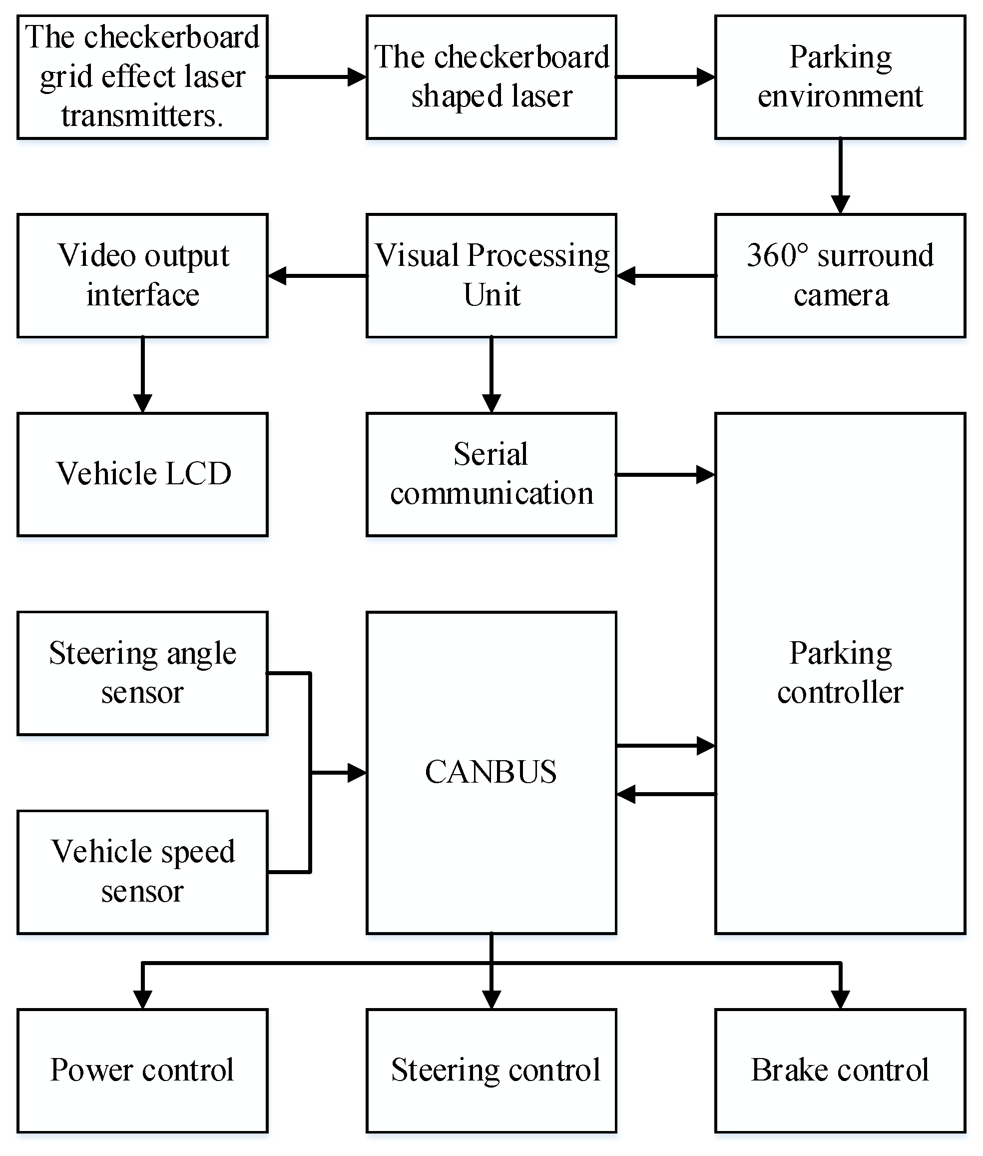
2. System Structure and Principle

The system structure of the parking space and obstacle detection based on the vision sensors and the laser device is shown in Figure 1. In addition to the original 360° camera sensors installed on the body of the vehicle, the system is also equipped with a checkerboard grid effect laser transmitter. The images of the parking space and the surrounding environment are captured by the 360° cameras. Then, the visual processor carries out the subsequent image processing and connects with the parking controller through the communication serial port.

The principle of the system is shown in Figure 2. The laser emitting devices are illuminated on the ground to present the shape of the checkerboard grid. When obstacles exist on the ground, such as vehicles in the parking space, the shape of the laser mesh will change. Similarly, when there are obstacles such as stones, potholes, walls, and floor locks on the ground, the laser mesh will produce different changes. The cameras capture the changes of the laser mesh, making it easier to recognize the parking spaces and the obstacles from images. As a result, the recognition efficiency and success rate will be improved. Furthermore, when parking at night, the laser emitting devices can emit light autonomously, which reduces the requirements for lighting conditions. In addition, the safety and applicability of the parking system will be improved.

After acquiring the environment image of the parking space, the system first preprocesses the image, which mainly includes gamma conversion image enhancement, image graying, mean filtering by smoothing and denoising, and binarized edge detection. Then, the region of interest will be extracted. After that, contour detection and convex hull detection are performed in the region of interest. Finally, the contour and convex hull will be displayed in the images. The algorithm flow is shown in Figure 3.

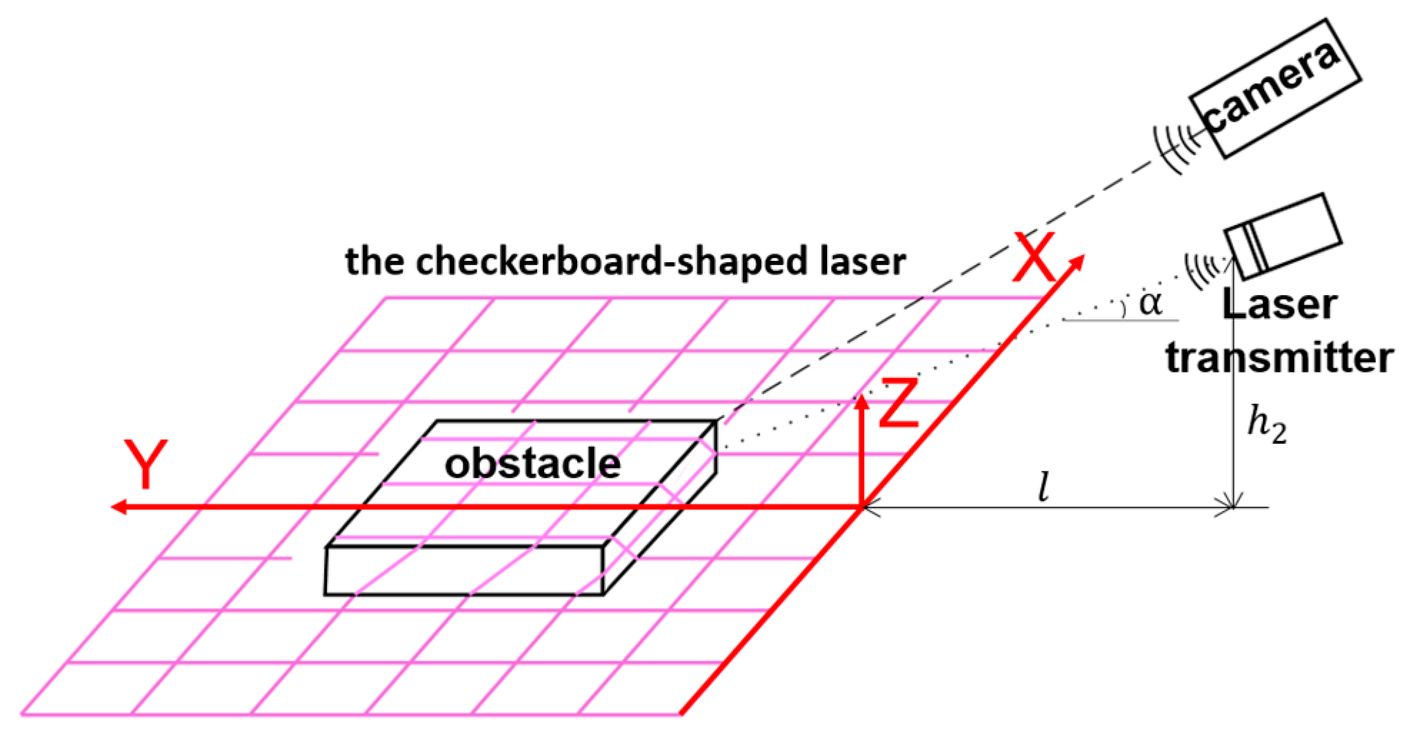
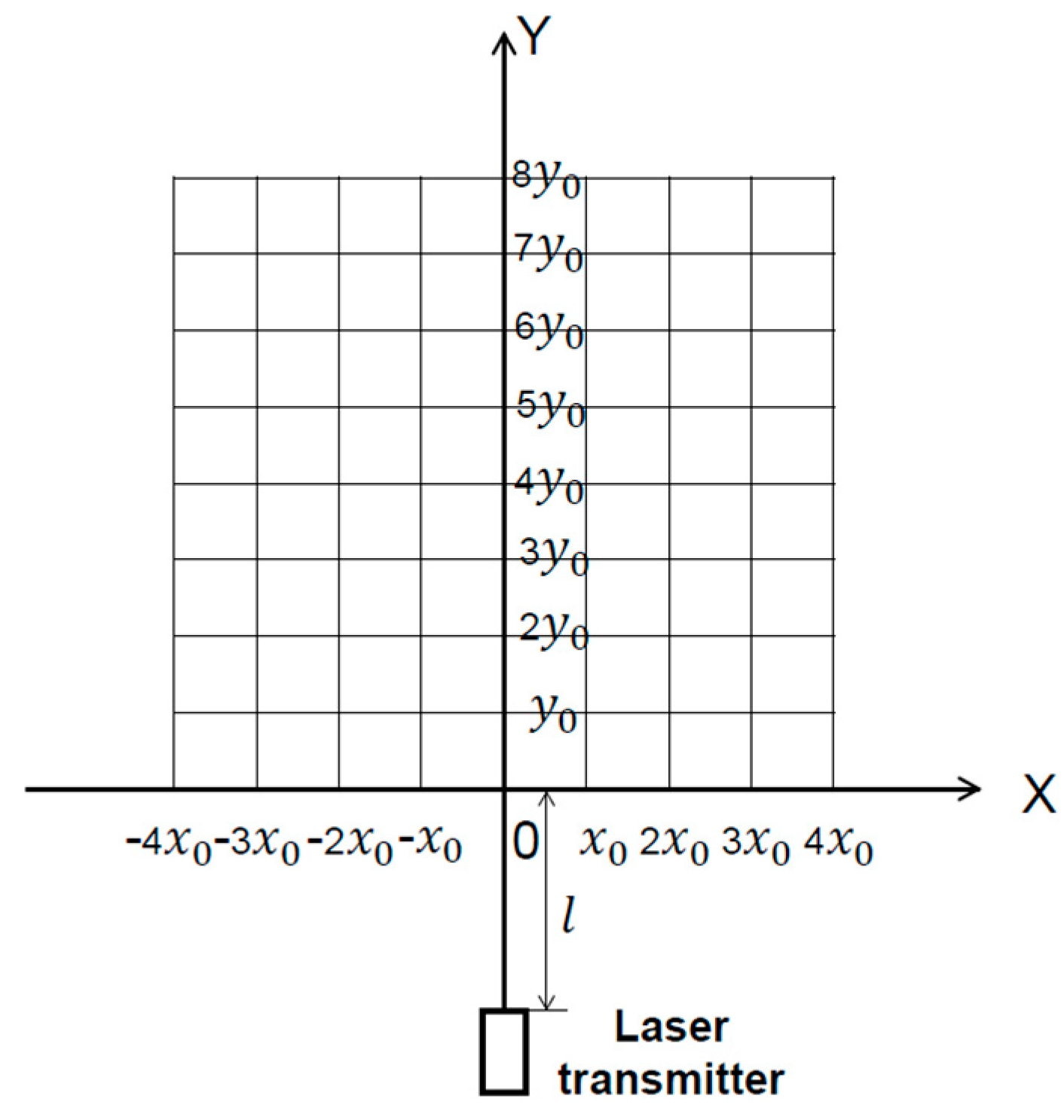
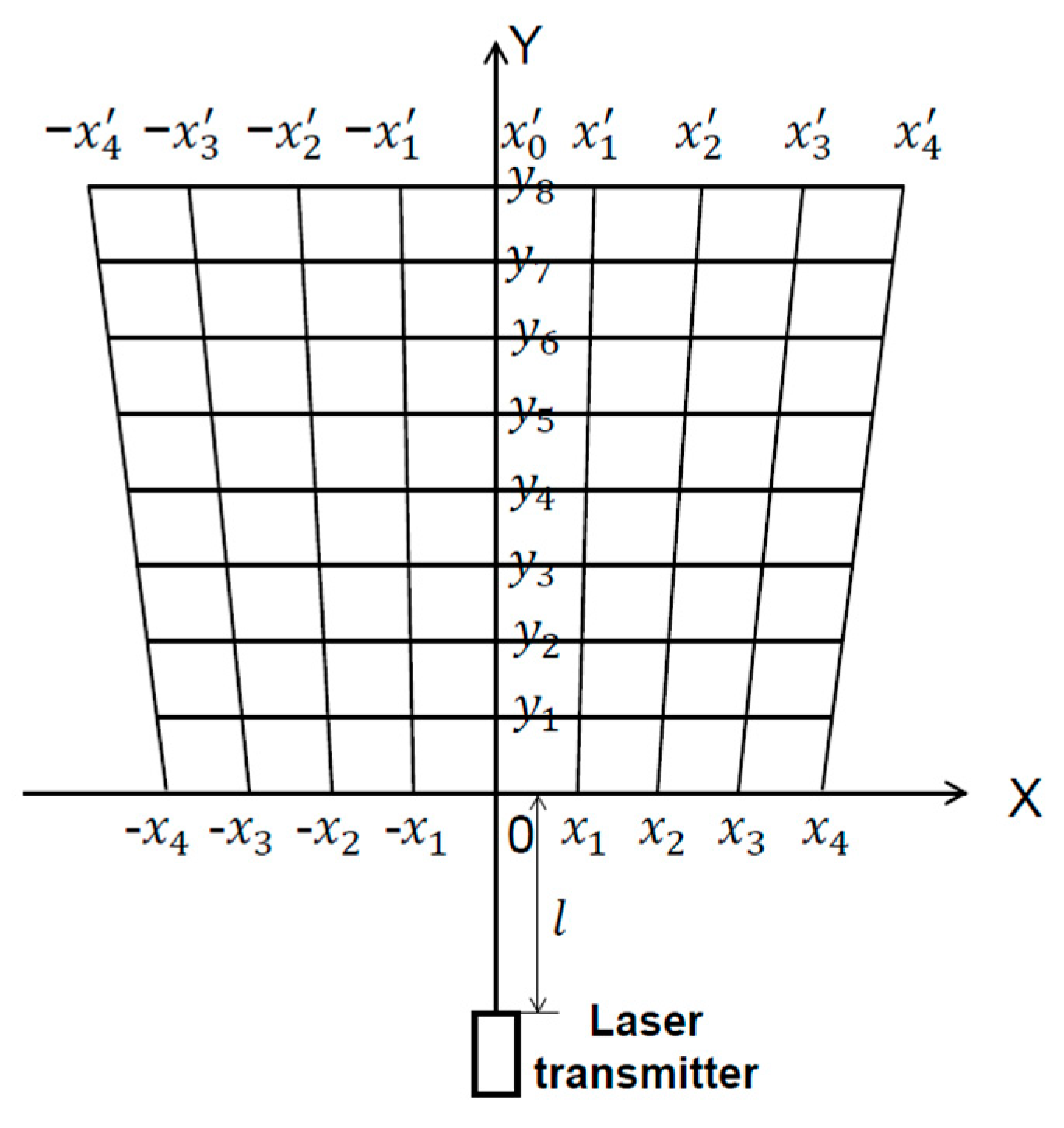
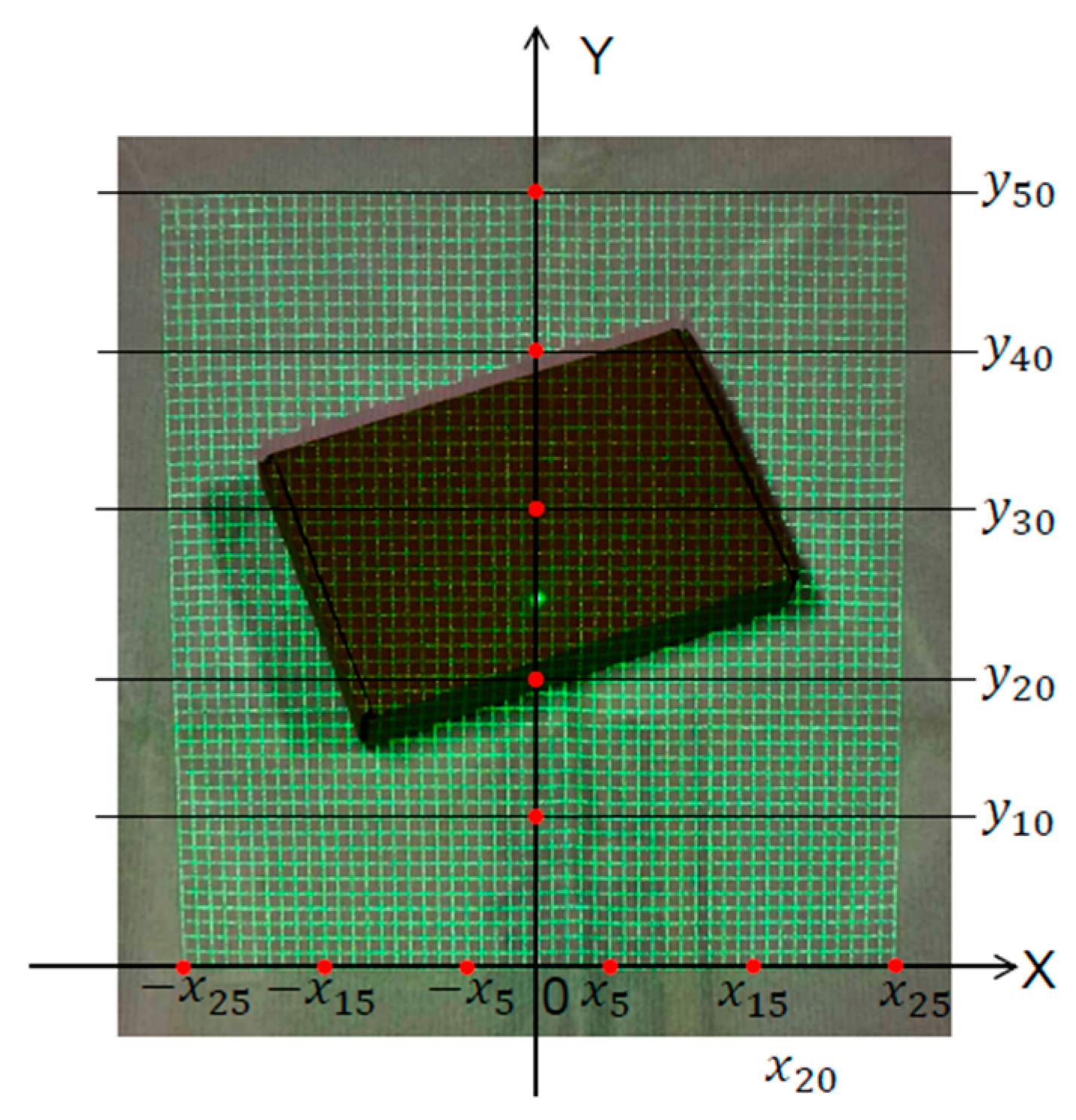
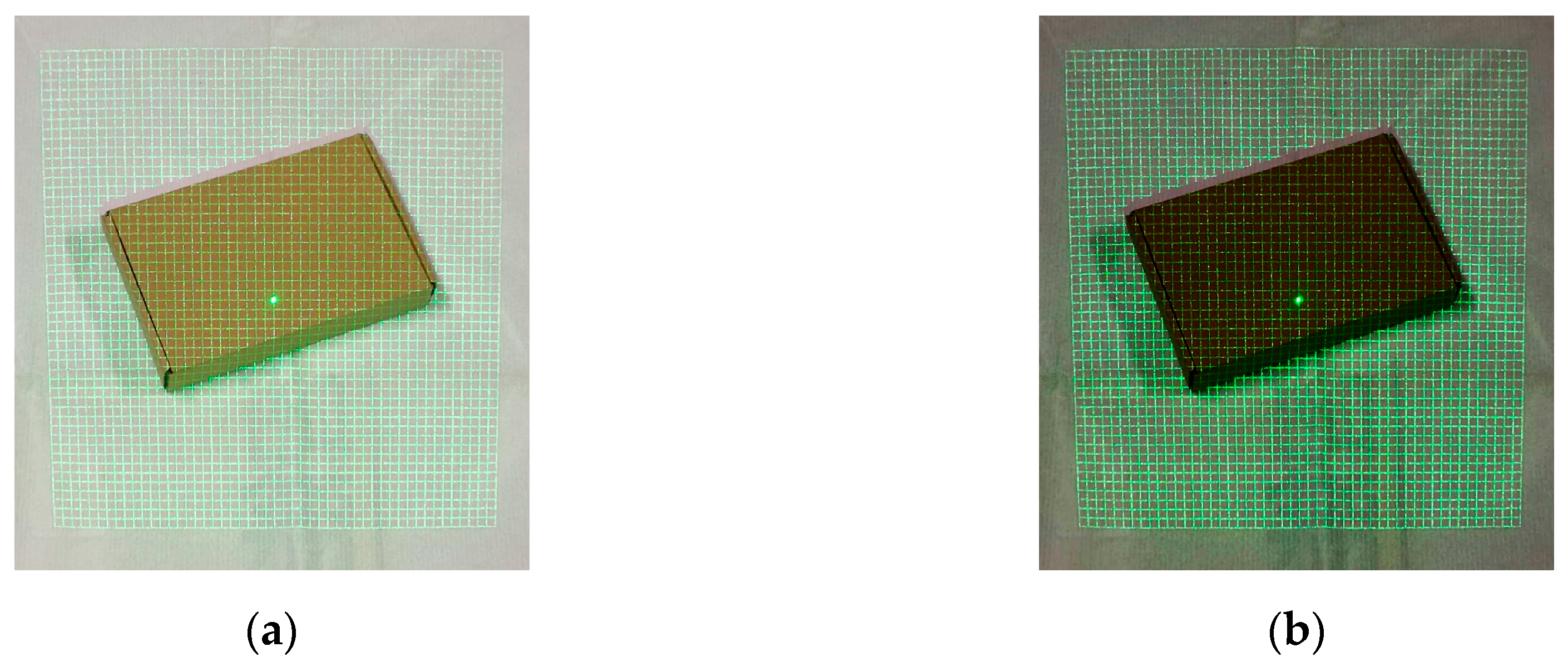
2.1. Realization of Checkerboard Laser Grid

The effect of the grid laser emitter on the ground is shown in Figure 4. The laser emitter illuminates the ground to present a checkerboard grid effect, and the laser line in the grid will change shape when illuminating obstacles on the ground. Moreover, the cameras can capture these shape changes for further image processing or machine learning to identify obstacles. Due to the high brightness, high directivity, and high monochromaticity of the laser, when the camera captures the laser mesh, the corresponding filter or the corresponding color detection in image processing can improve the capture of the special detection of the mesh and reduce the amount of image processing in the later stage.

As shown in Figure 4, the laser emitter is obliquely irradiated to the ground; the center line of the laser emitter is at α degrees to the horizontal plane; the laser emitter is at h₂ above the horizontal ground; and the distance between the laser emitter and the checkerboard laser grid is l.

As shown in Figure 5, in an ideal case, the laser emitter is illuminated on the level ground, presenting a uniformly distributed laser grid with a single grid length of x₀, and the width is y₀. In reality, the laser grid is deformed by the laser emitter tilted on the ground.

As shown in Figure 6, the laser network is an 8×8 grid; the laser line closest to the laser transmitter is the X-axis, and the central axis of the laser network is the Y-axis. The vertical distance between the flat laser line and the origin is 0, y₁, y₂, …, y₈, respectively. Due to the deformation of the vertical laser line, the endpoint is from −x₄, −x₃, …, 0, …, x₃, x₄ to −x₄’, −x₃’, …, 0, …, x₃’, x₄’. Therefore, the X-direction of each grid is changed to:

$$x_{ci}=\frac{\left|{x_i}^{\prime }-x_i\right|}{8},(i=1,2,3,4)$$

(1)

Furthermore, the coordinates of each grid intersection can be calculated when the obstacle appears in the laser grid. The coordinate range of the obstacle according to the position of the deformation can also be evaluated.

As shown in Figure 7, the coordinates of the rectangular obstacles in the figure are: (−x₁₂, y₁₄), (−x₁₉, y₃₃), (x₁₁, y₄₂), (x₁₈, y₂₅).

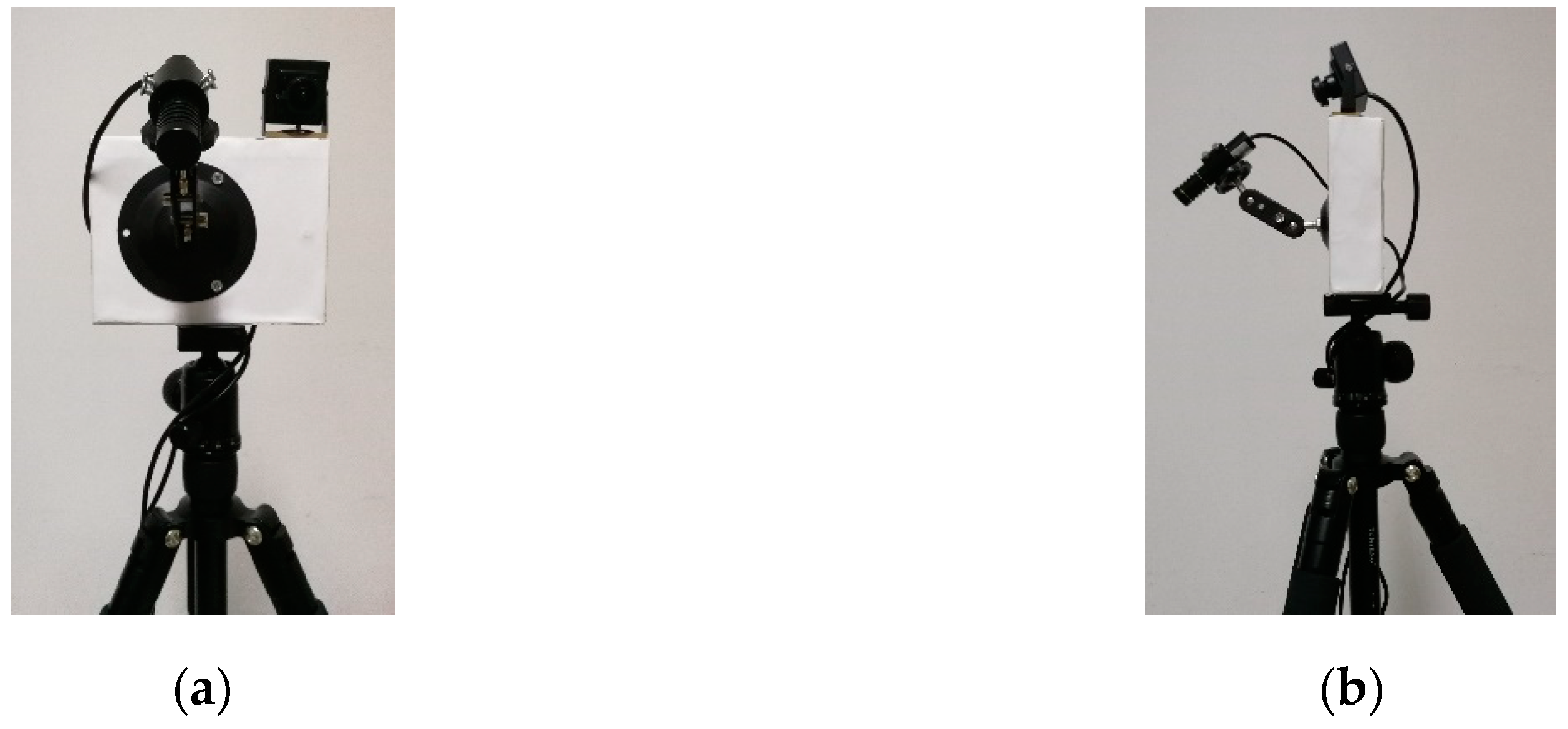
2.2. Image Acquisition

The image is captured by 360° cameras. The 360° cameras are equipped with four camera components mounted on the front, rear, left, and right sides of the car. When installing the cameras, the front camera is installed on the logo or the grill, and the rear camera is installed near the license plate light or trunk handle, as close as possible to the central axis. Left and right cameras are installed under the left and right rearview mirrors. The number and position of the cameras can also be adjusted according to the actual situation. Wide-angle cameras can be used, which can take complete environmental images around the vehicle at the same time. Images of the surrounding environment are simultaneously collected through the 360° cameras. After the image correction and image mosaicking, a 360° image is formed [16].

Camera Calibration

The calibration of the cameras mainly involves the transformation of four coordinate systems: world coordinate system, camera coordinate system, image plane coordinate system, and image pixel coordinate system. The calibration methods mainly include the Zhengyou Zhang calibration method [17], the RAC (Radial Alignment Constraint) two-stage method of Tsai, and the DLT (Direct Linear Transform) method [18,19,20].

Using a given known calibrator, the external parameter rotation matrix of camera R, translation matrix T, principal point coordinates of parametric images (C_x, C_y), the height and width of a single-pixel S_x, S_y, focal length f, and distortion factor k can be calculated.

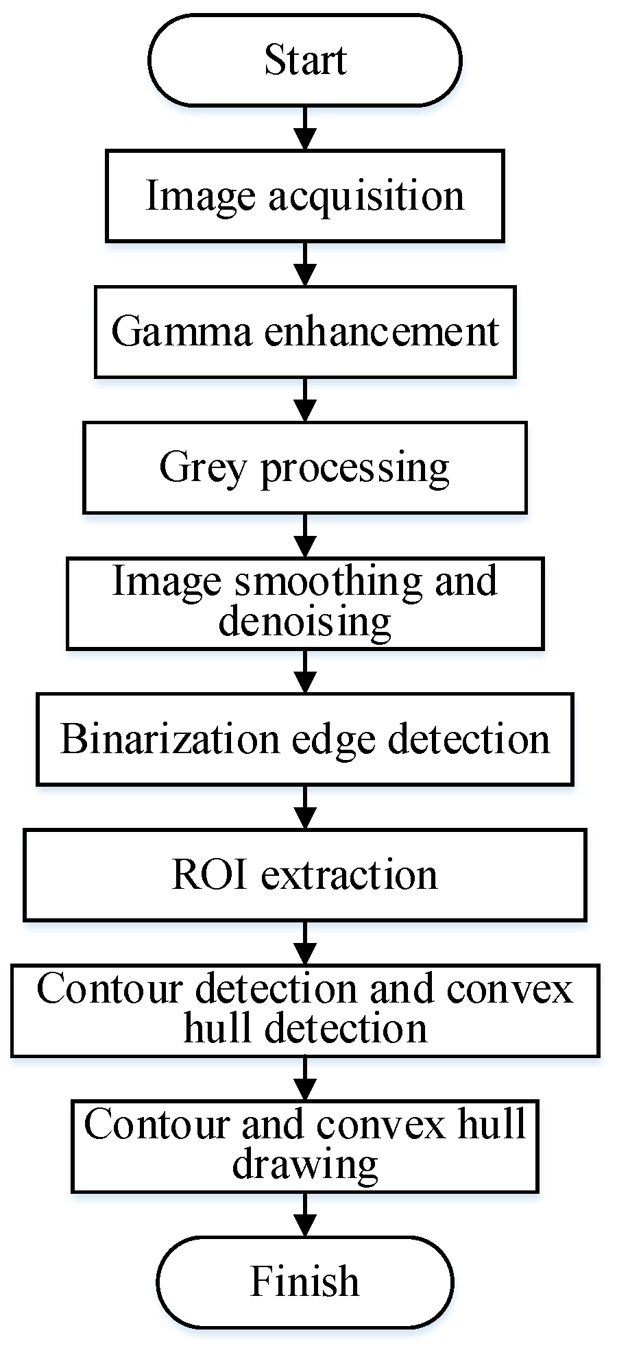
3. Image Preprocessing

The image acquired by the camera is affected by the surrounding noise and the environment, so that the target object to be recognized is not highly distinguishable from the surrounding environment image and cannot be directly used. Therefore, there is a need for image preprocessing of the original image.

3.1. Grayscale Processing

The process of transforming a color image into a gray image is called gray processing of the image. According to the principle of the three primary colors of red, green, and blue, any color F can be mixed with different ratios of R, G, and B.

$$F=r[R]+g[G]+b[B]$$

(2)

The color depth of a pixel in a gray image is called the gray value. The difference between a grayscale image and a black-and-white image is that the grayscale image contains the concept of color depth, which is the gray level. Since the color image has three channels and the gray image has only one channel, the processing speed for the color image is slow compared to the gray image. The grayscale processed image can greatly reduce the amount of subsequent calculation, and the information contained in the grayscale image is enough for calculation and analysis.

The image can be converted into a grayscale image by decomposing the color of color pixels into R, G, and B components using the following formula.

$$F(x,y)=0.299\times R(x,y)+0.587\times G(x,y)+0.114\times B(x,y)$$

(3)

When all the pixels in the color image are transformed by the above formula, the color image will be converted into a grayscale image [21].

3.2. Smoothing and Denoising of Images

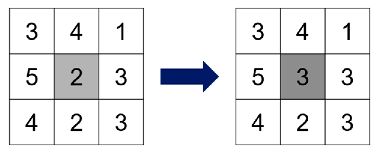
In the process of acquiring and transmitting the image can be affected by noise. This noise causes the image quality to degrade and can mask some of the characteristics of the image, which have the potential to make the analysis of the image difficult. While removing noise from the target image, it is also necessary to retain the details of the original image as much as possible, and the quality of the processing will directly affect the effectiveness and reliability of subsequent image processing and analysis. Commonly used methods for smoothing and denoising include mean filtering, median filtering, bilateral filtering, and Gaussian filtering [22].

Mean Filtering

In this paper, the smoothing and denoising method of mean filtering is adopted. The mean filtering is a typical linear filtering algorithm, which can help eliminate the sharp noise of images and realize image smoothing and blurring.

The mean filtering algorithm replaces the pixel points in the image by selecting an appropriate template operator and replaces the gray value of the pixel with a weighted average of the gray pixel values in its neighborhood. After smoothing and denoising by means of the mean filter algorithm, image f(i, j) is transformed into image g(x, y), and the equation is:

$$g(x,y)=\frac{1}{M}{\displaystyle {\sum }_{i,j\in S}f}(x,y)$$

(4)

In the formula, M is the total number of pixels, including the current pixel in the template. Generally, the template operators are m × m. If the template operator is 3 × 3, the total number of template pixels M is nine. The central pixel value is calculated using the following formula:

$$S=\frac{1}{9}{\displaystyle {\sum }_{i=1}^9{a}_i}$$

(5)

As shown in Figure 8, after the mean filtering, the value of the center pixel becomes:

$$S=\frac{3+4+1+5+2+3+4+2+3}{9}=3$$

(6)

3.3. Image Enhancement Technology

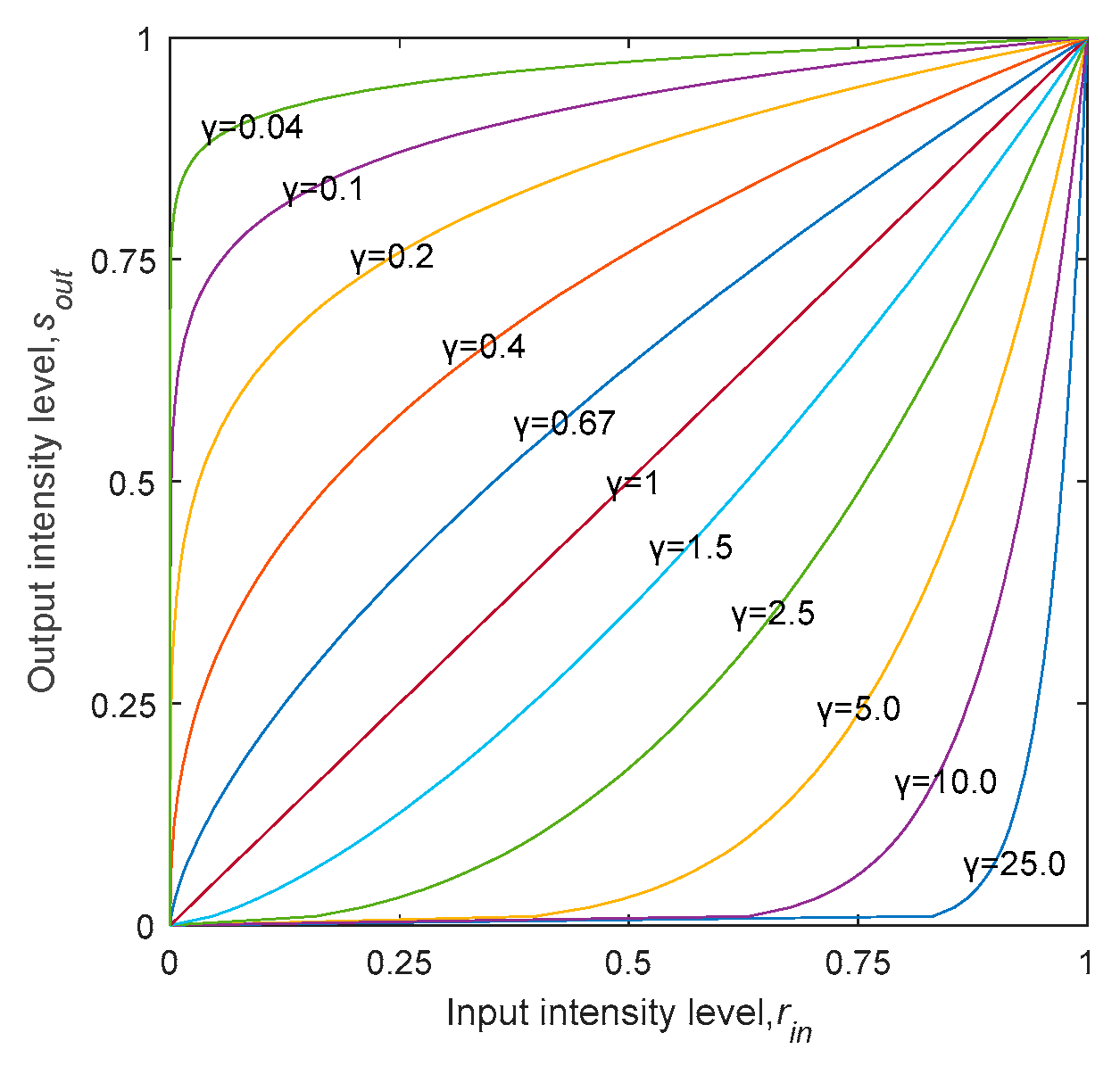
Image enhancement is necessary to either improve the image quality or the image interpretation and recognition effect by emphasizing the overall or local characteristics of the image. The commonly used techniques in image enhancement include histogram equalization, Laplacian, log transform, gamma transform, and image enhancement based on the fuzzy technique [23].

Gamma Transform

The gamma transform is the enhancement technique that is adopted in this paper. It is mainly used for image correction, and the image with too high a gray level or low a gray level is corrected to enhance contrast and image detail [24]. The formula is as follows:

$$S_{out}=c{r_{in}}^r$$

(7)

where r_in is the pixel value of the image, which is a non-negative real number, and c is called the grayscale scaling coefficient, used for the overall stretched image grayscale, which is a constant, whose value ranges from zero to one, usually taking a value of one.

The correction effect of the gamma transform on the image is achieved by enhancing the details of the low gray or high gray scale, as shown in Figure 9. It can be intuitively understood from the gamma curve: γ takes one as the dividing line. When γ < 1, the intensity of light increases, and the extension effect on the low gray part of the image is enhanced, which is called gamma compression; when γ > 1, the expansion effect on the high gray portion of the image is enhanced, and the illumination intensity is weakened, which is called gamma expansion. Therefore, by taking different gamma values, the effect of enhancing the details of the low or high gray levels can be achieved. In general, the image enhancement effect of gamma transform is evident when the image contrast is low and the overall brightness value is high.

As shown in Figure 10a,b, since the original image is too bright, it is difficult to separate the laser grid from the background. After the gamma conversion, the contrast of the image is greatly improved. The features of the laser grid are shown more clearly, which reduces the amount of processing in the next step.

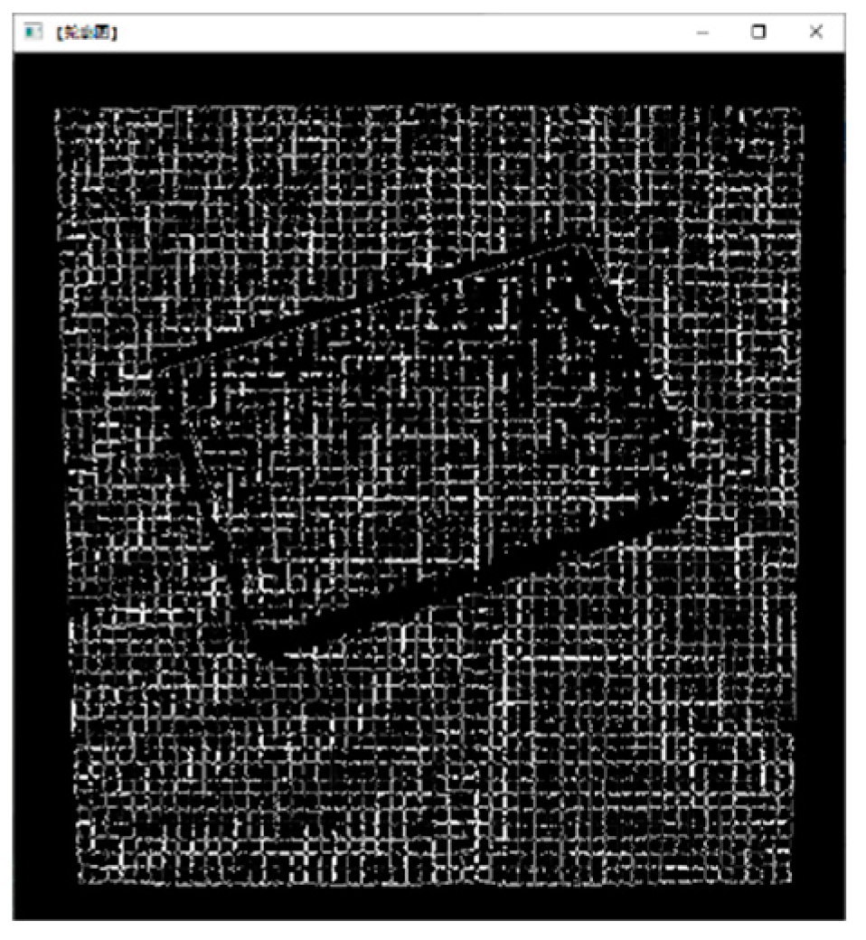
3.4. Image Binarization

The representation of an image with the visual effects of only black and white is known as image binarization. This process reduces the amount of data in the image in order to highlight the contour of the target object and to separate it from the boundary. This is accomplished by applying a threshold on the image, which can be adjusted to observe the specific features of the target object in the image.

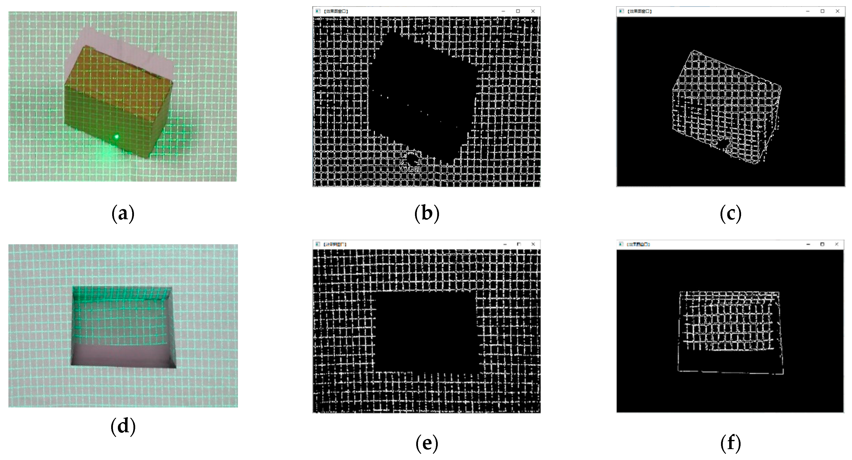
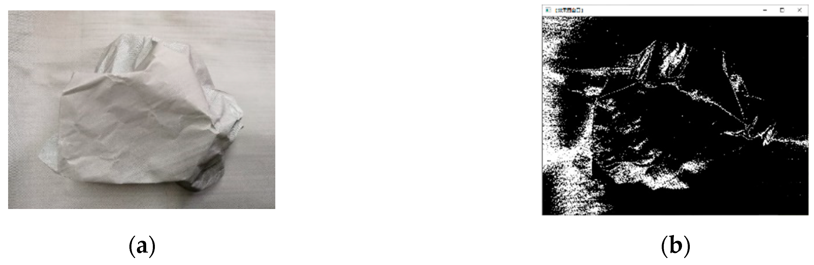
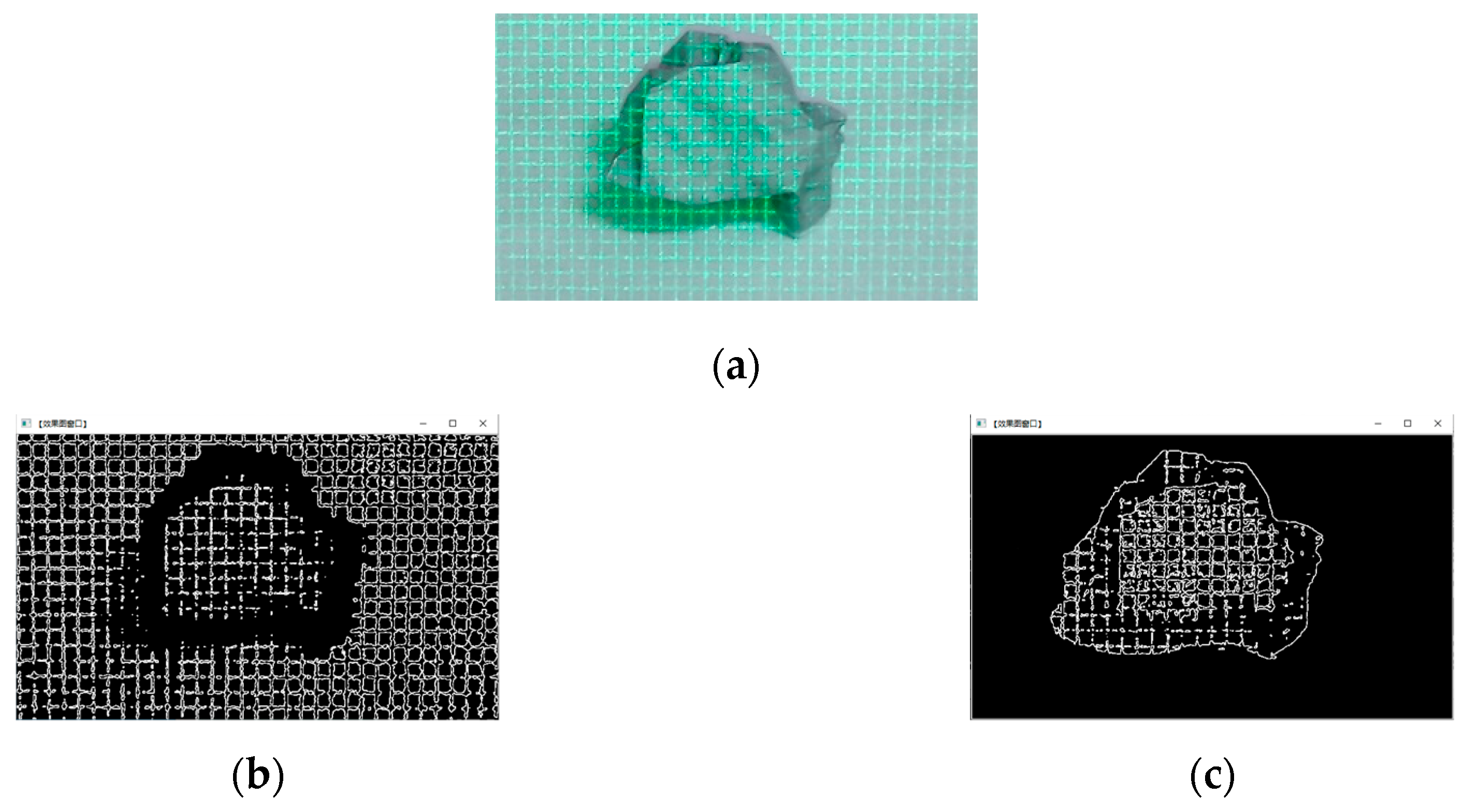
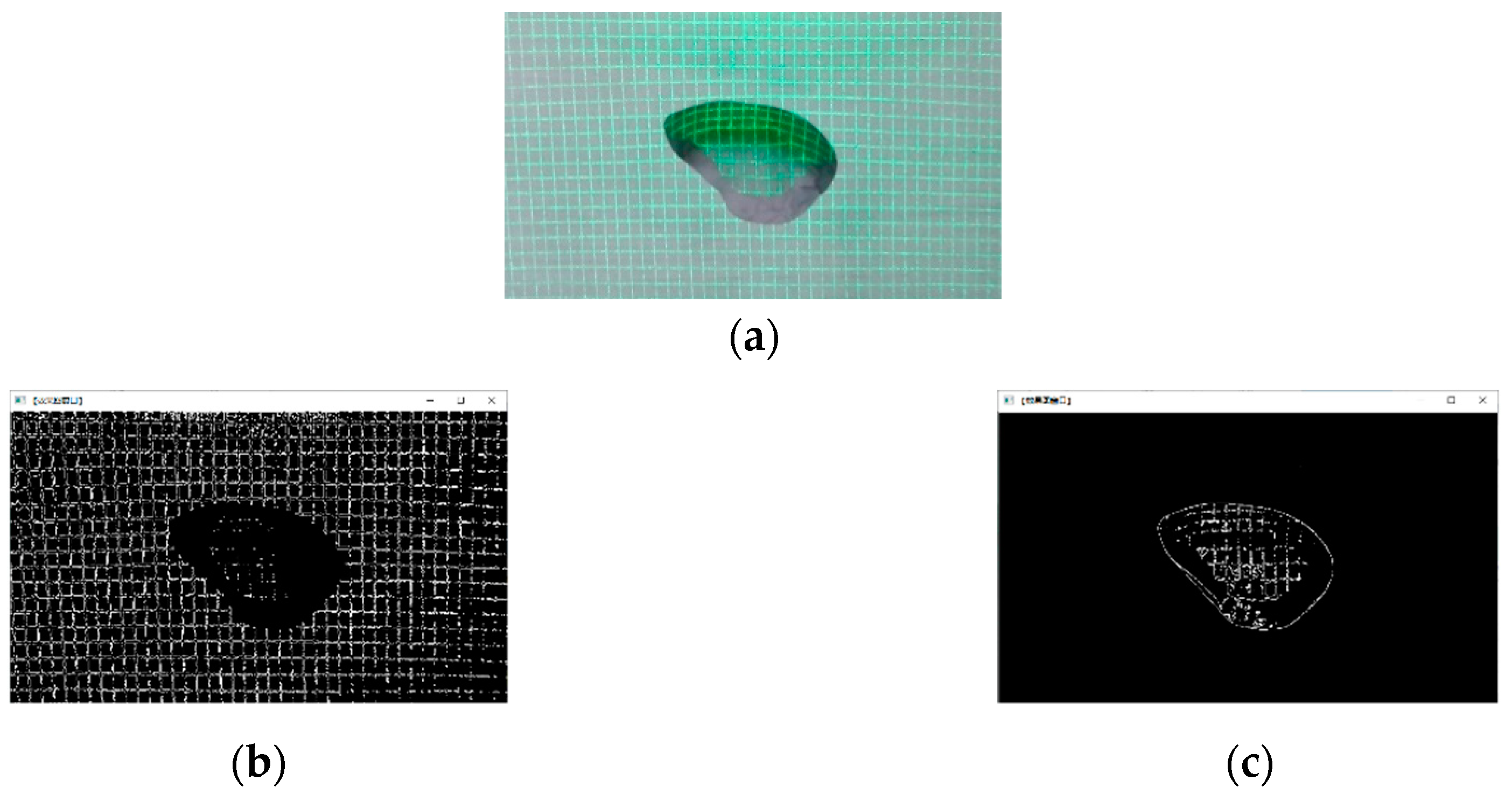
4. Feature Extraction and Recognition of Obstacles

Changes in the laser grid indicate a potential obstacle on the ground. This deformation region is then taken as the region of interest (ROI), and the necessary image processing is then applied to filter out the ROI for obstacle recognition.

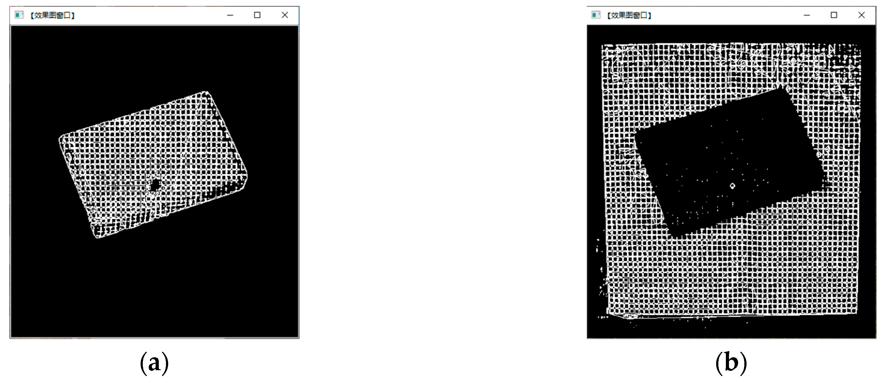
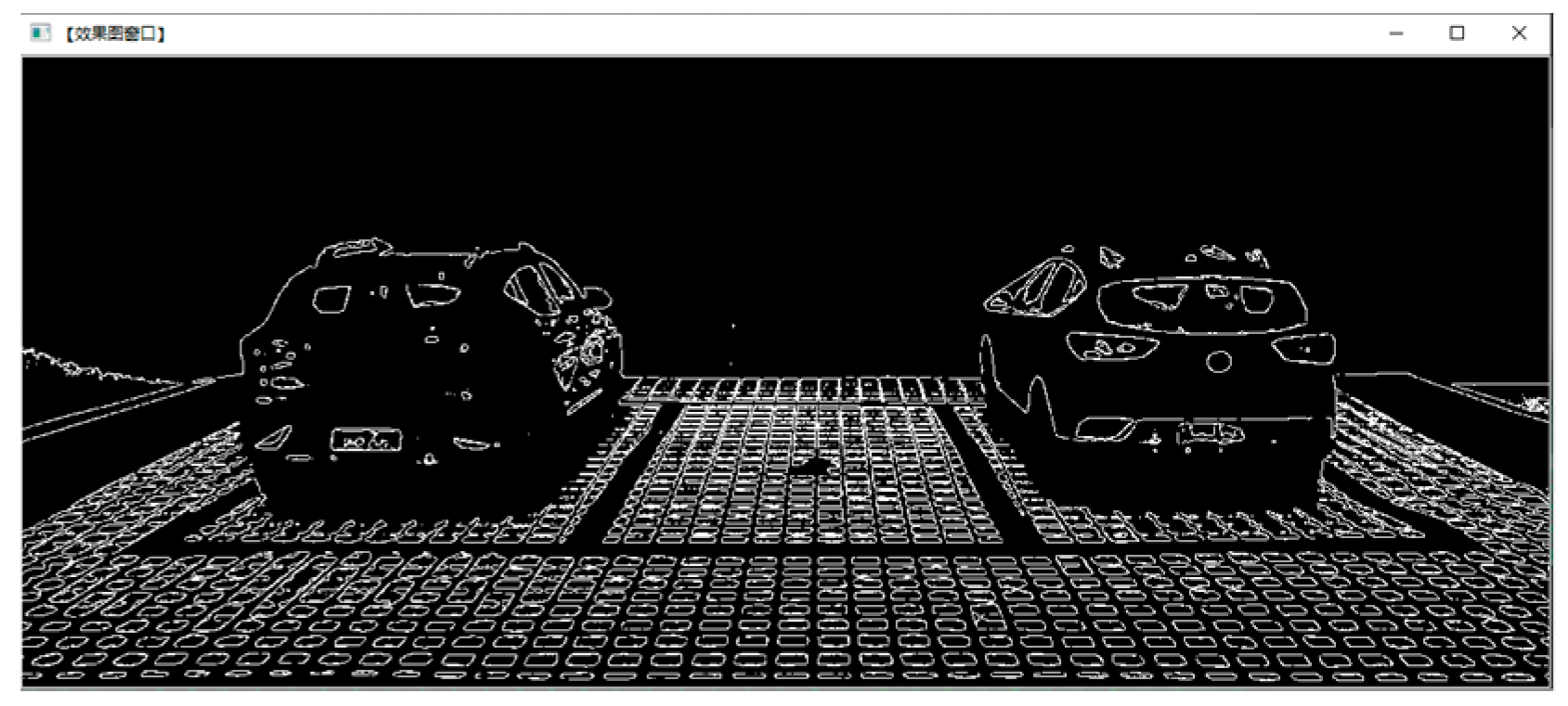
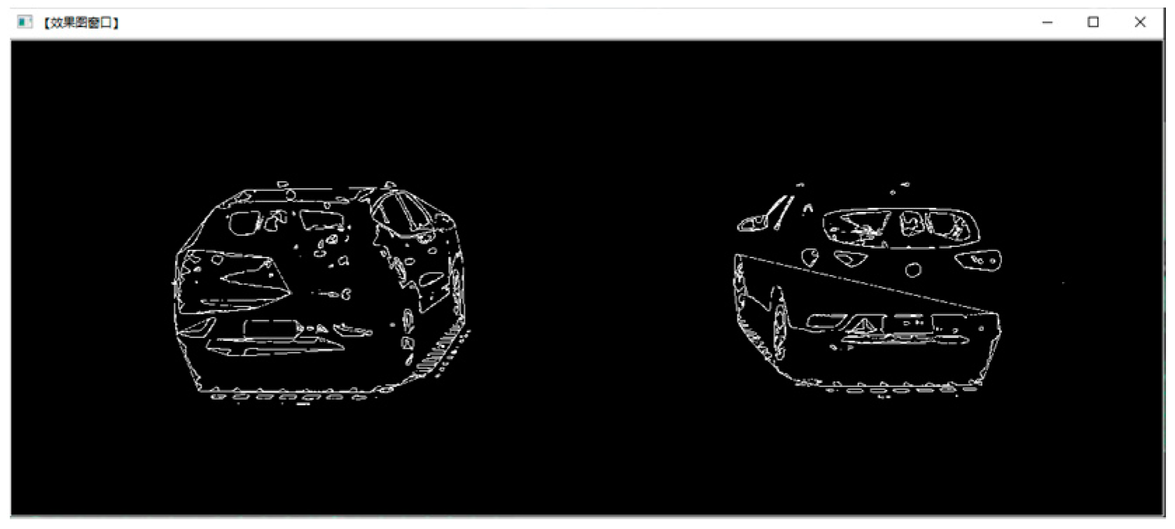
4.1. Contour Detection

Processing the image results in pixel gray values of similarity and discontinuity, which makes it easy for contour boundary detection [25,26]. The effects of this are shown in Figure 11 below.

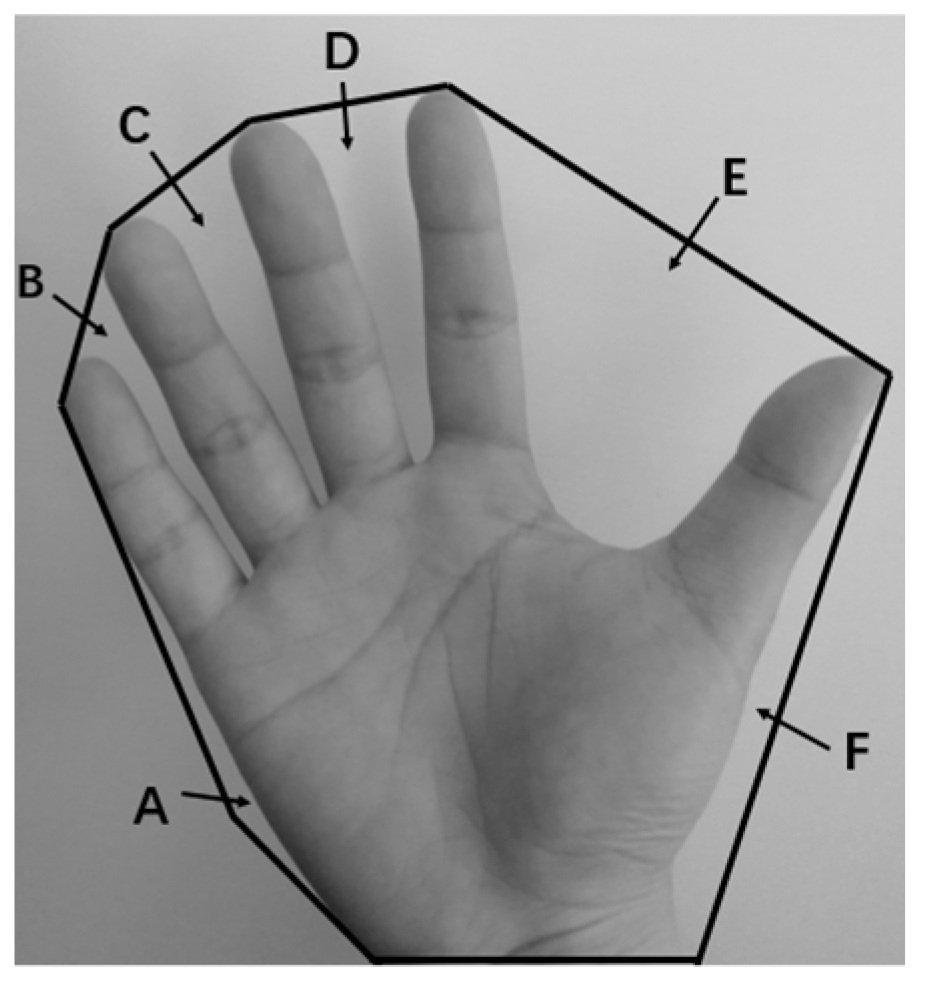
4.2. Convex Hull Detection

The convex hull is a concept in computational geometry or graphics, which may be defined as the smallest convex points containing the given points, which is the intersection of all convex points that contain the given points in the Euclidean plane or space. It can be imagined as a rubber band that just wraps all the points.

A useful method for understanding the shape contour of an object is to calculate the convex hull of the object and then calculate the convex defect [27]. The performance of many complex objects can be represented by this defect.

As shown in Figure 12, convex defects can be illustrated by human hands. The dark contour line is a convex hull around the hand. The regions (A-F) between the convex hull and the hand contour are convex defects.

4.3. Division of Obstacle Areas

Changes in the laser grids on the ground indicate that there is a potential obstacle on the ground, which results in different pixel gray values for the background and the obstacles.

The obstacles and the background are captured by the discontinuity of the boundary regions between them through the adjustments of the contour threshold of the ground laser grid area, segmentation of the ground laser grid area, the obstacle layer, and locating the coordinate region where the obstacle is located through the laser mesh deformation area, as shown in Figure 13.

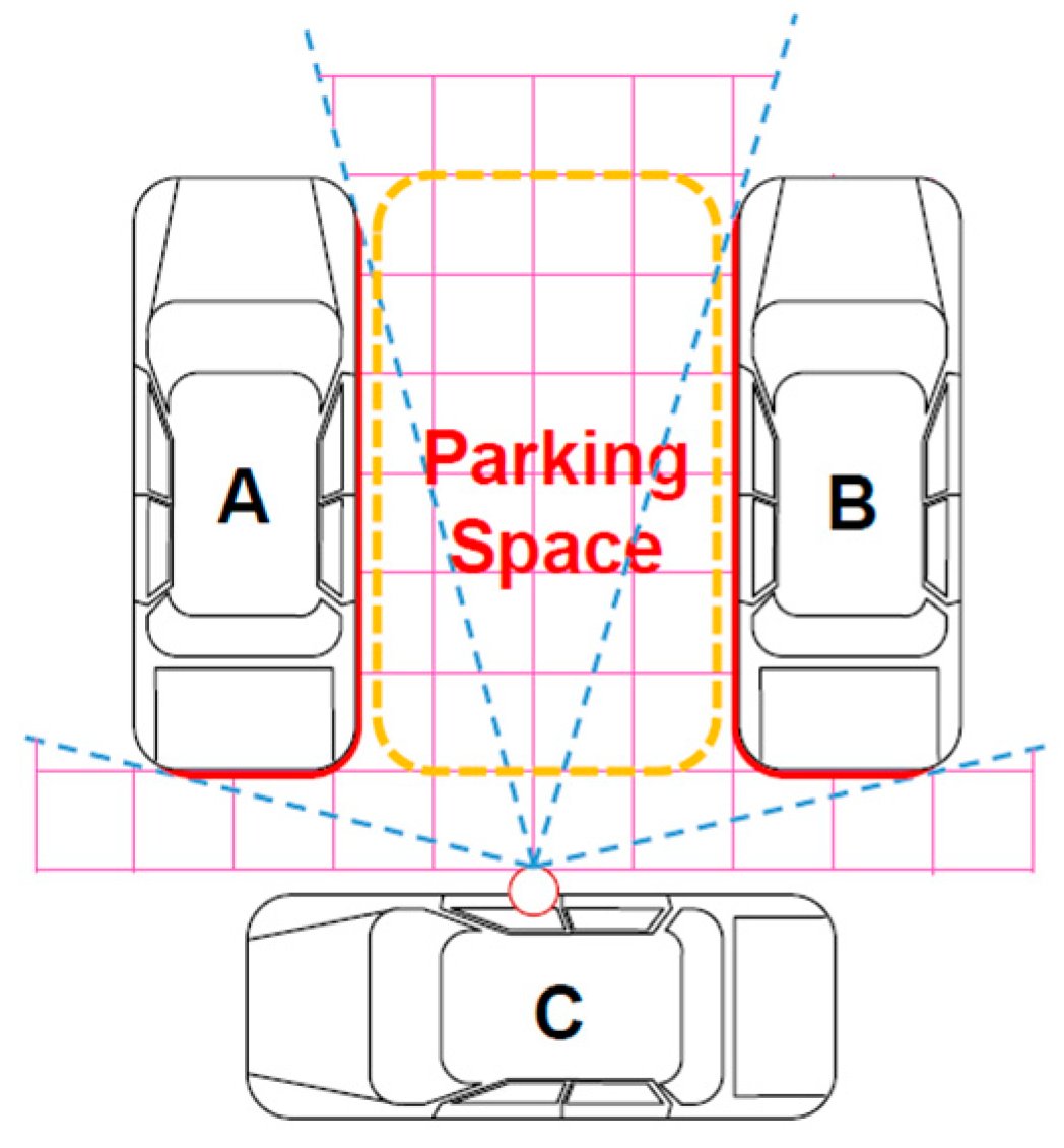
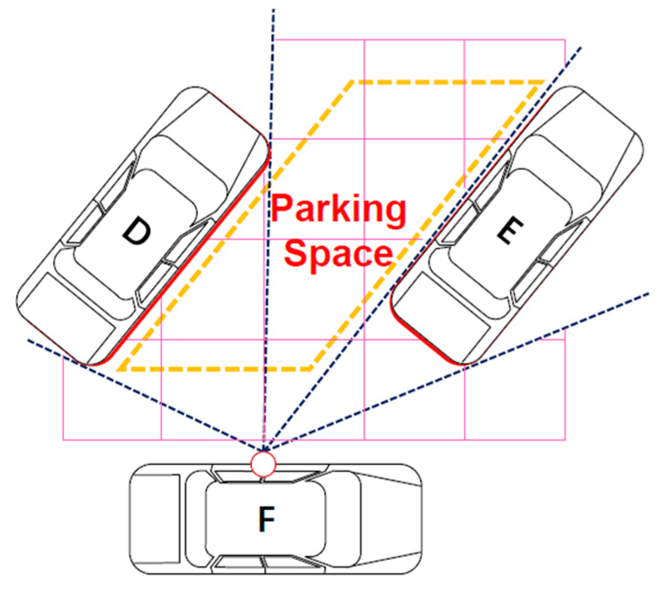
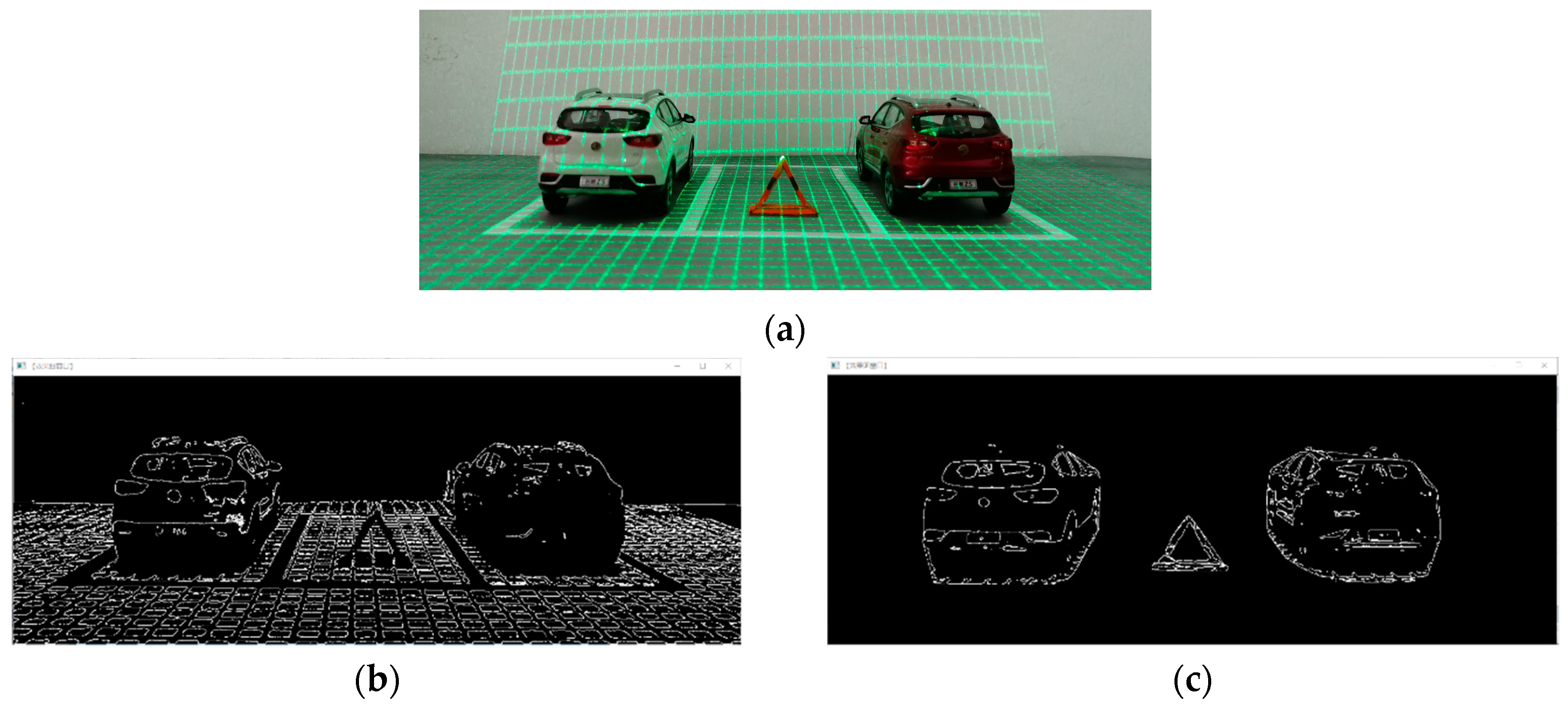
4.4. Parking Space Identification

The recognition of the parking space mainly involves the acquisition of the type of parking space and judging whether the identified parking space can meet the parking conditions. The types of parking spaces are shown in

Table 1. Different types of parking spaces.

Parking Modes	Parking Lines	Vehicles Around
Vertical parking	Standard parking lines	One side
Parallel parking	Only parking angles	Both sides
Oblique parking	No parking line	None

. We can classify them according to the parking modes, the existence of parking lines, and the existence of vehicles around. Because most research is mainly about parking spaces with parking lines and surrounding vehicles, this part only includes the situation without parking lines and vehicles on both sides. Because the parallel parking mode and the vertical parking mode are similar in terms of the identification methods, this part takes the latter as an example.

As shown in Figure 14 and Figure 15, the laser emitting devices are illuminated on the ground to present the shape of the checkerboard grid. We divide the region of vehicles and parking space by acquiring the contours of vehicles when processing the captured image of the parking space. According to the contours of the A, B, D, and E cars, we can judge the posture of the vehicle body, thereby we can acquire the type of paring space, such as a vertical parking space and an oblique parking space. The laser grid area between two cars’ contours can be considered as the area of the parking space. If there are no obstacles in this area, then the parking space can be considered as valid.

5. Experiments

The experiment was made up of the hardware parts, as shown in Figure 16, and the software parts. The hardware consisted of a grid laser emitter with a 51 × 51 laser grid on the ground and a camera, while the software part consisted of image processing and obstacle detection by the on-board computer. The implementation of the software part was done using C++ with Visual Studio 2017 as the development environment using OpenCV library Version 3.4.4 for image processing and obstacle detection.

In order to verify the effectiveness of the proposed method for identifying parking spaces and obstacles based on vision sensors and laser devices, various obstacles and scenes encountered in real-life parking environments were simulated and tested by the experimental platform in Figure 16. The laser transmitter and the camera mounted on the vehicle were simulated on the experimental platform, then the laser emitter and camera were adjusted to the appropriate angle so that the laser transmitter was evenly distributed on the ground to render a checkerboard laser grid effect while the parking space scenes were simulated through the model cars. As shown in Figure 17 and Figure 18, after collecting the images of the simulated scenes, codes were written that called the function of the OpenCV library to preprocess the image and detect the contour and convex hull. In the process of image processing, only the laser grid on the ground was used as the region of interest, and the image threshold was changed to reveal the contour of the laser mesh. The effect diagram is shown in Figure 19.

The gray value of the background in the scenes, such as the wall and the parking line, was different from the gray value of the ground laser line; therefore, it would be filtered out. The deformation region of the laser grid on the ground was then taken as the region of interest, by adjusting the threshold of the image, revealing the contours of obstacles, as shown in Figure 20.

As shown in Figure 21 and Figure 22, when there were obstacles and parking locks in the parking space, the contours could be adjusted by taking the laser grid and the deformation region of the laser grid on the ground as the region of interest, respectively. It showed the area where the obstacle was located and the size of the obstacles, making it convenient for the identification of the parking space area and the judgment of the adequate parking space.

For the classification and experiment of different types of obstacles that may exist in the parking space in the actual parking environment, an experiment with regular obstacles, potholes, and obstacles with a similar color to the background was carried out, as shown in Figure 23 and Figure 24, respectively. Nevertheless, when the color of the obstacle was similar to the background, it was challenging to identify the outline of the obstacle area through image processing alone. However, when we experimented with the proposed method of combining the camera vision and the laser grid, the area and contour of the obstacles could easily be obtained even when the obstacle was similar to the color of the background, as indicated in Figure 25 and Figure 26.

Table 2. The results of recognizing the contours of different types of obstacles in parking spaces.

Model Types	Regular	Irregular	Similar to the Ground Color
Vehicle	$\frac{63}{64}=98.4\%$	-	-
Wall/Pillar	$\frac{20}{20}=100\%$	-	$\frac{20}{20}=100\%$
Parking lock	$\frac{43}{46}=93.5\%$	-	-
Stone	$\frac{37}{38}=97.4\%$	$\frac{37}{38}=97.4\%$	$\frac{36}{38}=94.7\%$
Pothole	$\frac{38}{40}=95.0\%$	$\frac{39}{40}=97.5\%$	$\frac{38}{40}=95.0\%$

shows the test results of different types of obstacles’ recognition accuracy.

6. Conclusions and Future Research

In order to overcome the problems existing in current automatic parking schemes, ultrasonic radar and cameras are not efficient in identifying adequate parking spaces and cannot identify obstacles in parking paths or parking spaces. This paper presents a method to identify parking spaces and obstacles based on visual sensor and laser device recognition methods. This method only needs to install the laser transmitter on the body of the car. The changing images of the laser mesh are captured by the camera, and then, the changing area of the laser grids can be identified by image processing technology to realize the identification of parking spaces and obstacles. This method is expected to become a practical solution. The experimental results showed that this method could effectively identify obstacles and parking spaces.

For future research, more obstacle samples will be taken into consideration. The methods to deal with the automatic classification of obstacles need to be found. In addition, experiments for identifying the parking space and acquiring the size of the parking space, as well as obstacles still need to be conducted. Overall, this research provided a new solution to recognize obstacles for automatic parking. The future research will also greatly help the development of this technology.

References

1. Song, Y.; Liao, C. Analysis and review of state-of-the-art automatic parking assist system. In Proceedings of the 2016 IEEE International Conference on Vehicular Electronics and Safety (ICVES), Beijing, China, 10–12 July 2016; pp. 1–6. [Google Scholar]
2. Bibi, N.; Majid, M.N.; Dawood, H.; Guo, P. Automatic parking space detection system. In Proceedings of the 2017 2nd International Conference on Multimedia and Image Processing (ICMIP), Wuhan, China, 17–19 March 2017; pp. 11–15. [Google Scholar]
3. Prophet, R.; Hoffmann, M.; Vossiek, M.; Li, G.; Sturm, C. Parking space detection from a radar based target list. In Proceedings of the 2017 IEEE MTT-S International Conference on Microwaves for Intelligent Mobility (ICMIM), Nagoya, Japan, 19–21 March 2017; pp. 91–94. [Google Scholar]
4. Luo, Q.; Saigal, R.; Hampshire, R.; Wu, X. A Statistical Method for Parking Spaces Occupancy Detection via Automotive Radars. In Proceedings of the 2017 IEEE 85th Vehicular Technology Conference (VTC Spring), Sydney, NSW, Australia, 4–7 June 2017; pp. 1–5. [Google Scholar]
5. Ma, S.; Jiang, H.; Han, M.; Xie, J.; Li, C. Research on automatic parking systems based on parking scene recognition. IEEE Access 2017, 5, 21901–21917. [Google Scholar] [CrossRef]
6. Suhr, J.K.; Jung, H.G.J.S. A universal vacant parking slot recognition system using sensors mounted on off-the-shelf vehicles. Sensors 2018, 18, 1213. [Google Scholar] [CrossRef] [PubMed] [Green Version]
7. Chen, F. Research on Automatic Parking Technology Based on Machine Vision. Master’s Thesis, Electronic Science and Technology Univ., Chengdu, China, 2016. [Google Scholar]
8. Jung, H.G.; Kim, D.S.; Yoon, P.J.; Kim, J. Light stripe projection based parking space detection for intelligent parking assist system. In Proceedings of the 2007 IEEE Intelligent Vehicles Symposium, Istanbul, Turkey, 13–15 June 2007; pp. 962–968. [Google Scholar]
9. Catapang, A.N.; Ramos, M. Obstacle detection using a 2D LIDAR system for an Autonomous Vehicle. In Proceedings of the 2016 6th IEEE International Conference on Control System, Computing and Engineering (ICCSCE), Batu Ferringhi, Malaysia, 25–27 November 2016; pp. 441–445. [Google Scholar]
10. Shi, X.L. Research of Automatic Parking System Based on Laser Radar. Master’s Thesis, Shanghai Jiao Tong Univ., Shanghai, China, 2010. [Google Scholar]
11. Lee, B.; Wei, Y.; Guo, I.Y. Automatic parking of self-driving car based on lidar. Remote Sens. Spat. Inf. Sci. 2017, 42, 241–246. [Google Scholar] [CrossRef] [Green Version]
12. Jiang, H.B.; Shen, Z.N. Intelligent identification of automatic parking system based on information fusion. J. Mech. Eng. 2017, 53, 125–133. [Google Scholar] [CrossRef]
13. Suhr, J.; Jung, H.J.E.L. Sensor fusion-based precise obstacle localisation for automatic parking systems. Electron. Lett. 2018, 54, 445–447. [Google Scholar] [CrossRef] [Green Version]
14. Ibisch, A.; Stümper, S.; Altinger, H.; Neuhausen, M.; Tschentscher, M.; Schlipsing, M.; Salinen, J.; Knoll, A. Towards autonomous driving in a parking garage: Vehicle localization and tracking using environment-embedded lidar sensors. In Proceedings of the 2013 IEEE Intelligent Vehicles Symposium (IV), Gold Coast, QLD, Australia, 23–26 June 2013; pp. 829–834. [Google Scholar]
15. Park, J.; Lee, J.H.; Son, S.H. A survey of obstacle detection using vision sensor for autonomous vehicles. In Proceedings of the 2016 IEEE 22nd International Conference on Embedded and Real-Time Computing Systems and Applications (RTCSA), Daegu, Korea, 17–19 August 2016; p. 264. [Google Scholar]
16. Ho, T.; Budagavi, M. Dual-fisheye lens stitching for 360-degree imaging. In Proceedings of the 2017 IEEE International Conference on Acoustics, Speech and Signal Processing (ICASSP), New Orleans, LA, USA, 5–9 March 2017; pp. 2172–2176. [Google Scholar]
17. Zhang, Z. Flexible Camera Calibration by Viewing a Plane from Unknown Orientations. In Proceedings of the 7th IEEE International Conference on Computer Vision (ICCV’99), Kerkyra, Greece, 20–27 September 1999; pp. 666–673. [Google Scholar]
18. Zhang, J.; Wang, D.; Ma, L. The self-calibration technology of camera intrinsic parameters calibration methods. J. Imaging Sci. Photochem. 2016, 34, 15–22. [Google Scholar]
19. Sun, Q.; Wang, X.; Xu, J.; Wang, L.; Zhang, H.; Yu, J.; Su, T.; Zhang, X.J.O. Camera self-calibration with lens distortion. Opt. In. J. Light Electron Opt. 2016, 127, 4506–4513. [Google Scholar] [CrossRef]
20. Geiger, A.; Moosmann, F.; Car, Ö.; Schuster, B. Automatic camera and range sensor calibration using a single shot. In Proceedings of the 2012 IEEE International Conference on Robotics and Automation, Saint Paul, MN, USA, 14–18 May 2012; pp. 3936–3943. [Google Scholar]
21. Zhang, X.; Wang, X. Novel survey on the color-image graying algorithm. In Proceedings of the 2016 IEEE International Conference on Computer and Information Technology (CIT), Nadi, Fiji, 8–10 December 2016; pp. 750–753. [Google Scholar]
22. Gupta, V.; Gandhi, D.K.; Yadav, P. Removal of fixed value impulse noise using improved mean filter for image enhancement. In Proceedings of the 2013 Nirma University International Conference on Engineering (NUiCONE), Ahmedabad, India, 28–30 November 2013; pp. 1–5. [Google Scholar]
23. Huang, S.; Cheng, F.; Chiu, Y. Efficient contrast enhancement using adaptive gamma correction with weighting distribution. IEEE Trans. Image Process. 2012, 22, 1032–1041. [Google Scholar] [CrossRef]
24. Mahashwari, T.; Asthana, A. Image enhancement using fuzzy technique. Int. J. Res. Eng. Sci. Technol. 2013, 2, 1–4. [Google Scholar]
25. Xie, S.; Tu, Z. Holistically-nested edge detection. In Proceedings of the IEEE International Conference on Computer Vision, Santiago, Chile, 11–18 December 2015; pp. 1395–1403. [Google Scholar]
26. Gurav, R.M.; Kadbe, P.K. Real time finger tracking and contour detection for gesture recognition using OpenCV. In Proceedings of the 2015 International Conference on Industrial Instrumentation and Control (ICIC), Pune, India, 28–30 May 2015; pp. 974–977. [Google Scholar]
27. Singh, N.; Arya, R.; Agrawal, R. A convex hull approach in conjunction with Gaussian mixture model for salient object detection. Digit. Signal Process. 2016, 55, 22–31. [Google Scholar] [CrossRef]
Figure 1. System construction.
Applsci 10 02582 g001
Figure 2. System schematic.
Applsci 10 02582 g002
Figure 3. Algorithm flow.
Applsci 10 02582 g003
Figure 4. Rendering of the laser grid on the ground.
Applsci 10 02582 g004
Figure 5. The ideal laser grid image.
Applsci 10 02582 g005
Figure 6. The actual laser grid image.
Applsci 10 02582 g006
Figure 7. Obstacle area testing.
Applsci 10 02582 g007
Figure 8. The conversion of a pixel by the mean filter.
Applsci 10 02582 g008
Figure 9. Gamma transformation curve.
Applsci 10 02582 g009
Figure 10. (a) The original image; (b) gamma transform corrected image.
Applsci 10 02582 g010
Figure 11. The contour of images.
Applsci 10 02582 g011
Figure 12. The convex hull and convex defects.
Applsci 10 02582 g012
Figure 13. Division of obstacle areas. (a) The area of the obstacle; (b) the area of the ground.
Applsci 10 02582 g013
Figure 14. Vertical parking mode.
Applsci 10 02582 g014
Figure 15. Oblique parking mode.
Applsci 10 02582 g015
Figure 16. Experiment platform. (a) front view; (b) side view.
Applsci 10 02582 g016
Figure 17. The image of the parking space.
Applsci 10 02582 g017
Figure 18. Gamma-enhanced image.
Applsci 10 02582 g018
Figure 19. The contour of the laser grid.
Applsci 10 02582 g019
Figure 20. The contour of the cars.
Applsci 10 02582 g020
Figure 21. The obstacle exists in the parking space. (a) The image of the parking space; (b) the contour of the laser grid; (c) the contour of cars and the obstacle.
Applsci 10 02582 g021
Figure 22. A parking lock exist in the parking space. (a) The image of the parking space; (b) the contour of the laser grid; (c) the contour of the cars and the parking lock.
Applsci 10 02582 g022
Figure 23. Obstacle and pothole. (a) The regular block obstacle; (b) the contour of the ground; (c) the contour of the block obstacle; (d) the regular pothole; (e) the contour of the ground; (f) the contour of the regular pothole.
Applsci 10 02582 g023
Figure 24. (a) The irregular obstacle that was similar in color to the background; (b) the irregular contour of the obstacle is very vague.
Applsci 10 02582 g024
Figure 25. The irregular obstacle that was similar in color to the background. (a) The irregular obstacle (b) the contour of the ground; (c) the contour of the irregular obstacle.
Applsci 10 02582 g025
Figure 26. The irregular pothole that was similar in color to the background. (a) The irregular pothole (b) the contour of the ground; (c) the contour of the irregular pothole.
Applsci 10 02582 g026