Research on Lane Detection Based on Global Search of Dynamic Region of Interest (DROI)

Abstract

A novel lane detection approach, based on the dynamic region of interest (DROI) selection in the horizontal and vertical safety vision, is proposed to improve the accuracy of lane detection in this paper. The curvature of each point on the edge of the road and the maximum safe distance, which are solved by the lane line equation and vehicle speed data of the previous frame, are used to accurately select the DROI at the current moment. Next, the global search of DROI is applied to identify the lane line feature points. Subsequently, the discontinuous points are processed by interpolation. To fulfill fast and accurate matching of lane feature points and mathematical equations, the lane line is fitted in the polar coordinate equation. The proposed approach was verified by the Caltech database, under the premise of ensuring real-time performance. The accuracy rate was 99.21% which is superior to other mainstream methods described in the literature. Furthermore, to test the robustness of the proposed method, it was tested in 5683 frames of complicated real road pictures, and the positive detection rate was 99.07%.

1. Introduction

In recent years, advanced driver assistance systems (ADAS) and autonomous driving are becoming more and more important to reducing traffic accidents. As a key technology for intelligent vehicles, lane detection has attracted widespread attention from plenty of institutes and automobile technology companies [1]. Among the research, vision-based lane detection has always been a hot topic in the field of lane line detection. For example, in these studies, the selection of the region of interest (ROI) has been widely used to limit the range of lane detection because it can efficiently reduce the level of redundant data to improve the real-time capabilities and accuracy. In [2], one quarter of entire image, i.e., near the bottom of the image, was selected as the ROI; however, the hood and front windshield of the car can cause false edges, which would affect subsequent lane line detection. In order to improve the accuracy capabilities, the vanishing point of the lane line, indicating the point at which two lane lines cross in the distance, was treated as the upper boundary of the ROI [3,4,5]. Then, Hai [6] proposed setting two thirds of the region below the vanishing point as the ROI. Although the calculation amount of this method is less than that of the method with the vanishing point as the upper boundary, this method still cannot effectively extract the ROI following a safe distance from the front field of view. Similarly, to improve detection performance, the ROI was separated into two parts and the piecewise linear stretch function was used to enhance the pixels of images in the region; however, the boundary was difficult to select [7]. Furthermore, in [8], to improve the accuracy of lane detection, the static ROI was divided into four subareas, i.e., the left and right lane lines in the near and far fields of view, but it was subject to interference by false edges such as disturbances in the road or obstacles on either side. Gaikwad [9] proposed the use of the first frame of the lane detection images to initialize the ROI; detection would then be performed according to the ROI; however, the accuracy of the approach needs to be improved.

When it comes to lane models, except for the widely applied mathematical models, (including the straight line, parabola, hyperbolic and line-parabola models), the three-dimensional traffic model was established by analyzing the lane space structure [10]. Because the straight line model cannot be used to fit the lane line in complicated environments, models such as parabola and hyperbola need to be utilized to match the lane line [11]. A simple parabola model [12,13,14] which combines the position of the lane line, the angle and the changed curvature, was presented, but this model cannot fit a transitional connection between a straight lane line and a curved lane line. In order to adapt to the constant transformation of lane lines, parabolic models need to be replaced by a higher order model [15]. An improved model, combining straight and curved lanes and geometric constraints, was proposed in which the second derivative of a quadratic curve was used as the basis to estimate the condition of the road [16]. Although this method enhances flexibility, it is still difficult to use it to search for the connection point between the straight line and the curve.

In view of the above works, a novel lane detection method based on the DROI is proposed in this paper; firstly, to fulfill the accurate selection of the ROI, the lane line equation and the vehicle speed of the last frame are utilized to solve the curvature of the points on the lane edge and the maximum safe distance. Then, the feature points of the lane line are detected using DROI global searching. Lastly, the lane line is fitted by the polar equation and the fitting effect is good.

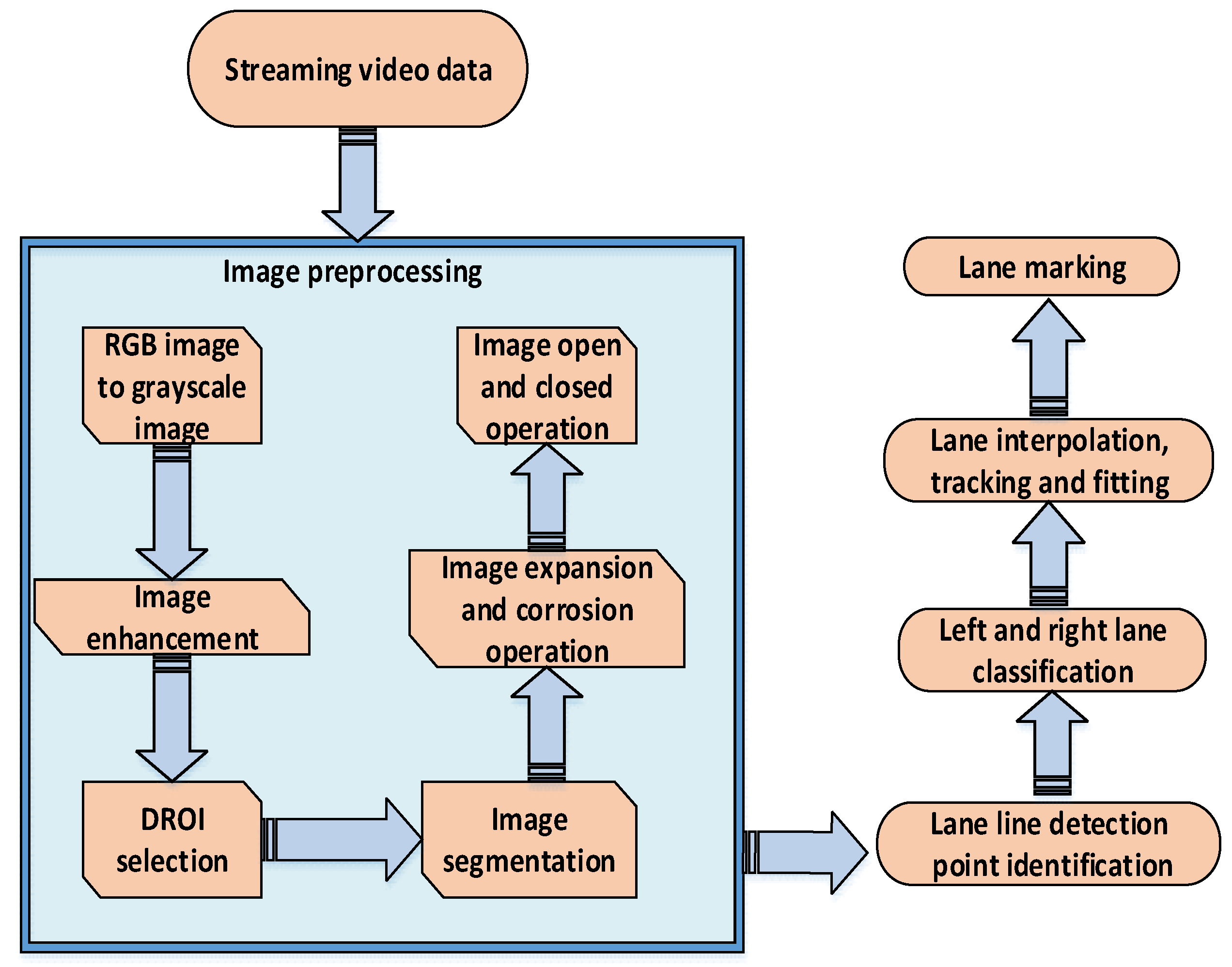
2. Image Preprocessing

Image preprocessing needs to be properly performed to successfully extract the lane line pixels in images and complete the lane line detection. First of all, image graying needs to be done to reduce the calculation load, because the original images contain too much miscellaneous or repetitive information. After the grayscale image is obtained, the distinction between lane line information and other interference is weakened. Therefore, in order to highlight the lane information in the image and reduce or remove the interference information, image enhancement processing needs to be carried out on the gray image. After obtaining the enhanced image with a clear difference between lane line and interference information, image segmentation on local OTSU (maximum between-cluster variance algorithm) needs to be used to extract the lane line information. Lastly, the inverse perspective transformation matrix transforms the image coordinates into real road coordinates.

2.1. Image Grayscale Processing

The data samples used in this paper come from the Udacity, Caltech and integrated databases, collected by a 1 mega camera (ds90ub913a) and an onsemi 1.0 mp ar0144rccb sensor. Because the format of the image data was RGB, the images were converted into grayscale images to reduce computing time. The grayscale is calculated by Equation (1) [17].

$$Gray=R\ast 0.3+G\ast 0.59+B\ast 0.11$$

(1)

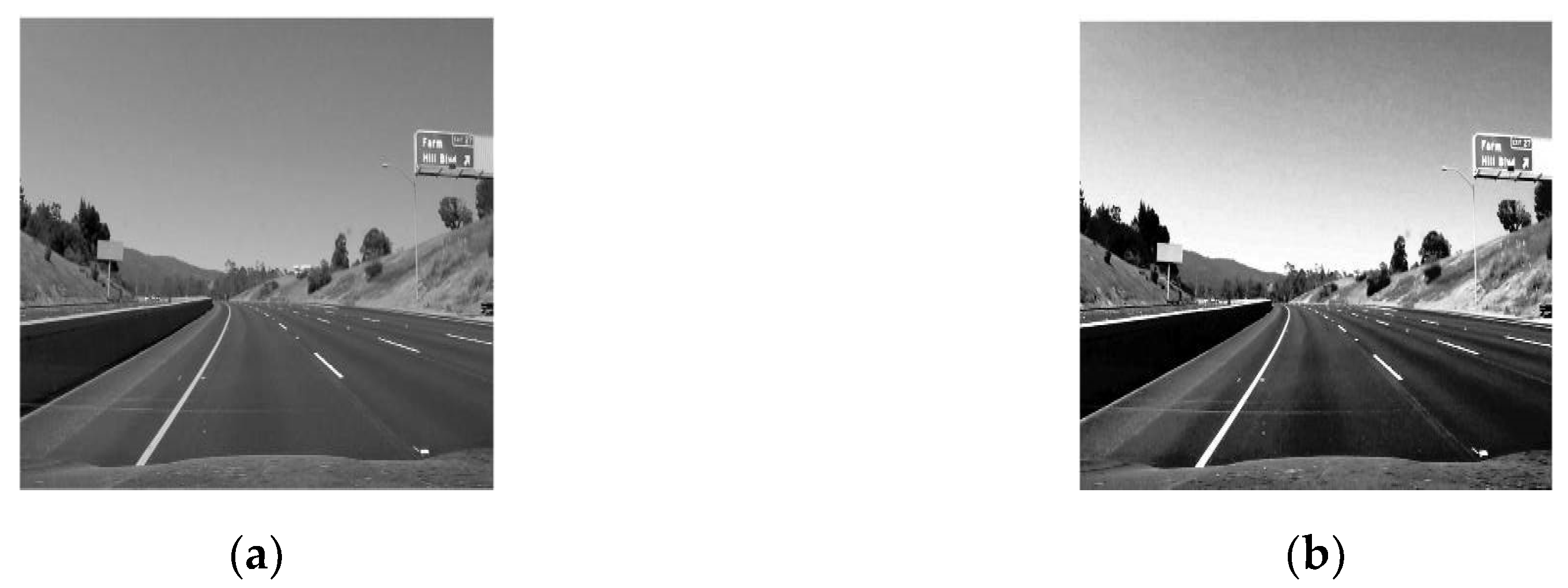
2.2. Image Enhancement Processing

To focus on the useful information and weaken or exclude interference information, the gray images need to be processed using image enhancement technology. Histogram equalization is applied to process the gray image, as it can increase the dynamic range of the pixels and lessen the computation load. After histogram equalization, the dynamic range of pixels becomes wider, and the difference between the lane line information and other interference information becomes more obvious. The effect of the histogram equalization is shown in the Figure 1.

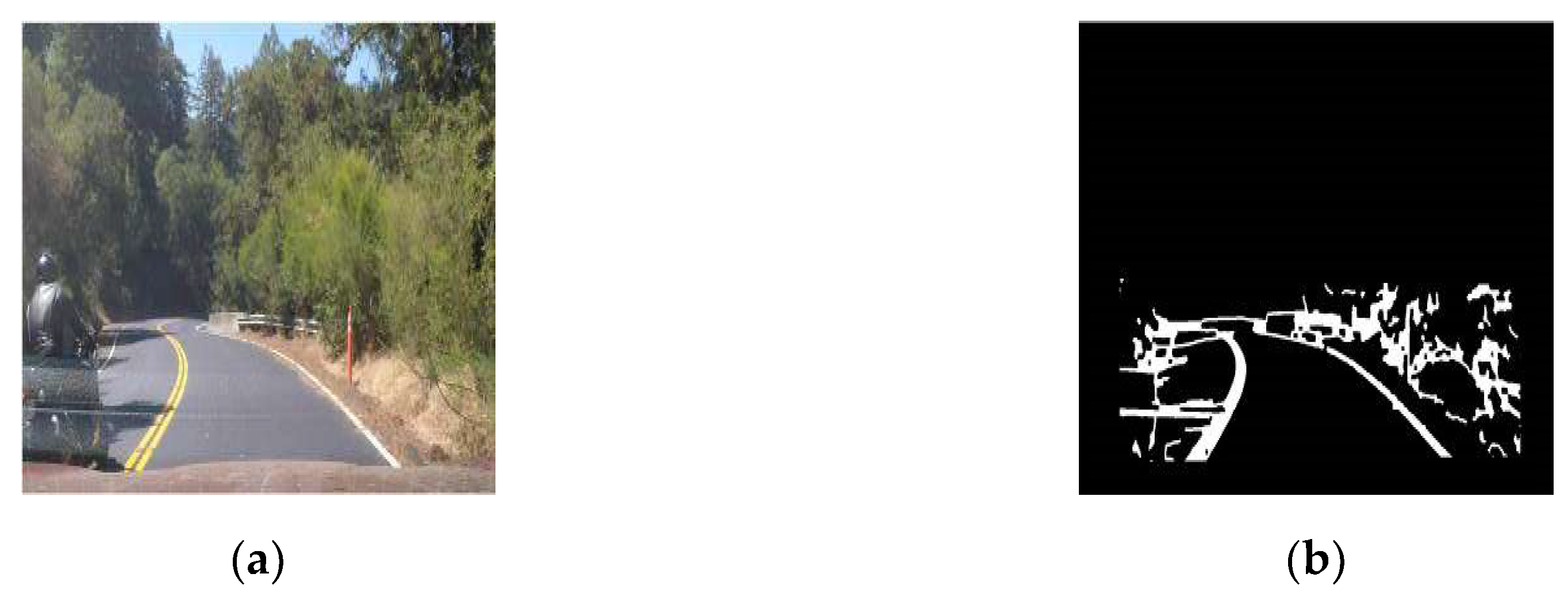
2.3. Image Segmentation on Local OTSU

In order to improve detection accuracy, the majority of the noise in the raw image should be processed in the background layer using image segmentation technology. The lane line can act as the objective layer. On the other hand, the method of the largest variance between classes is used to remove the interference information and achieve better segmentation of the road image. The variance between classes of the pixels [18], segmented by the image I(x, y), is computed by Equation (2).

$$\mathrm{g}={\omega }_0\ast {\omega }_1\ast {\left({\mu }_0-{\mu }_1\right)}^2$$

(2)

where ${\mu }_0$ and ${\mu }_1$ are the average gray of the segmented foreground and background, respectively, ${\omega }_1$ is the proportion of the background pixel in the raw image, and ${\omega }_0$ is the percentage of the pixel in the segmented image.

The traversal approach is used to search for the threshold value, which determines the largest variance between classes. In addition, local adaptive segmentation is applied to the road image. The image processing result is compared and shown in Figure 2.

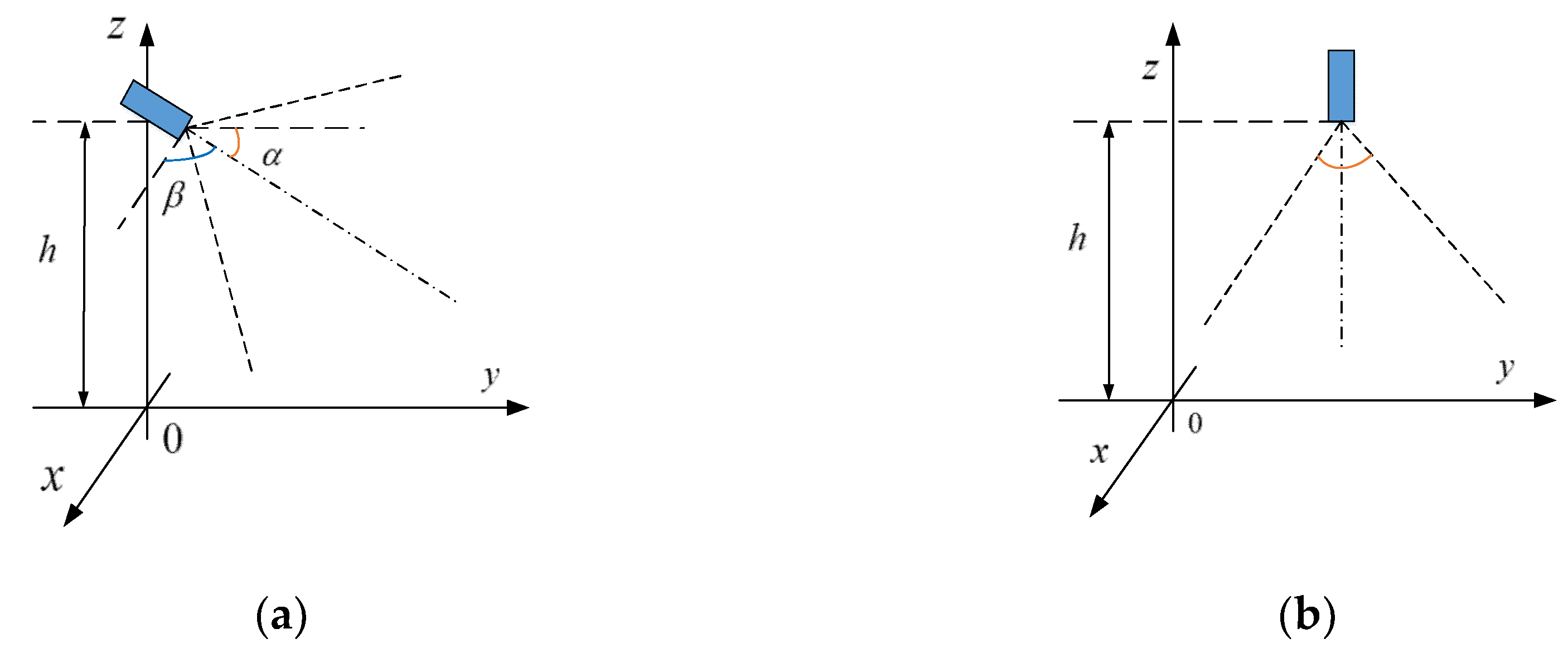
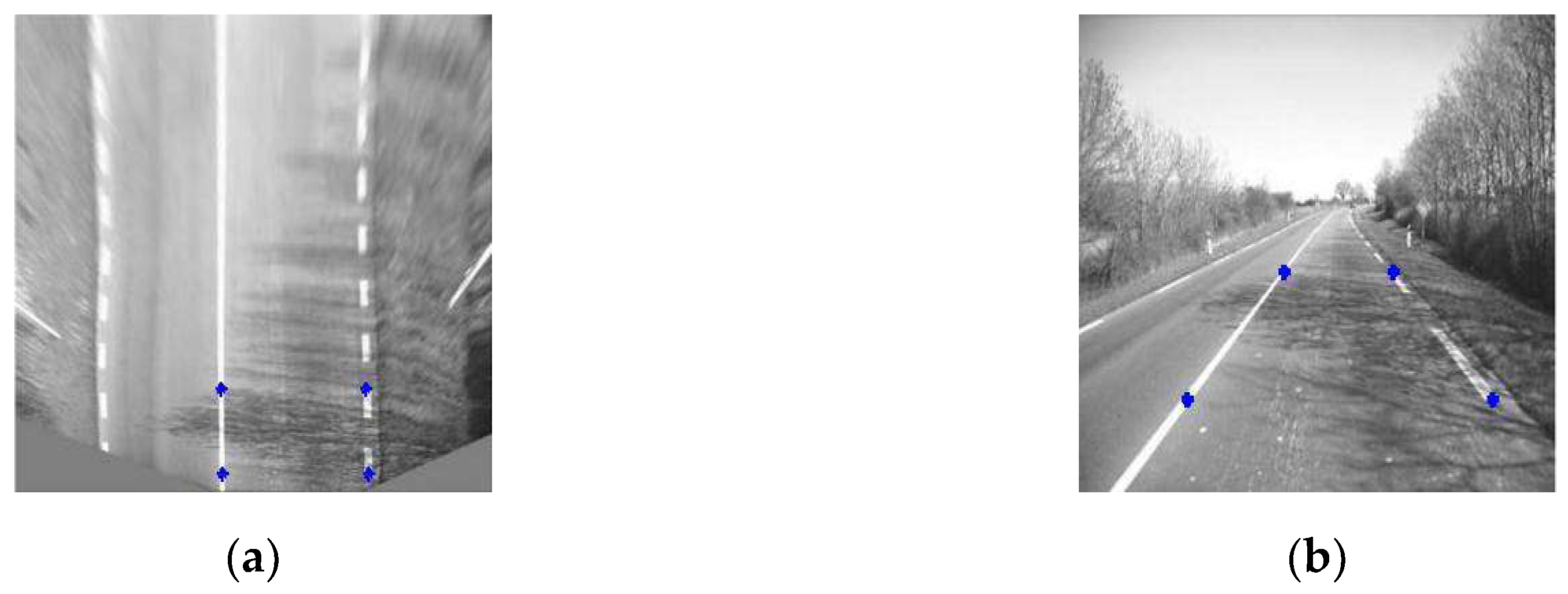
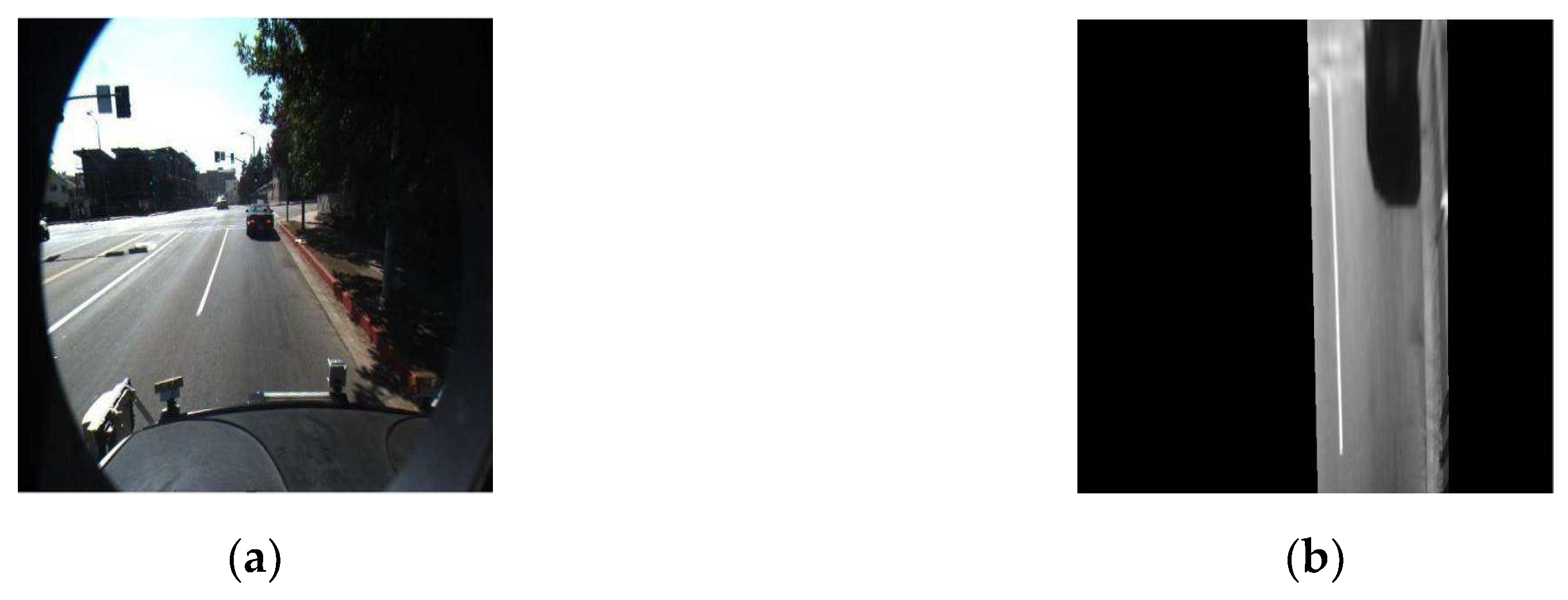
2.4. Inverse Perspective Transformation

Due to the perspective effect of the camera, the road image appears larger in the near vision and smaller in the far vision. A distorted road image is shown in Figure 1. To obtain the real road information, the road image needs to be processed by means of inverse perspective transformation [19]. After the transformation, the perspective effect of the camera is eliminated. The parallel lane line is shown in [20]. The perspective of the coordinate is shown in Figure 3.

Because affine transformation is based on the corresponding relationship of image coordinate transformation, the transformation from inverse perspective to aerial view can be performed [21]. The principle is as follows: the raw image is set as $U\left(u,v,w\right)$, and the transferred image is $I\left(x,y,1\right)$; the image coordinate, which is transferred by the transformation matrix, is $U^{\prime }\left(u^{\prime },v^{\prime },w^{\prime }\right)$. The alpha and beta angles represent the pitch and deviation angles of the on-board camera, respectively. The raw image coordinate system is the reference coordinate system, so w is set as 1. The expressions for x and y are as follows:

$$x=\frac{u^{\prime }}{w^{\prime }}$$

(3)

$$y=\frac{v^{\prime }}{w^{\prime }}$$

(4)

The matrix of transformation takes the following form:

$$\mathrm{T}=\left[\begin{array}{ccc}{t}_{11}& t_{12}& t_{13}\\ t_{21}& t_{22}& t_{23}\\ t_{31}& t_{32}& t_{33}\end{array}\right]$$

(5)

The aerial view transformation is expressed as:

$$U^{\prime }=TgU,$$

(6)

where $\mathrm{T}=\left[\begin{array}{cc}{t}_{11}& t_{12}\\ t_{21}& t_{22}\end{array}\right]$ denotes the linear transformation, the inverse transformation is $T_2={\left[\begin{array}{cc}{t}_{13}& t_{23}\end{array}\right]}^T$, and $T_3=\left[\begin{array}{cc}{t}_{31}& t_{32}\end{array}\right]$ represents the image transition.

Therefore, x and y can be calculated using Equations (7) and (8), respectively, with the value of $t_{33}$ being 1:

$$x=\frac{u^{\prime }}{w^{\prime }}=\frac{t_{11}u+t_{12}v+t_{13}}{t_{31}u+t_{32}v+t_{33}}$$

(7)

$$y=\frac{v^{\prime }}{w^{\prime }}=\frac{t_{21}u+t_{22}v+t_{23}}{t_{31}u+t_{32}v+t_{33}}$$

(8)

According to the equations, as long as the coordinates of four noncolinear points in the image are found, the transformation matrix T can be obtained. Then, each point coordinate in the aerial view, corresponding in the original image, can be solved using Equation (6). Figure 4 shows the aerial view obtained from the affine transformation; those that are marked in Figure 4 are the selected coordinate points.

3. Design of Dynamic Region of Interest (DROI) Based on Security Vision

3.1. Longitudinal Boundary Design of DROI Based on Safe Car Distance

In order to obtain a better ROI, in this paper, the concept of safety vision is introduced based on road traffic safety rules. Therefore, according to the adaptive security field of view, the DROI will be selected.

Generally, the field of vision comes from the front of the vehicle. In accordance with the focus of imitating human habits, this section restricts the longitudinal range of DROI to the safe distance.

The safety area of the front view refers to the distance when the car brakes in an emergency. If the speed of the vehicle is too high, the lane line vanishing point will be the longitudinal dynamic region of the interest boundary. Meanwhile, in order to ensure safety on roads with excessive curvatures, the speed must be less than the critical speed of rollover.

Since the lane line detection is aimed at matching the lane line equations in the pixel coordinate system, the image coordinate system must be converted into the geodetic coordinate system to find the longitudinal safe distance of vehicles. Firstly, the displacement ratio of the image coordinate system to the geodetic coordinate system is calibrated. Next, in the image coordinate system, the horizontal and longitudinal displacements of the lane are expressed in pixel coordinates. The minimum units are a row and a column. In the actual process, the displacement is described by m, so the difference between the two coordinate systems must be calibrated after the aerial view transformation [14]. The ratios of horizontal and vertical distances, between an image coordinate system and a geodetic coordinate system, are $a_x$ and $a_y$ respectively; they are given by:

$$a_x=\frac{l}{m},$$

(9)

$$a_y=\frac{s}{n},$$

(10)

where m denotes the value of the row in the pixel coordinates, 1 is the actual distance in the geodetic coordinates, n represents the value of the column, and s indicates the value of the realistic length in the geodetic coordinates.

The aggregation equations of the feature points in the left and right lane line image are given below.

$$y_l=f_l\left(x_l\right)$$

(11)

$$y_r=f_r\left(x_r\right)$$

(12)

The aggregation equations of the left and right lane line points represented in the geodetic coordinate are shown in Equation (13):

$$\{\begin{array}{c}{\widehat{x}}_l=x_l\times a_x=x_l\times \frac{l}{m}\\ {\widehat{y}}_l=y_l\times a_y=y_l\times \frac{s}{n}\end{array}\{\begin{array}{c}{\widehat{x}}_r=x_r\times a_x=x_r\times \frac{l}{m}\\ {\widehat{y}}_r=y_r\times a_y=y_r\times \frac{s}{n}\end{array}$$

(13)

The curvature equation in the rectangular coordinate system is as follows:

$$\rho =\frac{1}{r}=\frac{{\left(1+{y^{\prime }}^2\right)}^{\frac{3}{2}}}{\left|y^{″}\right|}$$

(14)

The radius of curvature of lane lines is calculated by the radius of curvature equation:

$$r=\frac{1}{\rho }$$

(15)

The slope at a certain point of the lane line is shown below:

$$y^{\prime }=tan\beta$$

(16)

$v_c$ can be calculated by the following inverse trig function:

$$v_c=v_{r}sin\beta ,$$

(17)

where $\beta$ is the inclination angle of the tangent line at each point under the track of the lane line, $v_c$ is the longitudinal speed of the lane line, and $v_r$ is the vehicle speed at the current frame.

The empirical formula between speed and brake distance is as follows [22]:

$$y_p=f\left(v_c\right)=\frac{1}{30\times 0.348}{v}_c{}^2+3.675v_c$$

(18)

Now, according to the relationship between the actual displacement and the image pixel, the boundary of the left and right lane lines in the image can be determined.

3.2. Lateral Boundary Design of DROI Based on Road Curvature

In order to reduce computation in the lateral vision and improve detection performance, the lateral ROI constraint, based on road curvature, is proposed. If the curvature of the road is too large, according to the road extension direction, the left and right lateral boundaries will be set. For example, considering a left-hand bend, the ROI boundary on the left is large while that on the right remains within the basic range. Similarly, if a car drives in a straight line, the left and right ROI boundaries remain within the basic safety range. The flow chart of the horizontal ROI constraint is shown in Figure 5.

To obtain the road curvature, firstly, according to the road extension direction, the track equation of the lane line is obtained. Next, the curvature radius at each point of the road can be solved through the track equation of the lane line. Because the time difference between the two adjacent frames of the road image is very small, even if the car is driving at a high speed of 120 km/h, the displacement difference between the two adjacent frames is less than 1.3 m. Therefore, the boundary of the ROI, which is obtained from the lane line track of the above frame, is used as the ROI of the next frame.

The curve equation of lane line trajectory is as follows:

$$y_l=f_{\mathrm{cv}}\left(x_l\right)$$

(19)

The lateral velocity of the car at each point in the lane line curve can be obtained using the following equation:

$$v_x=v_{r}cos\beta$$

(20)

Because the original lane line image is transformed by the aerial view, the generated aerial view is approximately equally spaced in the horizontal and vertical directions. Therefore, the horizontal pixel size of the image has a certain proportional relationship with the actual horizontal distance; its longitudinal distance also has a corresponding proportional relationship.

In the geodetic coordinate system, the distance between the left and right lane lines is $\mathsf{\lambda }=3.75\mathrm{m}$. In the image coordinate system, $g_l\left(u_i,v_j\right)$ and $g_r\left(u_{i+a},v_j\right)$ are selected at the same height of the left and right lane lines, respectively, and the lateral displacement between these two points is the distance between the left and right lane lines in the image. The lateral displacement is as follows:

$$B=u_{i+a}-u_i$$

(21)

The ratio of the actual distance to the rows in a horizontal pixel is represented by $\mu$.

$$u=\frac{B}{\mathsf{\lambda }}$$

(22)

According to the rules of safe driving, when the lane line is straight, the basic lateral safety constraint is $0.875/u$. Eventually, the lateral boundary can be obtained by the relationship between braking distance and speed, as given by Equation (18).

In the actual lane line detection process, in order to avoid excessive calculation errors in the lateral boundary caused by pixel differences, lane lines are detected in the aerial view in this paper as shown in Figure 6. At the same time, the ROI, which is determined by the lane line in the current frame, is used in the aerial view in the next frame.

4. Lane Detection and Tracking

In order to better achieve lane line detection, on the basis of image preprocessing of the original image, a lane line detection algorithm is used to detect the lane line contour. Meanwhile, the detected lane line data is divided into left and right lane line data sets, and the mathematical equation of lane line is established by interpolation, prediction and fitting. The detailed lane line flow is shown in Figure 7.

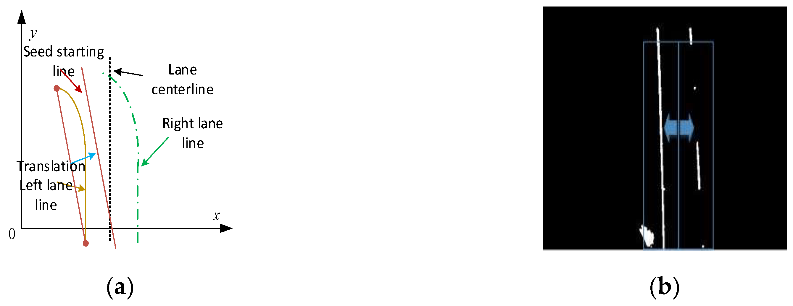
4.1. Detection Principle of the DROI Global Research and Starting Point Design

Considering the complex lane environment, the noise on the actual road, as well as the absence and discontinuity of lane lines, a global search method based on DROI is proposed to identify lane line feature points. In this section, the seed function of pixel recognition is employed to conduct a global search for DROI and realize the recognition of lane line feature points. After a series of preprocessing, such as graying, image enhancement and image segmentation, the binary lane line image matrix is obtained.

In the image matrix, as shown in Figure 8b, the gray value of the lane line is 1, and the other parts are 0. The converted aerial view is shown in Figure 8a. The left and right lane lines are roughly distributed on both sides for lane line, so the starting point of the search can be set from the bottom. As shown in Figure 8a, the width of lane lines is about 10 pixels in the image. Because the lane lines are worn, they are not standard rectangles, and some edges are jagged.

Furthermore, in order to fulfill a more efficient global search of DROI, firstly, the principle of DROI global is established. Next, a tilt line is set as the starting point of each line search. If the straight line of all points can meet separate left and right lane lines and the tilt does not have the intersection point with the lane line in the field of vision scope, this line satisfies the conditions. Then, in this section, the direction of the lane line in the previous frame is used as the tilt direction of the starting line, and the specific line is shifted to the right by the halves of the lane line width when it is determined by the lowest and highest points of the left lane line in the previous frame. Lastly, the equation used to search for the starting line can be obtained according to the two-point method and the image translation rules. The specific search starting line is shown in Figure 9 and the search process is shown in

Table 1. Basic rule of the global search of dynamic region of interest.

The Principles of the DROI Global Search

Set the search seed function $H\left(x,y\right)$ Start to search from the bottom, and then stop the search at the ROI edge. Begin to search for the next line when the ROI edge is searched, and search each line only once. The next line should start to be searched when it reaches the boundary without searching the feature point. The inside edge of lane lines acts as the lane lines in the search results, which is conducive to driving safety, although it reduces the range of lane lines. The lane line search boundary should be set because there is no lane line in the area of the imaginary line.

According to the DROI global search principle, the seed function is set as $H\left(x,y\right)$ [21], and $Z\left(x,y\right)$ refers to the part of image where the filter $H\left(x,y\right)$ is applied.

Therefore, the judging function is expressed as follows:

$$\sigma \left(x,y\right)=Z\left(x,y\right)\times H\left(x,y\right)$$

(23)

In order to judge whether the point is the lane line or not, if the judging function satisfies $\sigma \left(x_i,y_i\right)\ge \mathsf{\lambda }$, the point can be identified as the point on the lane line [23]. If the threshold requirement is not met, the search should be continued before reaching the ROI boundary. Since the image function is a matrix, the seed can be set as a template of structural elements to carry out dot product operation on the image matrix.

The template of the seed function is as follows:

$$seed=\left[\begin{array}{ccc}{s}_{11}& s_{12}& s_{13}\\ s_{21}& s_{22}& s_{23}\\ s_{31}& s_{32}& s_{33}\end{array}\right],$$

(24)

where $s_{ij}$ is the element in the seed template, which can be selected according to the effect of the binary image. $s_{ij}$ is set to:

$$s_{ij}=1\left(i=1,2,3\dots \dots ,j=1,2,3\dots \right),$$

(25)

In addition, threshold λ is set as 9 in this paper. The seed function is calculated with the original road image to obtain the value and judge the lane line position. Then, the data of the lane line feature point is determined.

4.2. Special Point Analysis of Lane Line Detection

4.2.1. ROI Search Based on the Previous Image

The difference between the two adjacent frames is not small, but it is related to the speed of the vehicle. To improve the real-time capability of lane line detection, the search scope of the next frame can be set based on the last search. Therefore, if the lateral velocity of the vehicle is low, the scope of the DROI search is smaller than the previous area. Additionally, to avoid incorrect detection and misdetection of lane lines due to lessening the range of search, the on and off conditions of the local search should also be set simultaneously.

4.2.2. Lane line estimation based on another lane line

Some information from the raw image will be lost due to gray processing and the aerial view transformation. During image preprocessing, incomplete and worn lane lines can also be eliminated when some noise is removed. Thus, the lane lines will not be detected. In order to avoid this, the completed lane line can be utilized to estimate another lane line position. Concrete images are shown in Figure 10.

4.3. Interpolation of Lane Line Discontinuities

Due to the existence of dotted lines and worn lane lines, lane line detection cannot be carried out effectively. Therefore, in this paper, the missing points between line segments are filled by linear interpolation [24].

The first-order interpolation is as follows:

$$\mathrm{y}=\frac{x_1-x}{x_1-x_0}·y_0+\frac{x-x_0}{x_1-x_0}·y_1$$

(26)

The quadratic interpolation is given by:

$$\mathrm{y}=\frac{\left(x-x_1\right)\left(x-x_2\right)}{\left(x_0-x_1\right)\left(x_0-x_2\right)}·y_0+\frac{\left(x-x_0\right)\left(x-x_2\right)}{(x_1-x_0)\left(x_1-x_2\right)}·y_1+\frac{\left(x-x_0\right)\left(x-x_1\right)}{(x_2-x_0)\left(x_2-x_1\right)}·y_2,$$

(27)

For generally straight lanes or lanes with small curvature, first-order interpolation can supplement the missing data points. For roads with large curvatures, the quadratic interpolation method can better supplement the data of the missing points.

4.4. Feature Point Tracking of the Lane Line

In the process of lane line detection, due to stains on the road and occlusion from other vehicles, lane line absence will occur frequently, i.e., the lane line cannot be seen visually in a single frame. In such cases, lane line prediction and tracking are essential. Owing to the small computation load, the grey prediction method has good performance and does not need a large amount of original data for sample support, making it very suitable for lane line prediction [25].

To efficiently achieve lane line prediction and tracking, firstly, the lane line data is transformed into one-dimensional data, which takes the form of $X^{\left(0\right)}=\left\{X^{\left(0\right)}\left(i\right),i=1,2,3,\dots ,n\right\}$. Because the one-dimensional data represent the horizontal ordinate values, and the lane line in the image is the image pixel matrix, the one-dimensional data is non-negative. Before the gray forecast model is set, $x^{\left(0\right)}$ should be calculated once: $X^{\left(1\right)}=\left\{X^{\left(1\right)}\left(k\right),k=1,2,3,\dots ,n\right\}$

$$X^{\left(1\right)}\left(k\right)={\displaystyle \sum }_{i=1}^k{X}^{\left(0\right)}\left(i\right)=X^{\left(1\right)}\left(k-1\right)+X^{\left(0\right)}\left(k\right)$$

(28)

$$X^{\left(1\right)}\left(0\right)=0$$

(29)

Then, the following differential equation with $X^{\left(1\right)}$ is established:

$$\frac{dX}{dt}+a{X}^{\left(1\right)}=u$$

(30)

The solution to the differential Equation (30) is as follows:

$${\widehat{X}}^{\left(1\right)}\left(k+1\right)=\left(X^{\left(1\right)}\left(1\right)-\frac{u}{a}\right)e^{-ak}+\frac{u}{a}$$

(31)

Parameter $\widehat{a}={\left[\begin{array}{cc}a& u\end{array}\right]}^T$, involved in Equation (31), can be obtained by:

$$\widehat{a}={\left(B^{T}B\right)}^{-1}{B}^T{Y}_n,$$

(32)

$$\mathrm{B}=\left[\begin{array}{cc}\begin{array}{c}\begin{array}{c}-0.5\times \left({\mathrm{X}}^{\left(1\right)}\left(1\right)+{\mathrm{X}}^{\left(1\right)}\left(2\right)\right)\\ -0.5\times \left({\mathrm{X}}^{\left(1\right)}\left(2\right)+{\mathrm{X}}^{\left(1\right)}\left(3\right)\right)\end{array}\\ \begin{array}{c}\dots \dots \dots \\ -0.5\times \left({\mathrm{X}}^{\left(1\right)}\left(\mathrm{n}-1\right)+{\mathrm{X}}^{\left(1\right)}\left(\mathrm{n}\right)\right)\end{array}\end{array}& \begin{array}{c}\begin{array}{c}1\\ 1\end{array}\\ \begin{array}{c}\dots \\ 1\end{array}\end{array}\end{array}\right],$$

(33)

$$Y_n={\left({\mathrm{X}}^{\left(0\right)}\left(2\right),{\mathrm{X}}^{\left(0\right)}\left(3\right),\dots ,{\mathrm{X}}^{\left(0\right)}\left(\mathrm{n}\right)\right)}^T,$$

(34)

where B is the data matrix and $Y_n$ indicates the data column.

The result of the above equation is the cumulative value of the predicted value, so a subsequent subtraction operation needs to be carried out. Thus, the tracking solution is given by:

$${\widehat{X}}^{\left(0\right)}\left(k+1\right)={\widehat{X}}^{\left(1\right)}\left(k+1\right)+{\widehat{X}}^{\left(1\right)}\left(k\right),\left(k=1,2,\dots ,n-1\right),$$

(35)

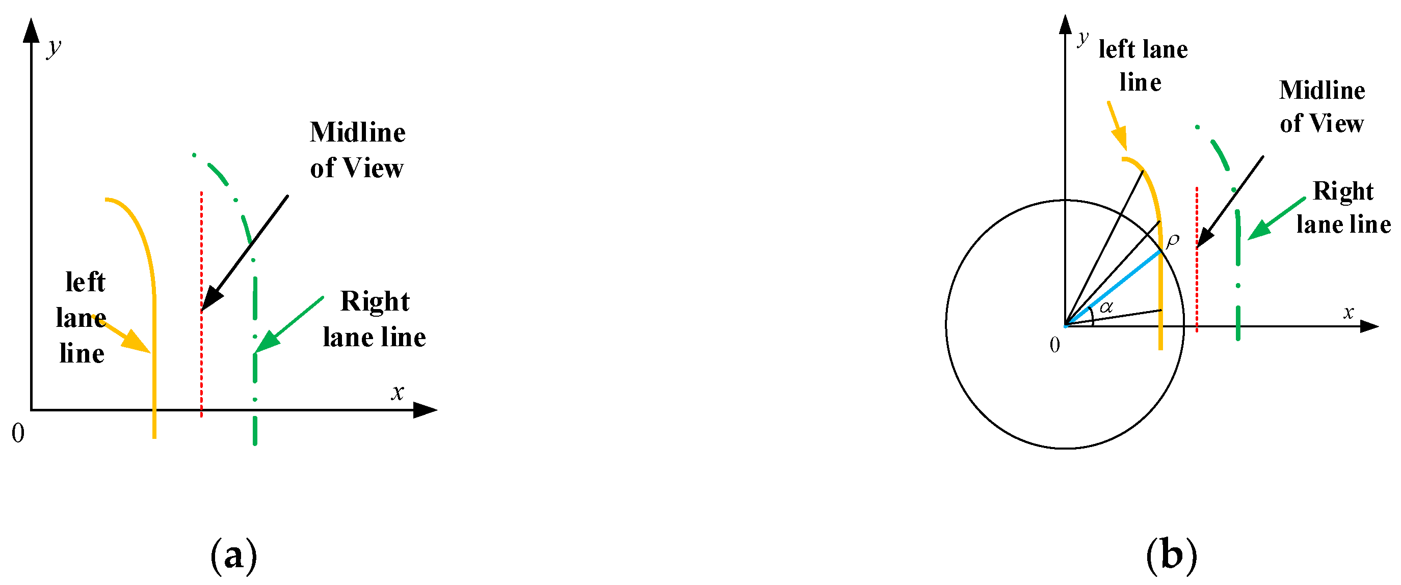
4.5. Lane Line Fitting Based on a Polar Coordinate System

After completing the above steps, the data feature points of the lane lines are available. In this section, the data sets of the left and right lane lines are established, and then the lane line coordinates are estimated by establishing the mathematical model.

A great deal of research has been undertaken on lane line models in the literature. Existing lane line models mainly include the parabolic, linear, hyperbolic, B spline curve and mathematical models of other functions. However, these models are built based on the rectangular coordinate system, and one characteristic of rectangular coordinates is that a given independent variable corresponds to a given dependent variable. In addition, an infinitely sloping lane line cannot be fitted by the equation. In order to solve these problems, the feature points of the lane line are fitted using the polar coordinate system, yielding superior results to those reported using traditional methods.

The shape of the lane line in the image coordinate system is divided into two kinds of straight line and curve. In a Cartesian coordinate system, a given x-coordinate will have multiple values corresponding to the y-coordinate when the lane line is perpendicular to the X-axis. This would violate the definition of linear function, and the lane line could not be represented by the function. To solve this problem, a novel method based on the polar coordinate system is proposed. In this method, the data of the lane line can be fitted by the function $\rho =f\left(\alpha \right)$.

The conditions for the reciprocal transformation of the polar coordinate system and rectangular coordinate system are as follows:

• $\rho \ge 0,\alpha \in \left[0,\pi \right)$.
• The poles of the polar coordinate system coincide with the origin of the rectangular coordinate system.
• The polar axis overlaps with the x axis of the rectangular coordinate system.
• Both coordinate systems have the same unit length.

According to Figure 11, the angle of the lane line in the polar coordinate system varies from 0 to $\mathsf{\pi }$. If the remaining conditions are met, the transformation from the rectangular coordinate system to polar coordinate system can be fulfilled. During lane line fitting, the lane should be divided into straight line fitting and curve line fitting. Additionally, before the ROI is obtained, the differential coefficient should be solved. Based on Equation (26), the feature point (x, y) in the rectangular coordinate system can be transferred to point $\left(\alpha ,\rho \right)$ in the polar coordinate system. Finally, the lane line feature points are fitted by the least square method in the polar coordinate system.

The coordinate transformation relationship is as follows:

$$\{\begin{array}{c}x=\rho \cos \alpha \\ y=\rho \sin \alpha \end{array}$$

(36)

Based on Equation (36), the following fitting equation can be obtained:

$$\{\begin{array}{c}{\rho }_l=f\left({\theta }_l\right)\\ {\rho }_r=f\left({\theta }_r\right)\end{array}$$

(37)

Additionally, according to Equations (14) and (23), the curvature formula can be achieved in the polar coordinate system:

$$\mathrm{K}=\left|\frac{2{{\rho }^{\prime }}^2\left(\theta \right)+{\rho }^2\left(\theta \right)-\rho \left(\theta \right){\rho }^{″}\left(\theta \right)}{{\left({\rho }^2\left(\theta \right)+{{\rho }^{\prime }}^2\left(\theta \right)\right)}^{\frac{3}{2}}}\right|$$

(38)

The curvature radius is represented by:

$$\mathrm{r}=\frac{1}{K}=\left|\frac{{\left({\rho }^2\left(\theta \right)+{{\rho }^{\prime }}^2\left(\theta \right)\right)}^{\frac{3}{2}}}{2{{\rho }^{\prime }}^2\left(\theta \right)+{\rho }^2\left(\theta \right)-\rho \left(\theta \right){\rho }^{″}\left(\theta \right)}\right| ,$$

(39)

where $\beta$ is the inclination of the tangent line at each point below the track, which can be computed by the equation below:

$$\tan \beta =\frac{dy}{dx}=\frac{d\left(\rho \sin \theta \right)}{d\left(\rho \cos \theta \right)}$$

(40)

According the relationship between $\rho$ and $\theta$, $k_t$, the slope of the tangent line at each point of the lane line is solved.

$$k_t=\tan \beta =\frac{{\rho }^{\prime }\left(\theta \right)\sin \theta +\rho \left(\theta \right)\cos \theta }{{\rho }^{\prime }\left(\theta \right)\cos \theta -\rho \left(\theta \right)\sin \theta }$$

(41)

For simplification, $\rho$ and $\theta$ are represented by x and y in the following text. Because the least-squares method has prominent advantages in lane line fitting and high fitting accuracy [26,27], it can realize the fitting of straight lines and curves. In this section, the specific steps of fitting are explained as follows:

Firstly, the approximate curve $y_i=\varnothing \left(x_i\right)$ can be obtained by the given lane line data ${\mathrm{P}}_i\left(x_i,y_i\right)$. At the same time, to ensure the accuracy of the curve, the bias between the obtained equation and the original data point must be minimized. The bias of the curve on the point ${\mathrm{P}}_i\left(x_i,y_i\right)$ is $R^2=\varnothing \left(x_i\right)-y,i=1,2,3,\dots ,n$.

The fitting polynomial is set as follows:

$$\mathrm{y}=a_0+a_{1}x+\dots +a_k{x}^k$$

(42)

The sum of the distance from the feature point of the lane line to the fitting equation is:

$$R^2={\displaystyle \sum }_{i-1}^n{\left[y_i-\left(a_0+a_{1}x+\dots +a_k{x}^k\right)\right]}^2$$

(43)

The partial derivative of $a_i$ is expressed in a simplified form as follows:

$$\{\begin{array}{c}n{a}_0+\left({\displaystyle \sum _i^n}{x}_i\right)a_1+\dots \dots \dots \dots \dots +\left({\displaystyle \sum _i^n}{x}_i{}^k\right)a_k={\displaystyle \sum _i^n}{y}_i\\ \left({\displaystyle \sum _i^n}{x}_i\right)a_1+\left({\displaystyle \sum _i^n}{x}_i{}^2\right)a_2+\dots \dots +\left({\displaystyle \sum _i^n}{x}_i{}^{k+1}\right)a_k={\displaystyle \sum _i^n}{x}_i{y}_i\\ \dots \\ \left({\displaystyle \sum _i^n}{x}_i{}^k\right)a_1+\left({\displaystyle \sum _i^n}{x}_i{}^{k+1}\right)a_2+\dots +\left({\displaystyle \sum _i^n}{x}_i{}^{2k}\right)a_k={\displaystyle \sum _i^n}{x}_i{}^k{y}_i\end{array}$$

(44)

The following equation is achieved after Equation (44) is transformed to the matrix form and simplified:

$$\left[\begin{array}{ccc}1& x_1& \begin{array}{cc}\dots & x_1{}^k\end{array}\\ 1& x_1& \begin{array}{cc}\dots & x_2{}^k\end{array}\\ \begin{array}{c}⋮\\ 1\end{array}& \begin{array}{c}⋮\\ x_1\end{array}& \begin{array}{c}\begin{array}{cc}\ddots & ⋮\end{array}\\ \begin{array}{cc}\dots & x_n{}^k\end{array}\end{array}\end{array}\right]\left[\begin{array}{c}{a}_0\\ a_1\\ \begin{array}{c}⋮\\ a_k\end{array}\end{array}\right]=\left[\begin{array}{c}{y}_1\\ y_2\\ \begin{array}{c}⋮\\ y_n\end{array}\end{array}\right]$$

(45)

Generally, if both sides of the equitation $XA=Y$ are multiplied by the inverse matrix of x, then the value of A can be determined. In addition, the condition of the method is that A should be a square matrix and not a singular matrix. However, in most cases, this condition is not met.

Therefore, the value of A can be solved by multiplying the transpose of X, as shown below:

$$A={(X^{T}X)}^{-1}{X}^{T}Y,$$

(46)

Then, the least square fitting coefficient of A can be obtained based on Equation (46). A is substituted into the polynomial fitting equation to obtain the lane line equation.

5. Experimental Study and Comparative Analysis

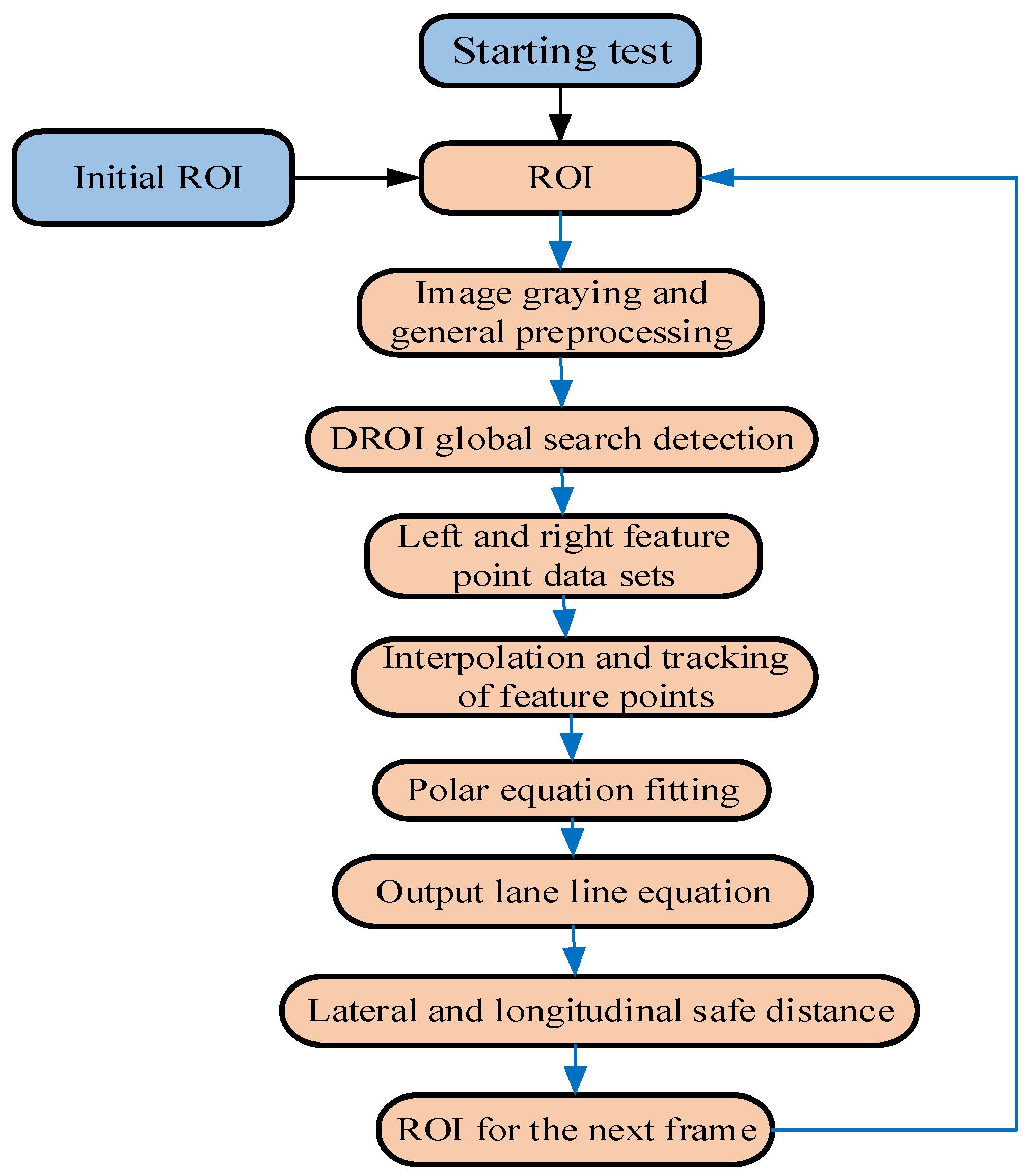
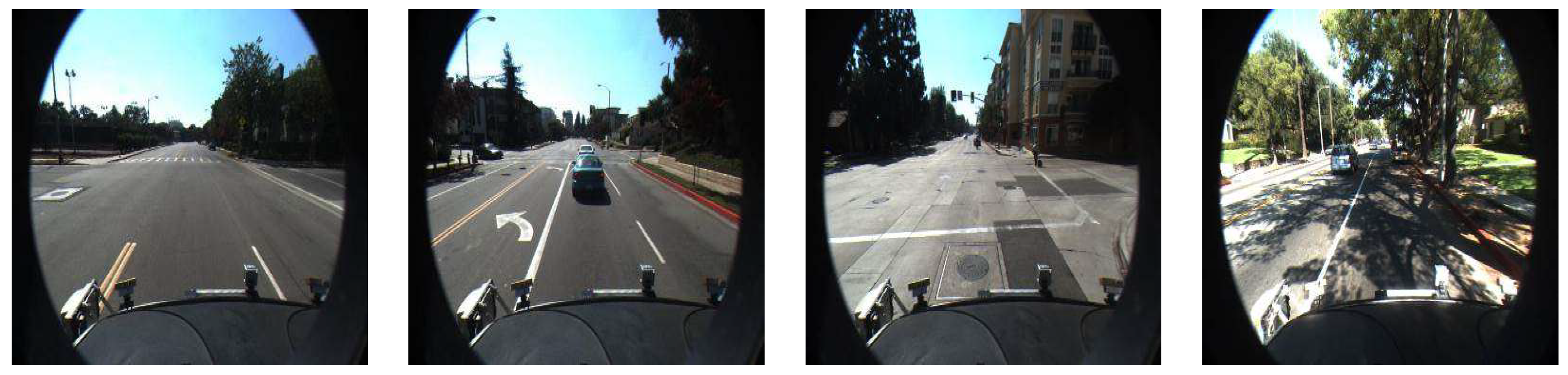
5.1. Experimental Conditions and Algorithm Flow

The novel method of the lane line proposed in the paper is verified using the Matlab 2014a software. The operating hardware environment for lane detection is a computer with Inter(R) Core(TM) i7-6700K CPU. The algorithm flow is shown in Figure 12.

5.2. Evaluation Index of the Lane Line Detection

In order to give an unbiased evaluation for the detection performance of the lane line detection algorithm, this paper utilizes several indicators to evaluate the detection performance [28,29], including the recall rate (the ratio of the number of samples detected correctly in the positive detection to the total number of positive samples), the precision rate (the ratio of the number of samples detected correctly in the positive detection to the number of positive detection), and the missing rate (the ratio of the number of samples detected incorrectly in the negative detection to the total number of positive samples). To obtain the recall rate, precision rate, and missing rate, the true positives (TP), the false positives (FP), the false negatives (FN) and the true negatives (TN) are used. In the lane line detection process, if the detection marks include more than 80% of the lane lines in the DROI, the error is no more than 5 pixels, and there is no other false detection, then the lane line identification is accurate. TP refers to correct detections FP to false detections among the positive detections. FN means the number of samples detected incorrectly in the negative detection. TN refers the number of samples detected correctly in the negative detection. Using TP, FP, TN, and FN, the recall rate, precision rate, and loss rate are given as follows. In addition, Figure 13 shows the corresponding effect diagram:

$$Recall=\frac{TP}{TP+FN}$$

(47)

$$Precision=\frac{TP}{TP+FP}$$

(48)

$$\mathrm{Missing}\mathrm{Rate}=\frac{FN}{TP+FN}$$

(49)

In addition, Figure 13 shows the corresponding effect diagram.

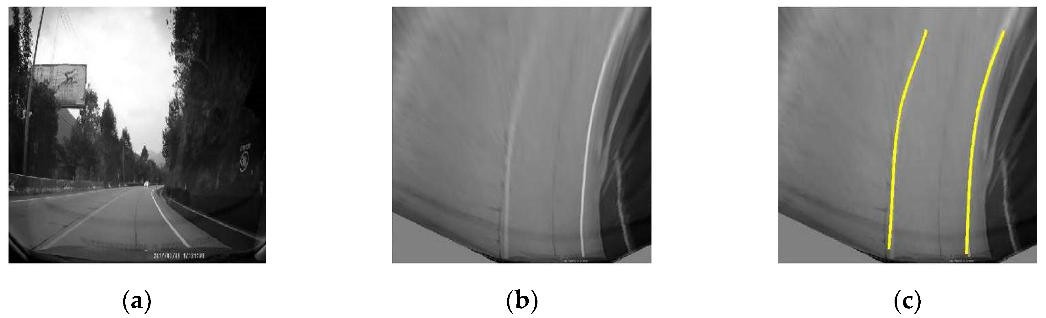
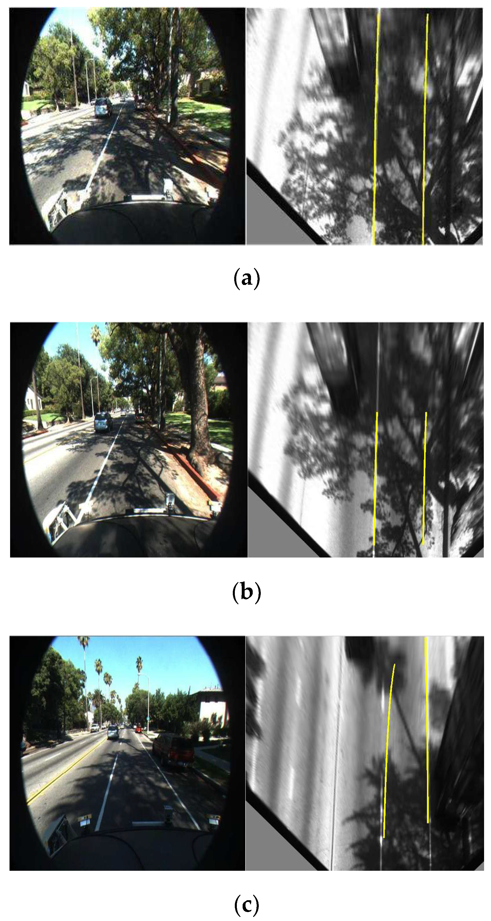
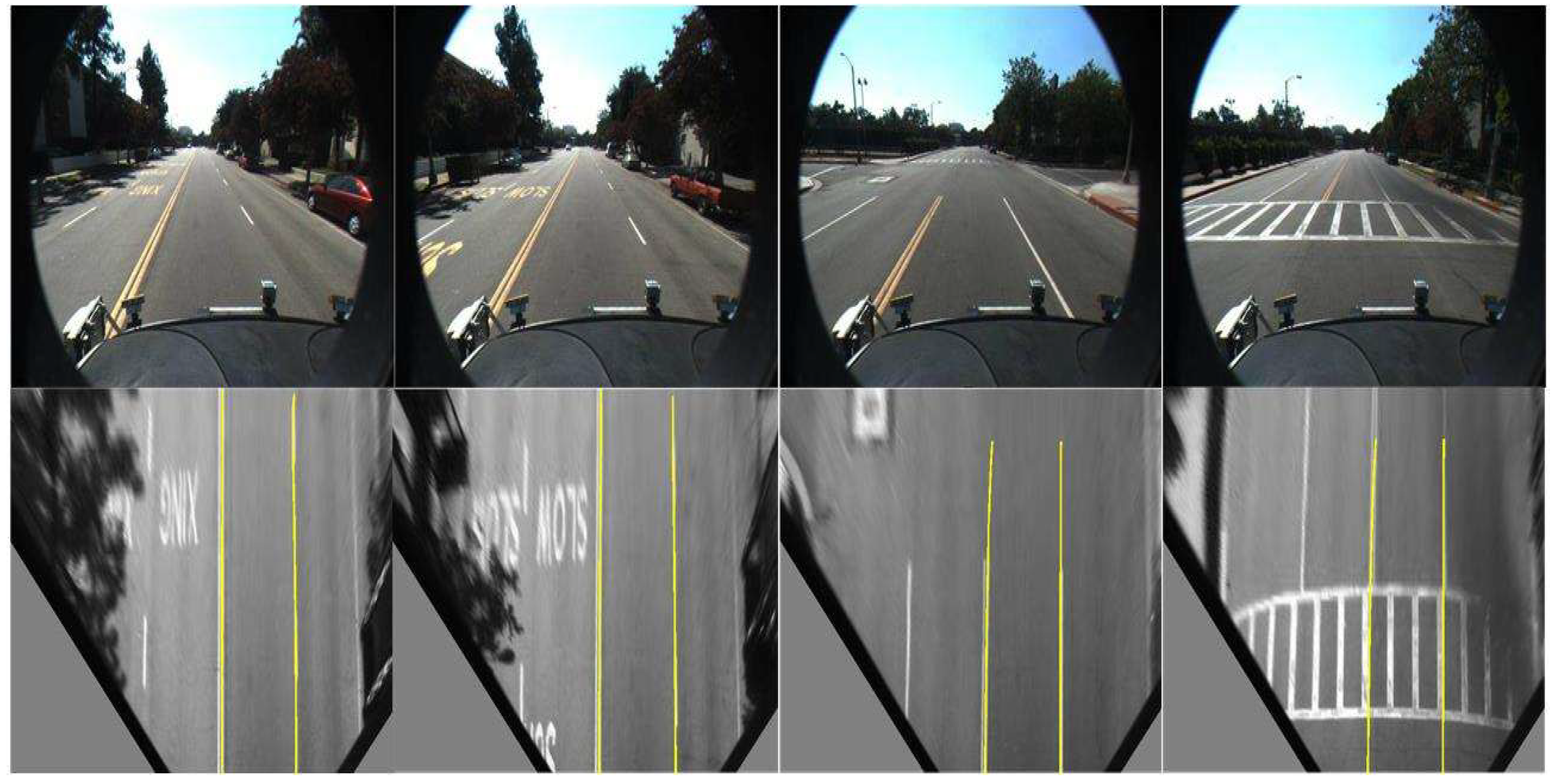
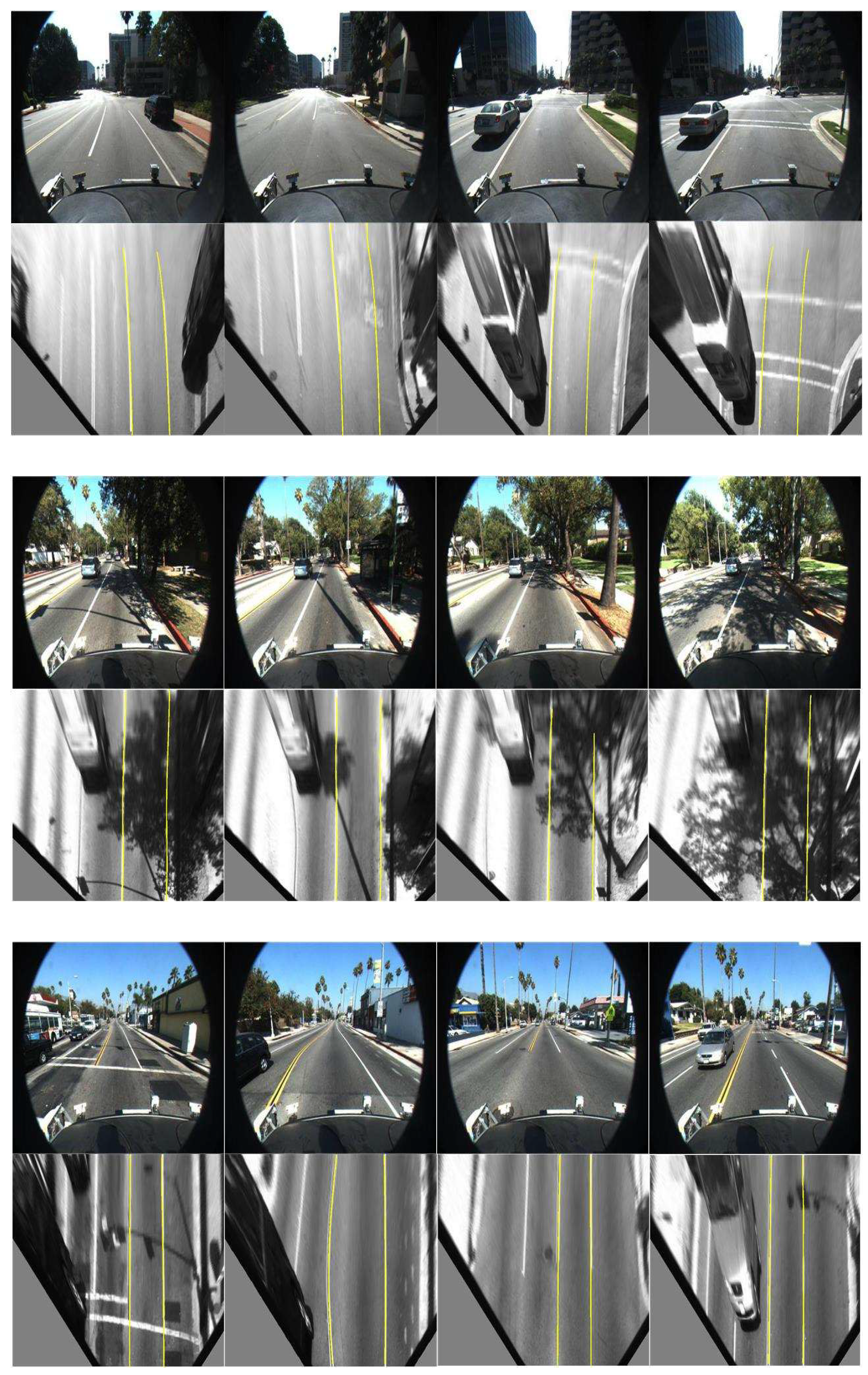
5.3. Comparative Analysis of Test Results

If self-gathered data is used for the verification of lane line detection algorithms, it is hard to evaluate in a common standard. The Caltech datasets are widely utilized because they have not only structured paths, but also unstructured roads including shadows and road marks of varying intensities. Therefore, these data are used to evaluate the algorithm in this paper. Some classic roads are shown in Figure 14.

The Caltech data sets have been used to evaluate various lane line algorithms by numerous researchers around the world. Aly etc. [30] presented a fast lane line detection method based on RANSAC. He etc. [31] put forward an effective lane line detection method based on Hough transform and the Canny algorithm, and a lane marker detection approach based on automobile instantaneous directional enhancement method was proposed by Seo [32]. The proposed method was compared with the above methods using the Caltech data sets, as shown in

Table 2. Detection result comparison.

Methods	Evaluation Index	Cordova1 (250)	Cordova2 (406)	Washington1 (336)	Washington2 (232)
Proposed	Precision (%)	99.6	99.76	98.1	99.57
	Recall rate (%)	99.58	97.5	94.7	98.3
Aly [30]	Precision (%)	97.2	96.2	96.7	95.1
	Recall rate (%)	97	61.8	95.3	97.8
He [31]	Precision (%)	87.6	82.4	74.0	85.1
	Recall rate (%)	74.1	45.2	72.3	74.9
Seo [32]	Precision (%)	87.6	89.1	81.8	88.8
	Recall rate (%)	89.2	90.8	94.7	94.8

.

As shown in Table 2, the detection performance of the proposed method is better than those of the other methods. The main reasons are as follows: in [30], the lane line vanishing point is not easy to choose and there is an absence of lane line, so this method is unsuitable for worn lane lines. The RANSAC algorithm [29] is unsuitable for lane lines with large curvatures. The method proposed by Seo encounters difficulties improving lane line detection according to the driving direction due to the inverse of the lane line. The detection results of the method presented in this paper are shown in Figure 15.

In order to further evaluate the algorithm proposed in this paper, other typical road environments including highways, wet roads, and rural roads are tested. Figure 16 shows some typical road conditions used for evaluation:

Table 3. Detection results of the seed algorithm using other data sets.

Data sets	Weather	Frames	Precision (%)	Missing Rate (%)
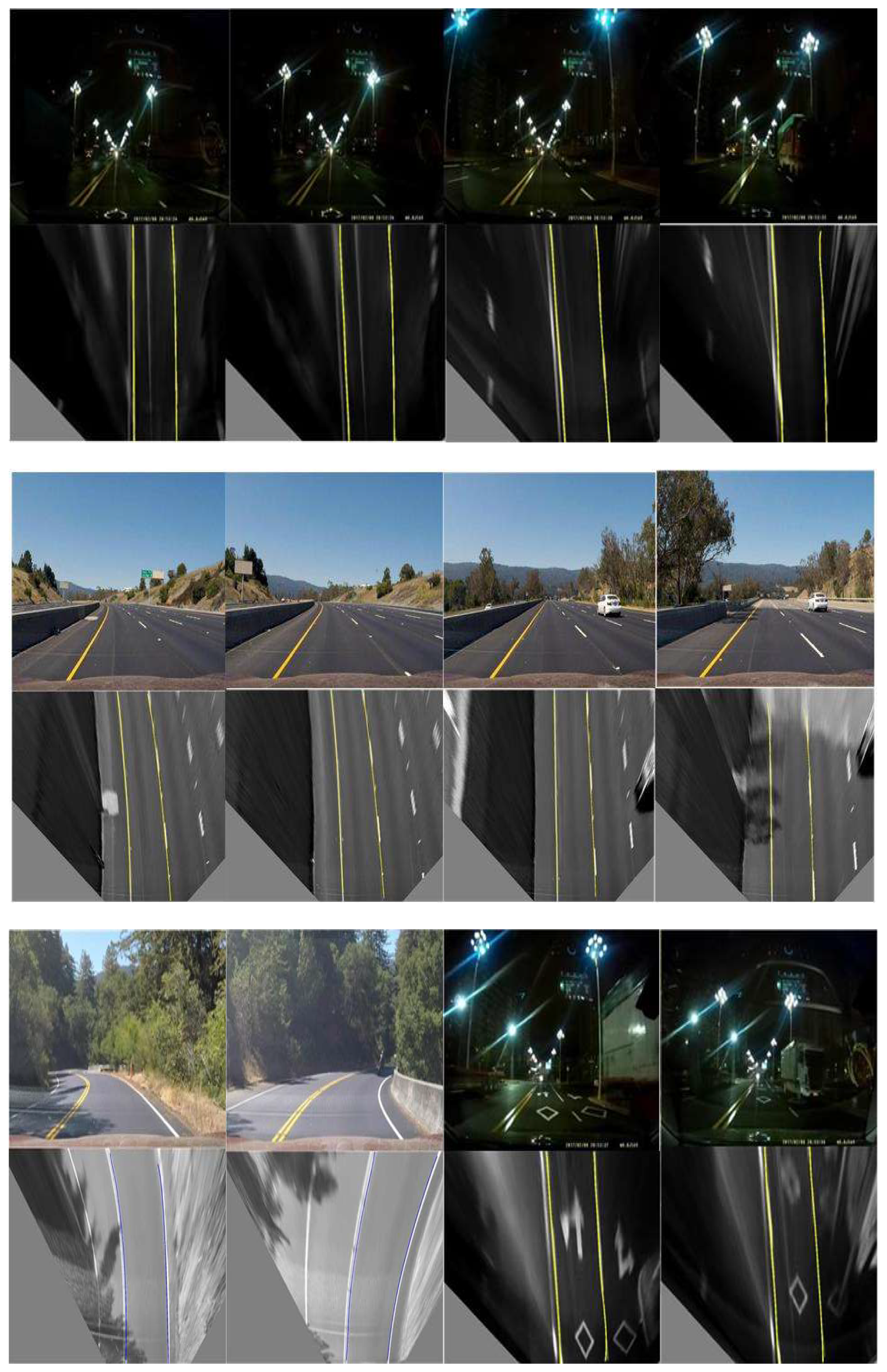
Highways	Day time	1260	99.61	1.2
Rural roads		3214	98.92	1.5
Mountain roads		208	99.1	2.8
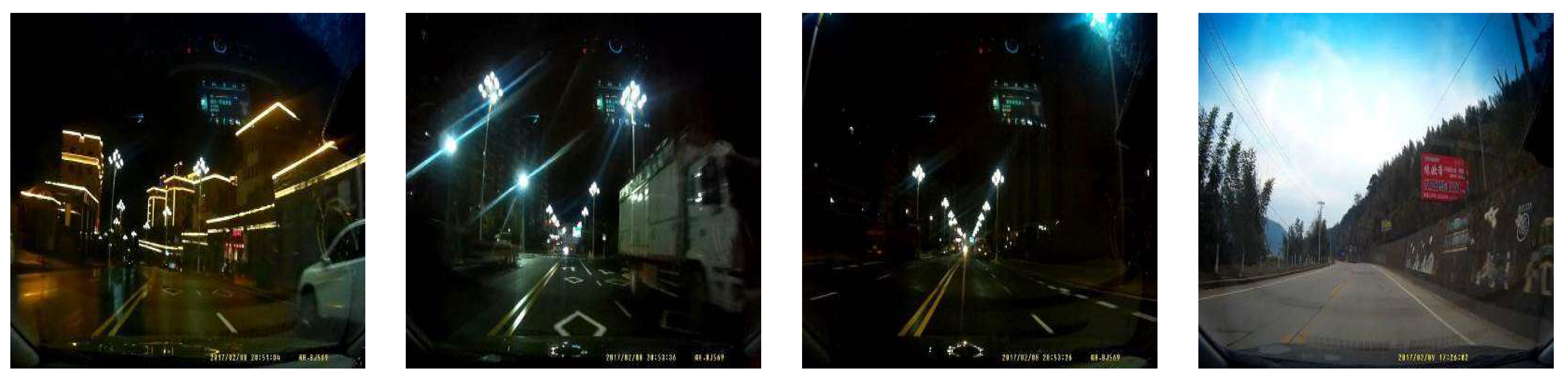
Wet road 1	Night	501	99.0	1.6
Wet road 2		500	99.6	1.2

shows the test results of the proposed detection method under different driving scenarios. It is seen that for all tested driving scenarios, the positive detection rate of the proposed method is close to 99%, and the missing detection rate is less than 3%, which meets the requirements of lane line detection. In addition, Figure 17 shows the test results under different road conditions.

The detection accuracy is improved by adding the constraints described in this paper. In order to avoid affecting the varying curvature of lane lines, the row of the large obstacles including font markings and zebra crossings can be ignored. Furthermore, if there is a lane line on the road, this can be used for other lane line estimation. Lastly, the method proposed in this paper provides good detection results using both classical data sets and complex road conditions data sets, which meets the practical application requirements of road recognition.

6. Discussion of Results

In order to validate the advantages of the proposed algorithm, it was tested using the Caltech data sets. The obtained results demonstrate that the positive detection rate reaches 99.21% and the missing detection rate is about 2.7%, which is superior to other mainstream methods in terms of accuracy.

Furthermore, 5683 frames of road images including highway, rural road, wet roads, and mountain roads during the daytime and at night were further detected using the proposed method. The results show that the positive detection rate reaches 99.07%, while the misdetection rate is lower than 3%, which indicates that the proposed algorithm provides good adaptability in different complex environments.

7. Conclusions

In order to improve the accuracy of lane detection, a novel approach based on DROI selection in the safety vision and lane line fitting in a polar coordinate system is proposed in the paper. The characteristics of lane lines on structured roads are analyzed, and the DROI global search method is used to detect the lane lines. Meanwhile, the interpolation and tracking of lane line feature points are carried out. Given the advantages of the polar coordinate equation fitting curve, the least square method is used to fit the lane line in the polar coordinate system. Lastly, the proposed approach is evaluated using the Caltech database, and the accuracy rate is 99.21%. Additionally, the positive detection rate is shown to be 99.07% in complicated real road environments, which verifies the robustness of the proposed method. The accuracy of this method is clearly superior to those of other mainstream methods.

The approach proposed in this paper has good application prospects in advanced driver assistance systems. In addition, the method of extracting the dynamic region of interest can also be applied in the field of robotics.

References

- Song, W.; Yang, Y.; Fu, M.; Li, Y.; Wang, M. Lane Detection and Classification for Forward Collision Warning System Based on Stereo Vision. IEEE Sens. J. 2018, 18, 5151–5163. [Google Scholar] [CrossRef]
- Rui, S.; Hui, C.; Zhiguang, X.; Yanyan, X.; Reinhard, K. Lane detection algorithm based on geometric moment sampling. Sci. Sin. (Inf.) 2017, 47, 455–467. [Google Scholar]
- Narote, S.P.; Bhujbal, P.N.; Narote, A.S.; Dhane, D.M. A review of recent advances in lane detection and departure warning system. Pattern Recogn. 2018, 73, 216–234. [Google Scholar] [CrossRef]
- Li, C.; Nie, Y.; Dai, B.; Wu, T. Multi-lane detection based on multiple vanishing points detection. In Proceedings of the Sixth International Conference on Graphic and Image Processing (ICGIP 2014), Beijing, China, 24 October 2014. [Google Scholar]
- Ozgunalp, U.; Fan, R.; Ai, X.; Dahnoun, N. Multiple Lane Detection Algorithm Based on Novel Dense Vanishing Point Estimation. IEEE Trans. Intell. Transp. 2017, 18, 621–632. [Google Scholar] [CrossRef]
- Hai, W.; Ying-feng, C.; Guo-yu, L.; Wei-gong, Z. Lane line detection method based on orientation variance Haar feature and hyperbolic model. J. Traffic Transp. Eng. 2014, 5, 119–126. [Google Scholar]
- Chanho, L.; Ji-Hyun, M. Robust Lane Detection and Tracking for Real-Time Applications. IEEE Trans. Intell. Transp. 2018, 19, 4043–4048. [Google Scholar]
- Li, S.; Xu, J.; Wei, W.; Qi, H. Curve lane detection based on the binary particle swarm optimization. In Proceedings of the 29th Chinese Control and Decision Conference (CCDC), Chongqing, China, 28–30 May 2017. [Google Scholar]
- Gaikwad, V.; Lokhande, S. Lane Departure Identification for Advanced Driver Assistance. IEEE Trans. Intell. Transp. 2015, 16, 1–9. [Google Scholar] [CrossRef]
- Yuhao, H.; Shitao, C.; Yu, C.; Zhiqiang, J.; Nanning, Z. Spatial-temproal based lane detection using deep learning. In Proceedings of the IFIP International Conference on Artificial Intelligence Applications and Innovations, Rhodes, Greece, 25–27 May 2018. [Google Scholar]
- Wang, L. Design and Implementation of a Track Detection Algorithm Based on Hyperbolic Model. Master’s Thesis, Jilin University, Changchun, China, 2014. [Google Scholar]
- Kim, J.; Park, C. End-To-End ego lane estimation based on sequential transfer learning for self-driving cars. In Proceedings of the 2017 IEEE Conference on Computer Vision and Pattern Recognition Workshops (CVPRW), Honolulu, HI, USA, 21–26 July 2017. [Google Scholar]
- Longjard, C.; Kumsawat, P.; Attakitmongkol, K.; Srikaew, A. Automatic Lane Detection and Navigation using Pattern Matching Mode. In Proceedings of the International Conference on Signal, Speech and Image Processing, Beijing, China, 15–17 September 2007. [Google Scholar]
- Wang, J.; Gu, F.; Zhang, C.; Zhang, G. Lane boundary detection based on parabola model. In Proceedings of the International Conference on Information and Automation, Harbin, China, 20–23 June 2010. [Google Scholar]
- Zhao, K.; Meuter, M.; Nunn, C.; Muller, D.; Muller-Schneiders, S.; Pauli, J. A novel multi-lane detection and tracking system. In Proceedings of the 2012 Intelligent Vehicles Symposium, Alcala de Henares, Spain, 3–7 June 2012. [Google Scholar]
- Jung, C.R.; Kelber, C.R. An Improved Linear-Parabolic Model for Lane Following and Curve Detection. In Proceedings of the XVIII Brazilian Symposium on Computer Graphics and Image Processing (SIBGRAPI’05), Natal, Rio Grande do Norte, Brazil, 9–12 October 2005. [Google Scholar]
- Jinhe, Z.; Futang, P. A method of selective image graying method. Comput. Eng. 2006, 32, 198–200. [Google Scholar]
- Chen, Q.; Zhao, L.; Lu, J.; Kuang, G.; Wang, N.; Jiang, Y. Modified two-dimensional Otsu image segmentation algorithm and fast realisation. IET Image Process 2012, 6, 426. [Google Scholar] [CrossRef]
- Zijing, W.; Fei, D. Matching method for oblique aerial images based on plane perspective projection. J. Geomat. 2018, 2, 28–31. [Google Scholar]
- Yoo, J.H.; Lee, S.; Park, S.; Kim, D.H. A Robust Lane Detection Method Based on Vanishing Point Estimation Using the Relevance of Line Segments. IEEE Trans. Intell. Transp. 2017, 18, 3254–3266. [Google Scholar] [CrossRef]
- Baozheng, F. Research on Monocular Vision Detection Method of Structured Road Lane. Master’s Thesis, Hunan University, Changsha, China, 2018. [Google Scholar]
- Ming, W. The relation between braking distance and speed. Highw. Automot. Appl. 2010, 3, 46–49. [Google Scholar]
- Dan, Y.; Zhong, Q. Research on Image Segmentation Based on Global Optimization Search Algorithm. Comput. Sci. 2009, 36, 278–280. [Google Scholar]
- Zhi-Fang, L.U.; Bao-Jiang, Z. Image Interpolation with Predicted Gradients. Acta Autom. Sin. 2018, 44, 1072–1085. [Google Scholar]
- Ying, X.; Xiuyan, S. On gray prediction model based on an improved FCM algorithm. Stat. Decis. 2017, 6, 27–30. [Google Scholar]
- Zhudong, L.; Hongyang, C. Lane mark recognition based on improved least squares lane mark model. Automob. Appl. Technol. 2015, 36, 1671–7988. [Google Scholar]
- Sun, P.; Chen, H. Lane detection and tracking based on improved Hough transform and least-squares method. In Proceedings of the International Symposium on Optoelectronic Technology and Application 2014: Image Processing and Pattern Recognition, Beijing, China, 13 May 2014. [Google Scholar]
- Yue, W.; Xianxing, F.; Jincheng, L.; Zhenying, P. Lane line recognition using region division on structured roads. J. Comput. Appl. 2015, 9, 2687–2691. [Google Scholar]
- He, B.; Ai, R.; Yan, Y.; Lang, X. Accurate and robust lane detection based on Dual-View Convolutional Neutral Network. In Proceedings of the 2016 IEEE Intelligent Vehicles Symposium (IV), Gothenburg, Sweden, 19–22 June 2016. [Google Scholar]
- Aly, M. Real time detection of lane markers in urban streets. In Proceedings of the 2008 IEEE Intelligent Vehicles Symposium, Eindhoven, Netherlands, 4–6 June 2008. [Google Scholar]
- He, J.; Rong, H.; Gong, J.; Huang, W. A Lane Detection Method for Lane Departure Warning System. In Proceedings of the 2010 International Conference on Optoelectronics and Image Processing, Haikou, China, 11–12 November 2010. [Google Scholar]
- Seo, Y.; Rajkumar, R.R. Utilizing instantaneous driving direction for enhancing lane-marking detection. In Proceedings of the 2014 IEEE Intelligent Vehicles Symposium Proceedings, Dearborn, MI, USA, 8–11 June 2014. [Google Scholar]