Smoothing and Differentiation of Kinematic Data Using Functional Data Analysis Approach: An Application of Automatic and Subjective Methods

Abstract

Smoothing is one of the fundamental procedures in functional data analysis (FDA). The smoothing parameter $\lambda$ influences data smoothness and fitting, which is governed by selecting automatic methods, namely, cross-validation (CV) and generalized cross-validation (GCV) or subjective assessment. However, previous biomechanics research has only applied subjective assessment in choosing optimal $\lambda$ without using any automatic methods beforehand. None of that research demonstrated how the subjective assessment was made. Thus, the goal of this research was to apply the FDA method to smoothing and differentiating kinematic data, specifically right hip flexion/extension (F/E) angle during the American kettlebell swing (AKS) and determine the optimal $\lambda .$ CV and GCV were applied prior to the subjective assessment with various values of $\lambda$ together with cubic and quintic spline (B-spline) bases using the FDA approach. The selection of optimal $\lambda$ was based on smoothed and well-fitted first and second derivatives. The chosen optimal $\lambda$ was $1\times {10}^{-12}$ with a quintic spline (B-spline) basis and penalized fourth-order derivative. Quintic spline is a better smoothing and differentiation method compared to cubic spline, as it does not produce zero acceleration at endpoints. CV and GCV did not give optimal $\lambda ,$ forcing subjective assessment to be employed instead.

1. Introduction

Signals from motion analysis systems are contaminated with noise or error, resulting from electrical interference in the system, skin motion, and inaccurate data digitization. The noise has features that are different from the actual signal: low amplitude, nondeterministic, and diverse frequency range [1]. Therefore, raw signals or data must be smoothed or filtered to eradicate such noise while preserving the original signal traits. Traditionally, biomechanics data, specifically displacement data, were smoothed to obtain velocity and acceleration using several methods such as polynomial, splines, and Fourier series, as well as digital filtering.

Cubic spline has been proven to be a better smoothing technique than polynomial as a second derivative; that is, the acceleration of displacement data is well-fitted by using cubic spline rather than orthogonal polynomial [2] and Chebyshev polynomial [3]. Polynomial produces an oversmoothed acceleration curve, which provides unrealistic acceleration values in running events [3], and an oversmoothed angular acceleration curve, which attenuates the peaks and falsifies the time histories of single segment motion [4]. However, a higher-order spline, specifically quintic spline, is found to be superior over cubic spline. A comparison between the third derivatives of cubic and quintic spline methods in vertical jump data from Miller and Nelson [5] indicates that quintic spline is a better smoothing technique than cubic spline, and the presence of a discontinuity in the third derivative of cubic spline supports the argument [6]. Quintic spline also produced a well-fitted raw angular displacement film data and its second derivative, as shown in the research of Pezzack et al. [4].

Cubic spline tends to be zero at endpoints of the second derivative of displacement data [3]. This occurrence is known as endpoint error [7], while some identify this term as an endpoint problem [8,9], a boundary effect [10], or an edge effect [11]. Zernicke et al. [2] managed to reduce zero second derivative at endpoints with cubic spline by adding three extra data points at the beginning and end of each dataset. McLaughlin et al. [3] showed that the cubic spline function produced zero acceleration at endpoints for a weight-dropping experiment. Similarly, the vertical acceleration of a dropping golf ball with cubic spline emphasized the presence of zero acceleration at endpoints, which supports quintic spline as a better smoothing method than cubic spline [9].

The superiority of quintic spline is found not only over cubic spline but also over digital filter and Fourier series. Vint and Hinrichs [7] compared four popular smoothing methods, Butterworth digital filter, Fourier series, cubic spline, and quintic spline, in terms of root mean squared (RMS) residual errors of acceleration in endpoint regions using Lanshammar’s [12] modification of Pezzack et al.’s [4] raw angular displacement data. Quintic spline produced the most accurate acceleration values, which was close to the endpoints of the modified Pezzack et al. [4] dataset compared to the other three methods, although none of the methods completely eradicated the endpoint errors [7]. Quintic spline is also the most accurate smoothing method compared to stepwise polynomial regression and simple polynomial regression, although stepwise polynomial regression can be used as an alternative to quintic spline [13].

Nevertheless, all previous methods of smoothing and differentiating raw displacement data mentioned above are in the discrete data form. Analysis using discrete data leads to the discarding of essential features in the data [14,15]. Hence, functional data analysis (FDA) is introduced as a rising alternative statistical method that approaches data analysis from a functional perspective. FDA can transform discrete data into a functional form before proceeding to any form of analysis [16]. Therefore, FDA is applied for thorough time-series analysis, which is in this case a cycle of American kettlebell swing (AKS), for accurate analysis. The process of transforming discrete data into functional form coincides with smoothing. Basically, the discrete data are transformed into a functional form by the linear combination of basis functions. Then, the transformed functions will be smoothed either by using regression analysis (least squares estimation) by minimizing the sum of squared errors or by using a roughness penalty [17]. Several parameter estimations need to be identified: the order of basis functions, number of basis functions, number of knots, knots positions, and smoothing parameter $\lambda .$ These parameters have a significant influence on the degree of data smoothness and fitting, which affects the accuracy of data analysis. The choice of smoothing parameter $\lambda$ can be by either automatic methods, namely, cross-validation (CV) and generalized cross-validation (GCV), or subjective assessment.

Previous studies implemented FDA for smoothing biomechanics data before proceeding with an analysis of vertical jumping [18,19], race walking [15], sit-to-stand movement [20,21], running [14], walking [22,23], lifting tasks [24], and military load carrying [25,26,27,28]. However, none of those biomechanics studies applied CV and GCV prior to subjective assessment in determining the optimal smoothing parameter $\lambda .$ Furthermore, none of those studies demonstrated how the subjective assessment was made. Besides that, research on the application of FDA for smoothing in any weightlifting training data has not been reported.

Thus, the goal of this study is to apply FDA in kinematics data, particularly hip flexion/extension (F/E) angle during AKS, and find the optimal smoothing parameter $\lambda$ by using automatic methods (CV and GCV) prior to subjective assessment and testing with two spline bases, cubic and quintic. The kinematic data particularly hip F/E angle during AKS is chosen as an example of biomechanical data that is used for demonstrating the smoothing and differentiation of kinematic data using an FDA approach.

2. Materials and Methods

2.1. Data Collection

Twenty recreationally active men with a mean age, height, and weight of 21 ± 1 years, 1.72 ± 0.07 m, and 69 ± 7.5 kg, respectively, participated in this research. Subjects signed a written consent before starting the experimental procedure. Subjects were confirmed to be healthy and uninjured. Subjects wore tight outfits and were barefoot to avoid errors or noise during data recording due to the movement of clothing. A total of 16 reflective markers were pinned to the clothing or taped to the skin at locations of anatomical landmarks of the subject’s lower extremity: left heel (LHEE), right heel (RHEE), left toe (LTOE), right toe (RTOE), left ankle (LANK), right ankle (RANK), left tibia (LTIB), right tibia (RTIB), left knee (LKNE), right knee (RKNE), left thigh (LTHI), right thigh (RTHI), left posterior superior iliac (LPSI), right posterior superior iliac (RPSI), left anterior superior iliac (LASI), and right anterior superior iliac (RASI), as shown in Figure 1. Reflective markers with a medium size of 14 mm (in diameter) were used.

This research received approval from the Research Ethics Committee of Universiti Kebangsaan Malaysia (UKM PPI/111/8/JEP-2016-612). Three Vicon Nexus infrared cameras (Vicon Motion Systems Ltd., Oxford, UK) comprising 1 MXF20 and 2 MX3+ models were calibrated at 100 Hz before the movement of reflective markers was captured during AKS. Subjects warmed up and familiarized with AKS before the actual experimental process. Cyclical data have low variability [29,30,31]. In addition, collecting more than three repetitions of data would decrease the standard deviation [30]. For these reasons, the data were recorded cyclically, and the subjects were asked to perform two sets of eight repetitions of AKS with a 16 kg kettlebell (Maxx Arc Kettlebell). Subjects were given two to five minutes of resting time between each set. The recorded data were digitized using a Vicon Nexus motion analysis system software version 1.5.2. The data were filtered using a Woltring filtering routine [32] built in the system software with a predicted mean squared error (MSE) of 10 mm² [33] to attenuate the noise before being exported to Microsoft Excel for further analysis.

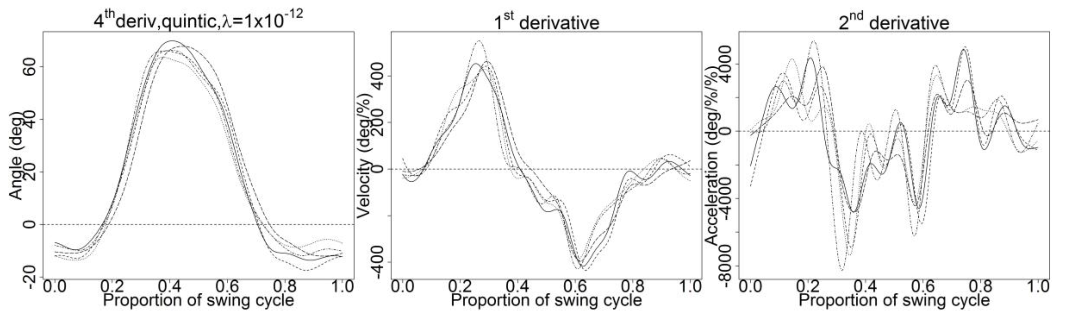
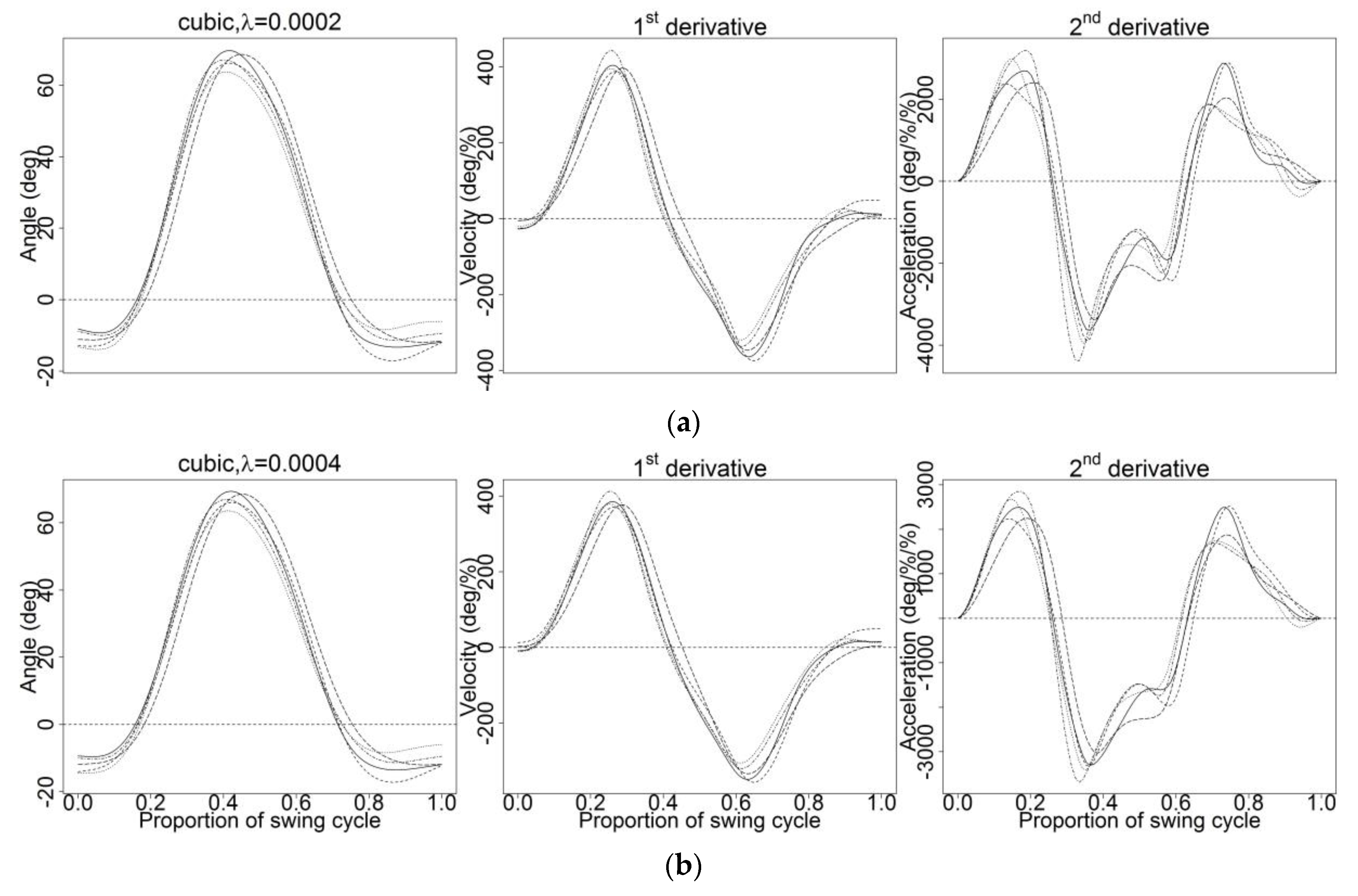
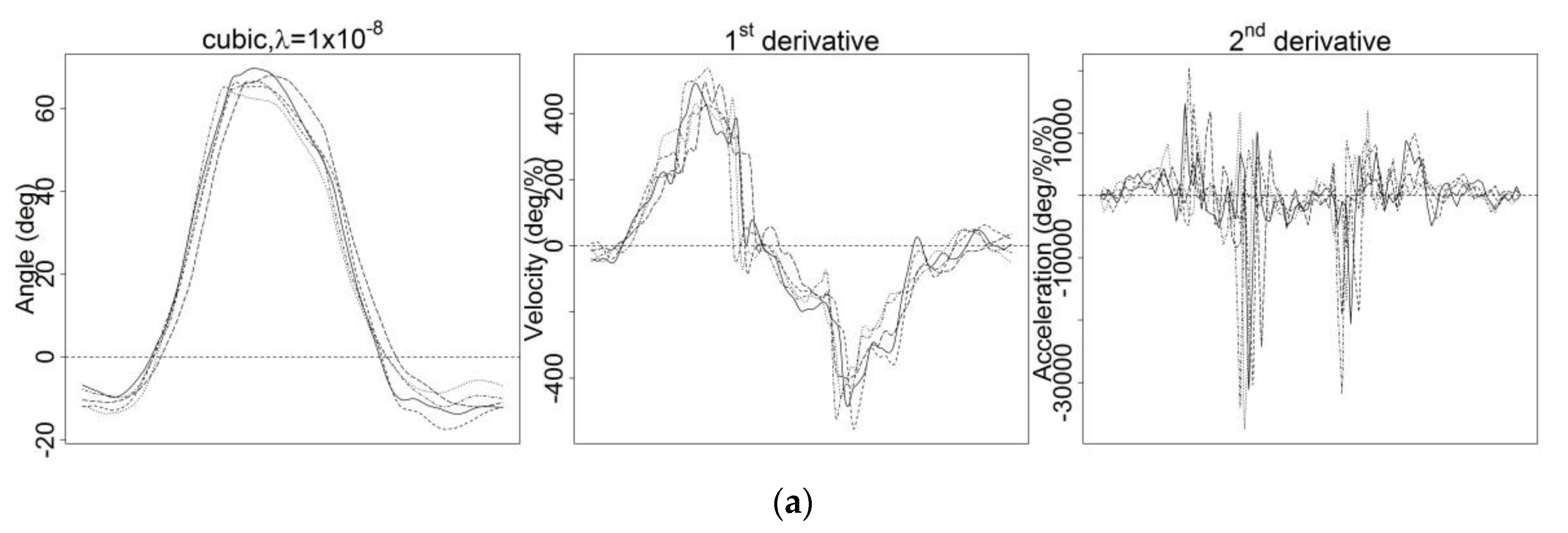
2.2. Derivation of Smooth Functions

Time-normalization was applied prior to any FDA procedures, as in previous research [18,24]. The data were time-normalized to 100 data points. The primary procedure in FDA is to transform discrete data into a functional form. The fda package in R (version 3.4.2) was used for the transformation of discrete data into a functional form and smoothing the functions and the code used is provided in Appendix A.1. R Code A1. The cyclical data were cut into a single cycle of AKS in order to analyze one complete cycle. The cyclical data were cut from the beginning of AKS (stance event) to the end of AKS (propelling kettlebell overhead event) using video recorded in the Vicon Nexus motion analysis system. Each cycle was transformed into a functional form. The data were assumed to have some noise or measurement error, which was assumed to be normally distributed. The data were expressed by the equation:

$$y_j=x(t_j)+{\epsilon }_j,$$

(1)

where $y_j$ is the raw data, $x(t_j)$ is the signal, and ${\epsilon }_j$ is the noise or measurement error.

A set of functional building blocks ${\varphi }_k$ with k = 1, …, K termed as basis functions were combined linearly [16]. The larger the number of K, the closer these functions were to the exact interpolation of the data, whereas the smaller the number of K, the smoother the data. A smaller number of K increases the residual difference between the smooth function and noisy data [1]. The smooth function $x(t)$ was represented as a linear combination of basis functions:

$$x(t)={\displaystyle \sum _{k=1}^K{c}_k{\varphi }_k(t),}$$

(2)

where ${\varphi }_k(t)$ is the k^th basis function at time t, $c_k$ is the coefficient of the expansion, and K is the number of basis expansion [16]. There are several basis functions available—Fourier, B-spline, wavelet, exponential and power, polynomial, polygonal, step-function, constant (single), empirical, and designer bases functions—but the first two are the most commonly used [34]. The use of a basis function depends on the nature of the data. Basically, the Fourier basis function is used for periodic or cyclical functions, while the B-spline basis function is used for nonperiodic functions. The B-spline basis function was chosen since the cyclical data had been cut into individual cycles to portray the behavior of a complete cycle of AKS. The B-spline basis function is one of the most prominent spline functions besides M-spline, I-spline, and truncated power function [35]. It is numerically stable and flexible, which makes it the most frequently used basis function [36]. B-spline was a popular choice among previous researchers as the basis function [15,18,19,22,23,24,37]. There is no universal basis function that is suitable for all types of data.

The spline basis function is a piecewise polynomial made up of divided internal observations to form subintervals with boundaries at points known as break points or breaks [16]. Knots are placed at breaks and are usually equally spaced. However, excessive knots form overfitted data, while fewer knots form underfitted data [38]. The order of a polynomial must be one point higher than its degree. By default, the order of spline is four; thus, the degree is three, which implies a cubic polynomial. Finding the first and second derivatives, velocity and acceleration, is the usual practice in biomechanics. The spline basis must be at least two orders higher than the highest-order derivative that is used [16]. Since order two is the highest order of the derivative of interest (acceleration), a minimum of order four of the spline basis needs to be used. The number of basis functions K is the summation of orders and the number of interior knots in the curve [16]. The interior knots refer to the knots at breaks, excluding the ones at the beginning and end of a function’s domain. Since a large K (K = 100) was used, thus, the number of equally spaced interior knots was 98. A total of 98 equally spaced interior knots were used as a large K (K = 100) was used. The justification for choosing a large K will be explained in the next subsection.

2.3. Regression Analysis and Roughness Penalty

After defining the basis functions and the coefficients required to express the function as a linear combination of the basis functions, the coefficients can be computed using two methods of smoothing functional data: least squares estimation and roughness penalty. Least squares estimation using B-spline basis expansion, which is also known as regression spline smoothing, might work for a simpler linear problem but not for a complex problem. Normally, data fitting is done by minimizing the least squares estimation or sum of squared error, which is denoted as

$$\mathrm{SSE}(x)={\displaystyle \sum _{j=1}^n{\left[y_j-x(t_j)\right]}^2.}$$

(3)

A function x that is described as a basis function expansion (Equation (2)) is known as

$$\mathrm{SSE}(x)={\displaystyle \sum _{j=1}^n{\left[y_j-{\displaystyle \sum _{k=1}^K{c}_k{\varphi }_k(t)}\right]}^2},$$

(4)

where ${\varphi }_k(t),c_k$ and K are defined as in Equation (2). The standard deviation of the residuals, which is the root mean squared error (RMSE), is denoted as

$$\mathrm{RMSE}(x)=\sqrt{\frac{{\displaystyle \sum _{j=1}^n{\left[y_j-x(t_j)\right]}^2}}{n}},$$

(5)

which is a measure of the differences between the values predicted by an estimator, $y_j$ and the values observed, $x(t_j).$

The regularization approach, also known as the roughness penalty, is viewed as a more comprehensive smoothing method [34]. Therefore, it was chosen over regression analysis or least squares estimation for this research. The roughness penalty method uses a large number of basis functions K, while the regression spline uses a smaller K. Thus, a large number of basis functions, K = 100, was chosen, which is equal to the number of data points, n. The raw functional data can be smoothed by adjusting the number of basis functions K. Setting a smaller K induces smoother data but causes the elimination of important functional features. In contrast, setting K = n (n is the number of data points) induces the data to be an exact interpolation, which leads to undersmoothed and overfitted data. However, data overfitting caused by setting K = n is fixed by the roughness penalty term, which penalizes the curvature of the estimated function. This term is controlled by a smoothing parameter $\lambda .$ In the roughness penalty method, the roughness of a fitted curve is measured by finding x that minimizes the penalized residual sum of squares error, as follows:

$$\begin{array}{ll}\mathrm{PENSSE}& ={\displaystyle \sum _{j=1}^n{\left[y_j-x(t_j)\right]}^2+\lambda \times {\mathrm{PEN}}_m}\\ & ={\displaystyle \sum _{j=1}^n{\left[y_j-x(t_j)\right]}^2+\lambda \times {{\displaystyle \int \left[D^{m}x(t)\right]}}^{2}dt},\end{array}$$

(6)

where PENSSE refers to the penalized residual sum of squares error, ${\displaystyle \sum _{j=1}^n{\left[y_j-x(t_j)\right]}^2}$ is the least squares estimation, ${\mathrm{PEN}}_m(x)={{\displaystyle \int \left[D^{m}x(t)\right]}}^{2}dt$ denotes the integrated squared m-order derivative of $x(t),$ and $\lambda$ is the smoothing parameter. In order to measure acceleration, the penalized fourth-order derivative was used, since two order derivatives higher than the desired parameter are needed to be penalized [39].

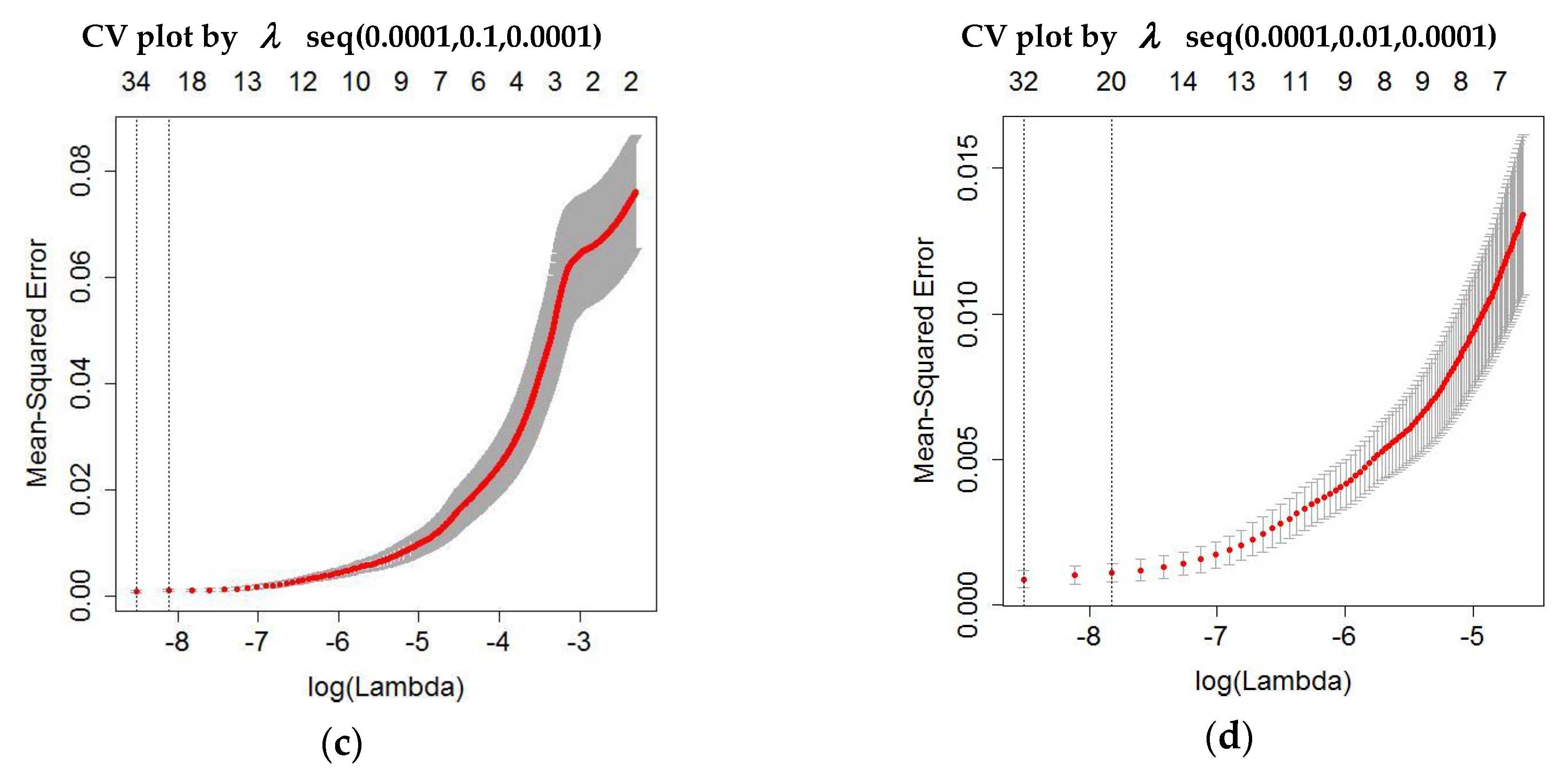
2.4. Cross-Validation and Generalized Cross-Validation

The preference for smoothing parameter $\lambda$ is crucial for selecting the best fit and smoothest curve. When $\lambda$ increases, stress is imposed on the smoothness of the curve but less on the fitting of the curve, whereas when $\lambda$ decreases, stress is imposed on the fitting of the curve but less on the smoothness. When $\lambda =0,$ it indicates that a least squares fit is applied. The smoothing parameter $\lambda$ can be chosen either by automatic or subjective techniques. There are two methods of selecting $\lambda$ automatically, cross-validation (CV) and generalized cross-validation (GCV), as initiated by Craven and Wahba [40]. These methods allow the data to choose the value of $\lambda .$ The principle of CV is denoted by

$$\mathrm{CV}(\lambda )={{\displaystyle \sum _{i=1}^N\left[y_i-{\alpha }_{\lambda }^{(-i)}-{\displaystyle \int x_i(t){\beta }_{\lambda }^{(-i)}dt}\right]}}^2,$$

(7)

where ${\alpha }_{\lambda }^{(-i)}$ and ${\beta }_{\lambda }^{(-i)}$ are estimated regression parameters approximated without the i^th observation [16]. GCV, a simpler method, was developed after CV, as it is more reliable and data undersmoothing is unlikely to take place [34]. The principle of GCV is expressed as

$$\mathrm{GCV}(\lambda )=\left(\frac{n}{n-df(\lambda )}\right)\left(\frac{\mathrm{SSE}}{n-df(\lambda )}\right),$$

(8)

where df is the degrees of freedom for spline smoothing n times [16].

However, it is suggested that an automatic method such as CV be used as a guide rather than a fixed rule prior to using a subjective method to select $\lambda$ [36]. Nevertheless, the credibility of these two methods was tested. Both CV and GCV methods were analyzed using the glmnet package in R, and the codes are provided in Appendix A.2. R Code A2 and Appendix A.3. R Code A3, respectively. The subjective technique used referred to the first and second derivatives, velocity and acceleration. The rule was to find an optimal $\lambda$ and spline basis that smoothed the derivatives while maintaining similar trends or original traits of the derivatives obtained from the graph of the functional data object created (Figure 2b) and the smallest value of $\lambda$ that preserved the original pattern of the curve (Figure 2c).

3. Results and Discussions

Several tests were conducted to identify the optimal smoothing parameter $\lambda$ on a total of 100 trials from 20 subjects (five trials per subject). The noise or measurement error might not be obviously visible in the raw data, but they will be amplified in the derivatives. For this reason, the first and second derivatives were used as indicators for determining the optimal smoothing parameter $\lambda .$ The right hip F/E angle and its respective first and second derivatives were plotted side by side, and only five trials of right hip F/E angle from a subject during AKS were displayed for a clear view of the effect of smoothing parameter $\lambda .$ Figure 2a shows the raw right hip F/E angle in a discrete form during AKS. Noise did exist, but it was not very noticeable (Figure 2a). The transformation of discrete data into a functional form and smoothing occurred simultaneously. Therefore, by default, a functional data object with class name fd was created. The graph of the functional data object is plotted in Figure 2b. Since the second-derivative curves plotted in Figure 2b are unclear, several trials were performed to find the smallest value of $\lambda$ that preserved the original pattern of the curves referred to in Figure 2b. As a result, the smallest value of $\lambda$ that preserved the original pattern of the curves were found to be $\lambda =1\times {10}^{-21},$ as shown in Figure 2c. The first and second-derivative curves in Figure 2c were used as references in choosing the optimal smoothing parameter $\lambda .$

The automatic methods, CV and GCV, were applied to the raw right hip F/E angle data to obtain $\lambda .$ First, the data were tested with the CV method. The CV plot of mean squared error (MSE) corresponding to the smoothing parameter $\lambda$ that was generated by default using the glmnet package in R was plotted, as shown in Figure 3a. By default, the number of folds is 10 and the alpha is 1. The other CV plot of MSE of the range of $\lambda$ sequences—seq(0, 1, 0.0001), seq(0.0001, 0.1, 0.0001), and seq(0.0001, 0.01, 0.0001)—were plotted, as shown in Figure 3b–d, respectively.

The red dotted line is the CV curve and the error bars along the $\lambda$ sequences are upper and lower standard deviation curves (95% confidence interval). The y-axis represents the MSE for respective values of $\lambda ,$ while the upper x-axis represents the number of predictors. The two vertical dotted lines are two choices of smoothing parameter $\lambda ,$ which are the value of $\lambda$ that gives the minimum cross-validated error and the largest value of $\lambda$ that gives the most regularized model where the error is within one standard error of the minimum. The first choice of $\lambda$ would give the most accurate model, while the second choice would also give a good accurate model with the smallest number of predictors. Thus, both $\lambda$ values were considered for optimal $\lambda .$ As the number of predictors decreased, the MSE increased gradually. The number of predictors stabilized after a certain number of predictors was added. However, the MSE of Figure 3a started to make the increasing pattern less steep at around ${\log }_{10}(\lambda )=-3$, as there were fewer predictors. The MSE in Figure 3a started to stabilize upon reaching ${\log }_{10}(\lambda )<-6.$ Since the MSE stopped at ${\log }_{10}(\lambda )$ not more than approximately $-6.7$ (Figure 3a), thus, a wider range of $\lambda$ sequences was tested to determine the optimal $\lambda$ with a wider $\lambda$ interval. Several range of lambda with various sequences were tested in order to determine the optimal $\lambda$ with a wider $\lambda$ interval, as shown in Figure 3b–d. Both choices of $\lambda$ (vertical dotted lines) were invisible, as both were 0 using seq(0, 1, 0.0001) (Figure 3b). Therefore, a smaller sequence, seq(0.001, 0.1, 0.0001) (Figure 3c) was tested and resulted in a wider range of $\lambda$ with the two choices of $\lambda$ as 0.0002 and 0.0003. The range of $\lambda$ sequence in Figure 3d shows a well-adjusted ${\log }_{10}(\lambda )$ range approximately less than $-4$ and greater than $-8.5$, although the MSE leveled off at around ${\log }_{10}(\lambda )$ not more than $-9.$ The MSE increased steadily as the number of predictors decreased. For the two choices of $\lambda$ from Figure 3d, the value of $\lambda$ that gives the minimum cross-validated error and the largest value of $\lambda$ that gives the most regularized model where the error is within one standard error of the minimum are 0.0002 and 0.0004, respectively. These values were tested, and their first and second-derivative curves were plotted side by side, as shown in Figure A1.

By default, the order of a spline is four, which implies a cubic spline basis [16]. It clearly shows that the CV method could not be utilized to determine a suitable $\lambda ,$ as both values of $\lambda$ oversmoothed the first and second-derivative curves (Figure A1). Further testing with the quintic spline basis for $\lambda$ driven from the CV method would be unnecessary, because testing with quintic, a higher polynomial than the cubic with the same $\lambda$ driven from the CV method, would yield data oversmoothing. Subsequently, the other automatic method, GCV, was tested for its relevancy. Several values of $\lambda$ were tested, and the graphs of degrees of freedom (df), root mean squared error (RMSE), and GCV were illustrated in Figure 4 and the data collected were tabulated in

Table 1. Various values of $\lambda$ with their respective df, RMSE, and GCV.

${\mathbf{log}}_{10}(\mathit{\lambda })$	Degrees of Freedom (df)	RMSE	GCV
−12	100	35.859	0.038
−11	100	35.859	0.038
−10	100	35.859	0.037
−9	98	35.859	0.036
−8	86	35.858	0.032
−7	60	35.858	0.046
−6	36	35.852	0.146
−5	21	35.824	0.578
−4	12	35.667	2.637
−3	7	34.839	14.704

.

According to Figure 4 and Table 1, the value of $\lambda =1\times {10}^{-8}$ recorded the smallest GCV, 0.032, among the other $\lambda$ values tested. At this smoothing level, the degrees of freedom measure has a value of 86, which is not far from the number of basis functions that were used, 100. The standard deviation of RMSE over the range of $\lambda$ values studied was small. The value of $\lambda =1\times {10}^{-8}$ that gave the minimum GCV value was tested by plotting its derivative curves (Figure A2).

Some spikes and noise in the first and second-derivative curves could be observed by smoothing with $\lambda =1\times {10}^{-8}$, which was provided by the GCV method using the cubic spline basis (Figure A2a). Additional testing with the quintic spline basis resulted in oversmoothed first and second-derivative curves (Figure A2b). Apparently, smoothing with $\lambda$ driven by the automatic methods, (CV and GCV), failed to generate a suitable smoothing parameter $\lambda .$ These results were proven to comply with the recommendation from Ramsay and Silverman [36] that an automatic method such as CV should be used as a guide rather than a fixed rule prior to making a subjective assessment in choosing $\lambda .$

For these reasons, subjective assessment was applied to the raw data. The raw data were tested with smoothing parameter $\lambda$ with the values $1\times {10}^{-6},1\times {10}^{-5},1\times {10}^{-4},$ and $1\times {10}^{-3}$ with order four (cubic spline basis) (Figure A3). These values were chosen because testing with $\lambda =1\times {10}^{-8}$ by GCV and the cubic spline basis produced undersmoothed first and second-derivative curves (Figure A2a). Therefore, sets of $\lambda$ with higher values than $1\times {10}^{-8}$ were applied to the raw data (Figure A3). Smoothing using $\lambda =1\times {10}^{-6},$ resulted in undersmoothed first and second-derivative curves (Figure A3a). Noise and fluctuations in the derivative curves remained when smoothing using $\lambda =1\times {10}^{-5},$ although some noise was reduced tremendously as the value of $\lambda$ increased (Figure A3b). The right hip F/E angle and its first and second-derivative curves were indeed smoother as higher $\lambda$ values were used. However, as $\lambda$ reached $1\times {10}^{-4},$ they started to lose the pattern and original traits of the raw data, which might have had a significant effect on interpretation of the data (Figure A3c). Using a higher $\lambda ,$ $1\times {10}^{-3},$ resulted in oversmoothed first and second-derivative curves (Figure A3d). It appeared that for all $\lambda$ tested with the cubic spline basis, the corresponding second-derivative curves, specifically angular acceleration curves, were all zero at endpoints. This occurrence is predictable, as cubic spline tends to have zero acceleration at endpoints [3].

Hence, none of the smoothing parameters demonstrated satisfactory results, forcing the use of a higher-order spline basis. Accordingly, the quintic spline basis (order six) was used for a better result, and several $\lambda$ values were tested: $1\times {10}^{-13},1\times {10}^{-12},1\times {10}^{-11},$ and $1\times {10}^{-10}$ (Figure A4). These values were chosen because a higher polynomial (quintic spline basis) requires a smaller $\lambda$ value than the cubic spline basis. Thus, sets of smaller values of $\lambda$ than $1\times {10}^{-6}$ were applied to the raw data (Figure A4). The second-derivative curves still had a few fluctuations when the quintic spline basis and $\lambda =1\times {10}^{-13}$ were applied (Figure A4a), while the second-derivative curves showed well-fitted and smoothed curves and maintained the original traits of the curves when the quintic spline basis and $\lambda =1\times {10}^{-12}$ were applied (Figure A4b). As $\lambda$ increased, the second-derivative curves became smoother but lost a bit of their pattern when $\lambda =1\times {10}^{-11}$ was used (Figure A4c). Testing with higher $\lambda ,1\times {10}^{-10}$ resulted in oversmoothed first and second-derivative curves (Figure A4d). Compared with the cubic spline basis in Figure A3, smoothing using the quintic spline basis for all $\lambda$ tested in Figure A4 resulted in non-zero angular accelerations at endpoints, which was different from the cubic spline basis. In order to avoid endpoint error, quintic spline was chosen rather than cubic spline.

Although the test showed that the quintic spline basis and $\lambda$ value of $1\times {10}^{-12}$ were the optimal smoothing parameters by far, the effect of penalizing the curve using the roughness penalty was examined. In order to penalize the curvature of the second derivative, the curves should be penalized with the fourth-order derivative [16]. Using the roughness penalty approach, the curves were smoothed using the quintic spline basis, $\lambda$ value of $1\times {10}^{-12}$ and penalized with second and fourth-order derivatives. Penalizing the curves with second-order derivative failed to yield smoothed first and second-derivative curves (Figure A5), whereas penalizing the curves with fourth-order derivative with the same parameters yielded smoothed first and second-derivative curves (Figure 5). Thus, the optimal smoothing parameters were those of a quintic spline (B-spline) basis, which were penalized with fourth-order derivative, and $\lambda$ value of $1\times {10}^{-12}.$ These smoothing parameters were tested and applied for all trials from the other 19 subjects for further analysis (Figure 6).

4. Conclusions

The use of FDA in smoothing kinematics data of AKS involves the transformation of discrete data into a functional form. The smoothing parameter $\lambda$ affected the degree of data smoothness and fitting, which was governed by the automatic methods, CV and GCV, or subjective assessment. The optimal smoothing parameter $\lambda$ for smoothing and differentiating right hip F/E angle during AKS was found to be $1\times {10}^{-12},$ along with other parameters, quintic spline (B-spline) basis and penalized fourth-order derivative. Quintic spline is a better smoothing and differentiation method than cubic spline, as it does not produce zero acceleration at endpoints. Neither of the automatic methods, (CV and GCV) that were applied provided the optimal smoothing parameter, leading to the use of an alternative assessment. These findings might be used as a reference to future biomechanics research to apply automatic methods, CV and GCV, before making a subjective assessment in smoothing and differentiating other biomechanical data using the FDA approach. Although the study found the optimal smoothing parameter for smoothing and differentiating kinematics data of AKS while maintaining the original traits of the data, it was not determined how smoothed data by various values of $\lambda$ would affect the results of further analysis. Therefore, further studies are necessary to determine the effects of smoothed kinematics data of AKS by various values of $\lambda$ on the variability of functional principle component analysis (FPCA).

References

1. Robertson, G.; Caldwell, G.; Hamill, J.; Kamen, G.; Whittlesey, S. Research Methods in Biomechanics, 2nd ed.; Human Kinetics: Champaign, IL, USA, 2014. [Google Scholar]
2. Zernicke, R.F.; Caldwell, G.; Roberts, E.M. Fitting biomechanical data with cubic spline functions. Res. Q. Am. All. Health Phys. Educ. Rec. 1976, 47, 9–19. [Google Scholar] [CrossRef]
3. McLaughlin, T.M.; Dillman, C.J.; Lardner, T.J. Biomechanical analysis with cubic spline functions. Res. Q. Am. All. Health Phys. Educ. Rec. 1977, 48, 569–582. [Google Scholar] [CrossRef]
4. Pezzack, J.C.; Norman, R.W.; Winter, D.A. An assessment of derivative determining techniques used for motion analysis. J. Biomech. 1977, 10, 377–382. [Google Scholar] [CrossRef]
5. Miller, D.I.; Nelson, R.C. Biomechanics of Sport; Lea and Febiger: Philadelphia, PA, USA, 1973. [Google Scholar]
6. Wood, G.A.; Jennings, L.S. On the use of spline functions for data smoothing. J. Biomech. 1979, 12, 477–479. [Google Scholar] [CrossRef]
7. Vint, P.F.; Hinrichs, R.N. Endpoint error in smoothing and differentiating raw kinematic data: An evaluation of four popular methods. J. Biomech. 1996, 29, 1637–1642. [Google Scholar] [CrossRef]
8. Phillips, S.J.; Roberts, E.M. Spline solution to terminal zero acceleration problems in biomechanical data. Med. Sci. Sports Exerc. 1983, 15, 382–387. [Google Scholar] [CrossRef]
9. Vaughan, C.L. Smoothing and differentiation of displacement-time data: An application of splines and digital filtering. Int. J. Bio-Med. Comput. 1982, 13, 375–386. [Google Scholar] [CrossRef]
10. Woltring, H.J. On optimal smoothing and derivative estimation from noisy displacement data in biomechanics. Hum. Mov. Sci. 1985, 4, 229–245. [Google Scholar] [CrossRef]
11. D’amico, M.; Ferrigno, G. Technique for the evaluation of derivatives from noisy biomechanical displacement data using a model-based bandwidth-selection procedure. Med. Biol. Eng. Comput. 1990, 28, 407–415. [Google Scholar] [CrossRef]
12. Lanshammar, H. On practical evaluation of differentiation techniques for human gait analysis. J. Biomech. 1982, 15, 99–105. [Google Scholar] [CrossRef]
13. Burkholder, T.J.; Lieber, R.L. Stepwise regression is an alternative to splines for fitting noisy data. J. Biomech. 1996, 29, 235–238. [Google Scholar] [CrossRef]
14. Donoghue, O.A.; Harrison, A.J.; Coffey, N.; Hayes, K. Functional data analysis of running kinematics in chronic Achilles tendon injury. Med. Sci. Sports Exerc. 2008, 40, 1323–1335. [Google Scholar] [CrossRef]
15. Dona, G.; Preatoni, E.; Cobelli, C.; Rodano, R.; Harrison, A.J. Application of functional principal component analysis in race walking: An emerging methodology. Sports Biomech. 2009, 8, 284–301. [Google Scholar] [CrossRef] [PubMed] [Green Version]
16. Ramsay, J.; Hooker, G.; Graves, S. Functional Data Analysis with R and MATLAB; Springer Science & Business Media: New York, NY, USA, 2009. [Google Scholar]
17. Crane, E.; Childers, D.; Gerstner, G.; Rothman, E. Functional Data Analysis for Biomechanics. In Theoretical Biomechanics; Vaclav, K., Ed.; InTech: Rijeka, Croatia, 2011; pp. 77–92. [Google Scholar]
18. Ryan, W.; Harrison, A.; Hayes, K. Functional data analysis of knee joint kinematics in the vertical jump. Sports Biomech. 2006, 5, 121–138. [Google Scholar] [CrossRef] [PubMed]
19. Harrison, A.J.; Ryan, W.; Hayes, K. Functional data analysis of joint coordination in the development of vertical jump performance. Sports Biomech. 2007, 6, 199–214. [Google Scholar] [CrossRef] [PubMed]
20. Page, A.; Ayala, G.; Leon, M.T.; Peydro, M.F.; Prat, J.M. Normalizing temporal patterns to analyze sit-to-stand movements by using registration of functional data. J. Biomech. 2006, 39, 2526–2534. [Google Scholar] [CrossRef] [PubMed]
21. Epifanio, I.; Ávila, C.; Page, Á.; Atienza, C. Analysis of multiple waveforms by means of functional principal component analysis: Normal versus pathological patterns in sit-to-stand movement. Med. Biol. Eng. Comput. 2008, 46, 551–561. [Google Scholar] [CrossRef]
22. Donoghue, O.; Harrison, A.J.; Coffey, N.; Hayes, K. Functional data analysis of the kinematics of gait in subjects with a history of Achilles tendon injury. In Proceedings of the 24th International Symposium on Biomechanics in Sports, Salzburg, Austria, 14–18 July 2006; Schwameder, H., Strutzenberger, G., Fastenbauer, V., Lindinger, S., Müller, E., Eds.; International Society of Biomechanics in Sports: University of Salzburg, Salzburg, Austria, 2007. [Google Scholar]
23. Coffey, N.; Harrison, A.J.; Donoghue, O.A.; Hayes, K. Common functional principal components analysis: A new approach to analyzing human movement data. Hum. Mov. Sci. 2011, 30, 1144–1166. [Google Scholar] [CrossRef]
24. Godwin, A.; Takahara, G.; Agnew, M.; Stevenson, J. Functional data analysis as a means of evaluating kinematic and kinetic waveforms. Theoretical Issues Ergon. Sci. 2010, 11, 489–503. [Google Scholar] [CrossRef]
25. Din, W.R.W.; Rambely, A.S.; Jemain, A.A. Load carriage analysis for Malaysian military using functional data analysis technique: Trial experiment. In Proceedings of the 2011 Fourth International Conference on Modeling, Simulation and Applied Optimization, Kuala Lumpur, Malaysia, 19–21 April 2011; IEEE: Kuala Lumpur, Malaysia, 2011; pp. 1–8. [Google Scholar]
26. Din, W.R.W.; Rambely, A.S.; Jemain, A.A. Smoothing of GRF data using functional data analysis technique. Int. J. Appl. Math. Stat. 2013, 47, 70–77. [Google Scholar]
27. Din, W.R.W.; Rambely, A.S. Functional data analysis on ground reaction force of military load carriage increment. In Proceedings of the 3rd International Conference on Mathematical Sciences, Kuala Lumpur, Malaysia, 17–19 December 2013; AIP Publishing: Kuala Lumpur, Malaysia, 2014. [Google Scholar]
28. Din, W.R.W.; Rambely, A.S.; Jemain, A.A. Load carriage analysis for military using functional data analysis technique: Registration and permutation test. Int. J. Basic Appl. Sci. 2015, 4, 1–9. [Google Scholar]
29. Marras, W.S.; Lavender, S.A.; Leurgans, S.E.; Fathallah, F.A.; Ferguson, S.A.; Gary Allread, W.; Rajulu, S.L. Biomechanical risk factors for occupationally related low back disorders. Ergonomics 1995, 38, 377–410. [Google Scholar] [CrossRef] [PubMed]
30. Allread, W.G.; Marras, W.S.; Burr, D.L. Measuring trunk motions in industry: Variability due to task factors, individual differences, and the amount of data collected. Ergonomics 2000, 43, 691–701. [Google Scholar] [CrossRef] [PubMed]
31. Dunk, N.M.; Keown, K.J.; Andrews, D.M.; Callaghan, J.P. Task variability and extrapolated cumulative low back loads. Occup. Ergon. 2005, 5, 149–159. [Google Scholar]
32. Woltring, H.J. A Fortran package for generalized, cross-validatory spline smoothing and differentiation. Adv. Eng. Softw. 1986, 8, 104–113. [Google Scholar] [CrossRef]
33. Woltring, H.J. Smoothing and differentiation techniques applied to 3-D data. In Three-Dimensional Analysis of Human Movement; Allard, P., Stokes, I.A.F., Blanchi, J., Eds.; Human Kinetics: Champaign, IL, USA, 1995; pp. 79–99. [Google Scholar]
34. Ramsay, J.O.; Silverman, B.W. Functional Data Analysis, 2nd ed.; Springer Science & Business Media: New York, NY, USA, 2005. [Google Scholar]
35. De Boor, C. A Practical Guide to Splines, Revised ed.; Springer: New York, NY, USA, 2001. [Google Scholar]
36. Ramsay, J.O.; Silverman, B.W. Applied Functional Data Analysis: Methods and Case Studies; Springer: New York, NY, USA, 2002. [Google Scholar]
37. Warmenhoven, J.; Harrison, A.; Robinson, M.A.; Vanrenterghem, J.; Bargary, N.; Smith, R.; Cobley, S.; Draper, C.; Pataky, T. A force profile analysis comparison between functional data analysis, statistical parametric mapping and statistical non-parametric mapping in on-water single sculling. J. Sci. Med. Sport. 2018, 21, 1100–1105. [Google Scholar] [CrossRef] [Green Version]
38. Eilers, P.H.; Marx, B.D. Flexible smoothing with B-splines and penalties. Stat. Sci. 1996, 11, 89–102. [Google Scholar] [CrossRef]
39. Ramsay, J.O.; Silverman, B.W. Functional Data Analysis; Springer: New York, NY, USA, 1997. [Google Scholar]
40. Craven, P.; Wahba, G. Smoothing noisy data with spline functions. Numer. Math. 1979, 31, 377–403. [Google Scholar] [CrossRef]
Figure 1. The placement of reflective markers at the anatomical landmarks of each subject’s lower extremities (Source: Vicon Motion System Ltd., Oxford, UK).
Applsci 10 02493 g001
Figure 2. (a) Raw right hip flexion/extension (F/E) angle in a discrete form during American kettlebell swing (AKS), (b) functional data object by default, and (c) λ = 1 × 10 21 with their first and second derivative curves.
Applsci 10 02493 g002
Figure 3. Cross-validation (CV) plot of mean squared error (MSE) corresponding to smoothing parameter λ (a) by default using the glmnet package in R, and with a range of λ sequences: (b) seq(0, 1, 0.0001), (c) seq(0.0001, 0.1, 0.0001), and (d) seq(0.0001, 0.01, 0.0001).
Applsci 10 02493 g003aApplsci 10 02493 g003b
Figure 4. Graphs of degrees of freedom (df), root mean squared error (RMSE), and generalized cross-validation (GCV) vary with various values of λ .
Applsci 10 02493 g004
Figure 5. Smoothing using quintic spline basis, 1 × 10 12 and penalized fourth-order derivative.
Applsci 10 02493 g005
Figure 6. Smoothed right hip flexion/extension (F/E) angle of 100 trials from 20 subjects and their respective first and second-derivative curves during AKS.
Applsci 10 02493 g006