Abstract
The cloud manufacturing platform needs to allocate the endlessly emerging tasks to the resources scattered in different places for processing. However, this real-time scheduling problem in the cloud environment is more complicated than that in a traditional workshop because constraints, such as type matching, task precedence, resource occupation, and logistics duration, need to be met, and the internal manufacturing plan of providers must also be considered. Since the platform aggregates massive manufacturing resources to serve large-scale manufacturing tasks, the space of feasible solutions is huge, resulting in many conventional search algorithms no longer being applicable. In this paper, we considered resource allocation as the key procedure for real-time scheduling, and an ANN (Artificial Neural Network) based model is established to predict the task completion status for resource allocation among candidates. The trained ANN model has high prediction accuracy, and the ANN-based scheduling approach performs better than the preferred method in terms of the optimization objectives, including total cost, service satisfaction, and make-span. In addition, the proposed approach has potential in the application for smart manufacturing or Industry 4.0 because of its high response performance and good scalability.
1. Introduction
The development of the Internet, automation, intelligent decision support, and other technologies has driven the manufacturing industry to transform towards digitalization, networking, and intelligence [1,2,3]. The manufacturing environment of enterprises has gradually expanded from the traditional workshop to large-scale, highly dynamic networked version [4,5,6,7], such as the CMfg (Cloud Manufacturing), where the cloud platform has pooled massive virtualized manufacturing resources from geographically distributed providers [8,9], including hardware resources (such as machining center, lathe, assembly line, materials, etc.), software resources (such as CAD/CAE, simulation, computing capabilities), human resources, knowledge resources, and so on. Therefore, how to schedule these manufacturing resources to serve emerging manufacturing tasks in real-time is not only an urgent requirement in the CMfg environment but also a common problem of the generalized networked manufacturing models, such as Smart Manufacturing and Industrial 4.0 [10,11]. Compared with the traditional workshop environment, real-time scheduling in the CMfg is more complicated because logistics factors need to be considered when using distributed massive heterogeneous manufacturing resources [12], and complex manufacturing projects bring precedence constraints at the same time. In addition, the provider needs to take into account its internal processing plan while coordinating with the demander, and the considerations of differences in management, specifications, and protocols among the enterprises are also needed [13,14]. Although there have been many studies focused on modeling, solving, and optimization of the scheduling problem in the workshop environment, their research results cannot be directly applied to the networked manufacturing environment because the scale of the problem is dramatically increased.
In the academic consensus, the main kinds of users in the CMfg platform can be described by a so-called “tri-group” model [4,15,16], which is summarized as:
- Demander
- Users who publish manufacturing tasks to the platform, and request to purchase the manufacturing resource services provided by the platform.
- Provider
- Users who register manufacturing resources on the platform, providing virtualized manufacturing resources, such as software, equipment, materials, and labor.
- Operator
- Users who operate and manage the platform; they (1) decompose the demands into manufacturing tasks, (2) encapsulate the registered manufacturing resources through virtualization technology, and (3) match the manufacturing services and provide decision support applications.
The CMfg environment within the research scope of this article can be briefly described, as shown in Figure 1, and the meaning of the symbols is described in Table 1.
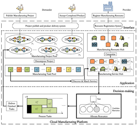
Figure 1.
Architecture of the Cloud Manufacturing platform.

Table 1.
Nomenclature.
This architecture is mainly composed of three layers of functions, namely interface, application, and decision-making. The real-time scheduling problem comes from the decision-making layer. Accordingly, the process of the demander using the services provided by the platform can be described as follows:
- Demanders publish MP (Manufacturing Project) to the platform;
- Platform decomposes MP into MTs (Manufacturing Tasks);
- Platform discovers and matches MR (Manufacturing Resource) in type-matched MS (Manufacturing Service) for these MTs;
- Platform allocates MR for the processing of MT.
- Providers arrange MTs using professional software and deliver the completed MTs to demanders.
Therefore, the scheduling problem in the CMfg environment is as follows: how to reasonably allocate the emerging MTs to the type-matched MRs in real-time under the constraints of task precedence, resource occupation, and logistics duration while reducing the service costs, improving the service quality, and shortening the make-span for each MP?
Since the scheduling environment of CMfg is larger and more dynamic than that of the traditional workshop [17,18], it is much more difficult to find the optimal solution. As a consequence, the focus of related research turns to find the approximate optimal solution. As a major branch of approximation methods, a search-based heuristic scheduling approach expands the current schedule with well-designed strategies. The keys to designing such an approach are the neighborhood structure and the search direction, such as Simulated Annealing, Tabu-search, Discrete Search, Genetic Algorithm, and so on [19,20,21,22,23]. However, these algorithms cannot be directly applied to the scheduling problem in the CMfg environment because they will take a long time for the solution searching.
In order to solve the real-time scheduling problem, researchers have proposed and developed numerous approaches and algorithms that can be divided into two categories: generative and adaptive. Generative scheduling adopts the idea of integrating partial-schedules, and the key lies in the design of priority rules. However, the priority rules for the determined manufacturing environment are not suitable for dynamic random situations [24]. Hence, adaptive methods have attracted more researchers. Adaptive scheduling, which is also called rescheduling, modifies the existing schedule dynamically according to the decision environment. Proactive and reactive are the two main modes of rescheduling [25]. Due to the uncertain factors, such as task delay, unit failure, and order insertion, the disturbances become difficult to predict, which means that the proactive rescheduling cannot be used in the real-time environments [26]. As a result, more and more researchers have begun to focus on reactive or hybrid rescheduling methods [27]. One group studied the random resource constrained project scheduling problem. They transformed the problem into a multi-stage decision problem, and made dynamic decisions by designing rescheduling strategies [28]. Another group studied the rescheduling problem with new operation insertion in a single machine environment. They set up an event-triggered rescheduling model with the goal of minimizing the absolute deviation of the maximum delay compared with the baseline [29]. For the dynamic manufacturing environment where tasks arrive randomly, a dynamic event-driven task rescheduling method is designed to avoid service rearrangement, and the constructed parallel processing strategy takes service time, logistics time, the earliest available time, and other factors into consideration at the same time for optimal service selection [30]. Researchers have also proposed two reactive scheduling strategies based on the selection and buffering to solve the random resource constrained project scheduling problem. They found that the buffer-based reaction rules combined with the baseline scheduling turned out to be an effective solution [31].
The above reviews indicate that it is difficult to efficiently allocate massive manufacturing resources in the CMfg environment for the real-time scheduling. Research on the real-time scheduling in the CMfg is scarce, and the proposed scheduling methods are based on reactive scheduling strategy, the baseline of which is set in advance and needs to be modified as the environment changes. For the dynamic CMfg environment, such scheduling methods will consume numerous computing resources. Changing schedules often results in the re-allocation of resources, which will lead to additional logistics costs. Generally, real-time scheduling using these approaches requires a trade-off between the solution quality and decision efficiency. With the development of artificial intelligence, more and more teams are trying to apply related technologies to the manufacturing scope [32]. In order to solve the scheduling problem in the manufacturing environment, many neural networks are used to determine the key parameters to improve the performance of the genetic algorithm [33,34].
In this paper, we convert the aforementioned scheduling problem into the form of estimating the optimal objective value, and an ANN-based model is established to predict the task completion status for each candidate resource as the principle for allocating manufacturing tasks. The trained ANN model has high prediction accuracy, and the proposed ANN-based approach performs well in terms of the optimization objectives, including cost, satisfaction, and make-span. The high responsiveness of the ANN-based approach makes it suitable for the real-time scheduling in the CMfg environment.
The structure of the paper is as follows. First, we establish a mathematical model of the real-time scheduling problem in the CMfg environment in Section 2. Then, the solution framework of this problem is defined in Section 3. As the key issue in this framework, the decision of task allocation is made using a trained ANN model. Section 4 conducts comparison experiments for scheduling methods in terms of objectives and responsiveness. The application design for the proposed ANN-based approach is depicted in Section 5. Section 6 presents the conclusion.
2. Mathematical Modeling for the CMfg Scheduling Problem
According to the CMfg platform architecture (Figure 1), the real-time scheduling can be described as the procedure shown in Figure 2.
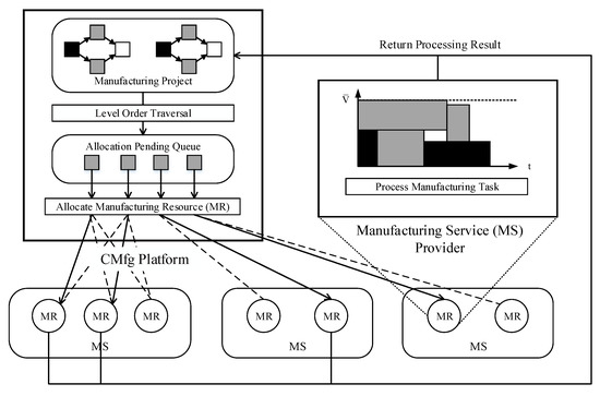
Figure 2.
Real-time Schedule Procedure in the Cloud Manufacturing (CMfg) Environment.
The MPs in the CMfg platform consist of MTs with precedence sequence, the waiting ones for allocation are in white, and the ones in allocating are filled in gray, while the completed ones are filled in black. By using level-order traversal, the operator can allocate MTs to the type-matched MRs without precedence constraints, and these tasks will be manufactured by the corresponding providers.
Basic assumptions, as follows, are needed to focus on our research scope before mathematical modeling:
- The set-up time for MT is already included in the processing time;
- No interruption is considered in the processing of MTs;
- The capacity of MR occupied by task processing will be released when the processing is completed;
- Transportation logistics need to be considered before and after the processing of MT.
2.1. Formal Expression of the Main Components
The main components of the CMfg environment are MT and MR. Due to the consideration of management granularity, these two components are not directly presented to the scheduling problem.
Providers distributed in different locations register their encapsulated and virtualized MR capabilities to the CMfg platform. Then, the platform operator classifies these MRs according to their capability types and abstracts them into MS, which is an integrated form of MRs for the demander to use. Specifically, MS of type k can be expressed by a tuple, as shown in Equation (1).
where represents the label set of MR in the same type, and denotes the allocation pending queue of MTs at time t.
For MR labeled i in , its attributes are expressed as Equation (2).
where and represent unit cost and service quality, respectively. is the maximum available capacity at time t, and is its upper bound. and denote the processing pending queue of MTs and the active MT set defined in Equation (3) at time t, respectively.
where is the label mark of MT, and , respectively, represent the start time and finish time of processing this MT. Symbol is a 0–1 decision variable defined as Equation (4).
In the cloud platform, MP that is published by the demander will be pooled, and the precedence relationship of the contained MTs can be described as the activity-on-vertex network, as shown in Figure 3.
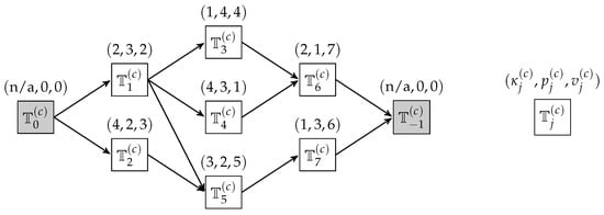
Figure 3.
Activity-on-Vertex of Manufacturing Project (MP) (n/a means not applicable).
Where and are dummy MTs to help stylize the MP into a single-input-single-output graph. Specifically, an MP labelled c can be expressed by a tuple shown in Equation (5).
where represents the label set of MT included in , denotes the publish time, and is the logistics duration vector defined as Equation (6).
where is the logistics duration between and .
For MT labelled j in , its attributes can be represented as Equation (7).
where , , and represent required service capacity, service capability type, and processing time, respectively. and , respectively, denote the immediate predecessor and the successor set.
In this way, the mathematical model of real-time scheduling in the CMfg environment can be expressed as Equations (8)–(16), and it is a multi-objectives optimization problem.
where denotes the set of arrived MPs during time interval , and the objective function of Equation (8) is the accumulated mean value of objective vector defined as Equation (9). The composition of the objectives and the Constraints (10)–(16) will be described in detail in the rest of this section.
2.2. Optimization Objectives for Real-Time Scheduling
For each MP, the scheduling optimization objectives include three aspects, namely cost, make-span, and service quality. Without loss of generality, we proceed from the perspective of .
First of all, the service usage cost for any MP is incurred when the demander requests and uses specific MRs included in the type-matched MSs, it is equal to the sum of the usage costs of MTs inside the MP. The service usage cost for MT is determined by the unit cost of the allocated MR and the requirement for task processing. Specifically, if is allocated to for processing, the service usage cost is determined by Equation (17).
Then, the service usage cost for will be Equation (18)
Secondly, the make-span of MP refers to the overall processing time to complete all its MTs. It needs to consider the logistics duration for all the MTs inside the MP. According to the activity-on-vertex of as shown in Figure 3, its make-span can be expressed as Equation (19), where belongs to dummy .
Thirdly, the quality of the product refers to the satisfaction of manufacturing , and it is determined by the intrinsic service quality of specific MRs. Since the satisfaction of processing can be expressed as Equation (20), the quality of the product for processing can be defined as Equation (21), which is the lowest satisfaction obtained by processing MTs included in .
2.3. Constraints for Real-Time Scheduling
Constraints for real-time scheduling problems in the CMfg environment include task precedence, resources occupation, logistics duration, and so on.
Specifically, Constraints (10) and (11) indicate the logical limitation of allocation, which means that for type-matched MRs, any MT can only be assigned to one of them for processing, and each of the MT can only be processed once. As formulated in Equation (12), the processing time of any MT needs to be guaranteed, that is, the time span between the start time and the finish time of processing is at least equal to the required processing time .
During the processing of MT, Equation (13) means the available capacity of MR needs to be no less than the capacity required by the MT, and Equation (14) indicates the sum of occupied capacity by active MTs does not exceed the maximum resource capacity at time t. Take , for example, as shown in Figure 4, the capacity upper bound is , and the rectangle in black indicates the resource occupation of the provider’s internal planning task. At time , the maximum available capacity of becomes , so it is reasonable to manufacture () and () at this time slot since the sum of occupied capacity does not exceed (); hence, we get the active MT set as .
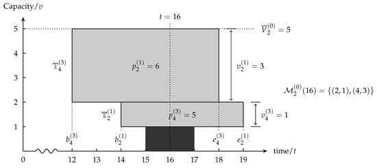
Figure 4.
Capacity occupation of , checking at .
Figure 5 depicts the precedence constraints in MP that contain Equations (15) and (16), which, respectively, mean the ready time of any MT is no earlier than the complete time of its predecessors and the start time of any MT is no earlier than its ready time plus its logistics duration.
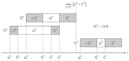
Figure 5.
Precedence constraint of with logistics duration considered.
Where the auxiliary variable is defined as Equation (22).
3. Artificial Neural Network based Resource Allocation Methodology
The main purpose of the real-time scheduling problem is to allocate MSs for every MT, and the allocation of can be depicted as Figure 6. The candidate MRs are determined by their capability type and the upper bound of available capacity as formulated in Equation (23).
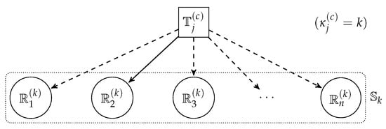
Figure 6.
Allocating to one of the candidate MRs in , the capability type is matched.
However, since the number of candidate MRs is large and the processing statuses of these MRs are changing over time, the conventional search algorithms are no longer applicable because they will spend a long time checking all of the possible time intervals in every candidate MR. Therefore, we adopt an ANN that is based on the multi-layer perceptron architecture to speed up the searching procedure by estimating the objective values of each candidate MR.
Specifically, take as an example, after filtering out candidate MRs according to (23), the objective values projected on MT can be estimated by the completion status prediction model as shown in Figure 7.
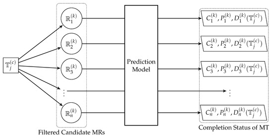
Figure 7.
Procedure of Manufacturing Task (MT) completion status prediction on candidate Manufacturing Resources (MRs.)
Since both and are intrinsic values of , the key of this prediction model is to predict the completion time of . It can be known from the activity-on-vertex structure of one MP (Figure 3), that is, one MT will affect the make-span of its MP only if it is on the critical path, otherwise it has a flexible interval for completion time. Using the level-order traversal algorithm, the upper and lower bounds of the ideal completion time of that may not affect the make-span of its MP can be obtained. Then, the upper and lower bounds can divide the time axis into three adjacent sections, and their probabilities are Equations (24)–(26).
where means the probability of completion time lies in time interval “Completion status n”. Since the completion status of can only belong to one of these three statuses, we have . Then the allocation preference for MR candidates of can be defined as Equation (27), which motivates the allocation of MR to process as early as possible.
As shown in Figure 8, the ANN predicts the completion status of MT.
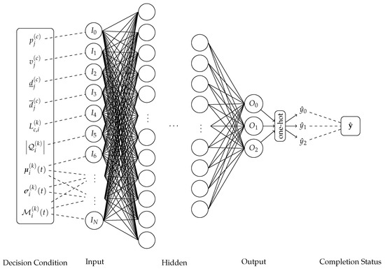
Figure 8.
Artificial Neural Network model for the MT completion status prediction.
Where , , represent , , , respectively. The expression of actual completion status of processed on is defined as Equation (28).
The inputs of this ANN are written in Input (29), which means all the possible features from the decision condition.
The decision condition for allocated to consists of intrinsic attributes of (, , , , ) and dynamic features of defined in Equation (30).
where and are the mean value and standard deviation value of the processing pending queue at time t, respectively.
4. Numerical Results
4.1. Experimental Environment Setting
We conduct comparative experiments to verify the effectiveness of the proposed ANN-based approach for real-time scheduling, and the dataset is adapted from MPSPLib (www.mpsplib.com/download.php), which consists of multiple project instances defined in Table 2.
Table 2.
Project Instance in MPSPLib (take file j301_1.sm as an example).
According to the MT scale of projects in the aforementioned MPSPLib, the experimental dataset is grouped as follows:
- Exp-30
- Each MP in this group contains 30 MTs;
- Exp-60
- Each MP in this group contains 60 MTs;
- Exp-90
- Each MP in this group contains 90 MTs;
- Exp-120
- Each MP in this group contains 120 MTs;
- Exp-mix
- MT scale of each MP in this group can be any value in .
Each project in the MPSPLib is enabled with random features as Equations (33)–(37) to imitate the process of publishing MPs to the CMfg platform from the demanders and to enlarge the diversity of MS from the providers.
where represents a random distribution over the interval , and the involved parameters are listed in Table 3.
Table 3.
Parameters for MP and MS in the experimental environment.
4.2. Preparation for Real-Time ANN-Based Scheduling Approach
The network inside the ANN-based approach is constructed in PyTorch, and its main parameters are listed in Table 4.
Table 4.
Parameters for the training of the Artificial Neural Network (ANN).
Before starting to train the ANN model, we need to sample the data that is consistent with the style of Input (29) and Output (31). The quality of an ANN model can be judged by its cross-entropy loss function in Equation (38) during training, as depicted in Figure 9.
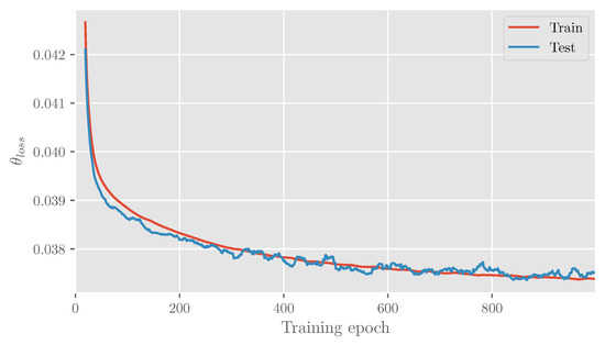
Figure 9.
Cross-entropy loss of train/test dataset over 1000 training epochs.
As shown in Figure 9, after 1000 epochs, the training loss and testing loss both reached a small range and gradually converged. As the number of training epoch increases, the difference between training loss and testing loss becomes smaller and smaller, which indicates that the proposed ANN-based approach has the ability for generalization. Figure 10 plots the prediction accuracy as Equation (39) to evaluate the performance of the ANN model.
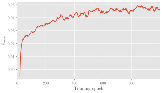
Figure 10.
Prediction accuracy of the ANN model over 1000 training epochs.
After 1000 iterations, the prediction accuracy on the test set gradually converges to a high region about , and other evaluation metrics are listed in Table 5. These metric values demonstrate the effectiveness of the ANN-based completion status prediction model.
Table 5.
Conventional evaluation metrics for the ANN.
4.3. Performance with Discussions
We use the modified NSGA-II (Nondominated Sorting Genetic Algorithm version II) [35] as the referred method for the comparative experiment. Specifically, the corresponding modification is based on the approximation that the whole problem is divided into the time dimension initially, then NSGA-II() is called to solve the divided sub-problems one by one. The problem segmentation factor indicates the degree of the division, that means no division and will mimic the effect of real-time scheduling. Figure 11a–e show the performance comparison of these methods in terms of total cost, service satisfaction, and make-span.
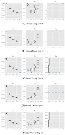
Figure 11.
Performance comparison on various MT Scales, () represents NSGA-II() in the x-labels, .
Since the dataset groups for these experiments mentioned in Section 4.1 are dimensionless quantities, we use comparison ration in Equation (40) to evaluate the performance of the scheduling methods.
where means the average of the objective value gained by the corresponding method, and the summarized experimental results are listed in Table 6.
Table 6.
Summarized objective values result from different scheduling methods.
In each group of the dataset, the ANN-based method has an absolute advantage in the cost () compared to the NSGA-II() method series. Although the advantages of ANN in make-span () and service satisfaction () are not significant, this method has also reached higher levels in both criteria. For the NSGA-II() method series, as the value of division factor increases, the number of sub-problems decreases, which leads to the decrease of cost, but the make-span increases. As for the service satisfaction, all of the methods perform similarly, which are mainly due to the limited number of candidate MRs in each MS. It can be inferred that the ANN-based approach has a strong generalization ability since it has a great performance in different dataset groups.
In addition to the objective values, another important indicator is the responsiveness that measures the decision time of each allocation procedure in the scheduling. Figure 12 summarizes the average responsiveness for each dataset group, the decision time for using the ANN to determine a schedule is only about of the NSGA-II() on average.
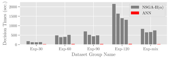
Figure 12.
Average Responsiveness of NSGA-II() series and ANN.
As for the performance of the ANN-based approach on a single MR allocation for each MT, Table 7 summarizes the average decision time.
Table 7.
Average decision time of the ANN-based approach.
The average decision time for MR allocation is under 50 ms, and the average decision time for determining a schedule is under 40s, which indicates that the ANN-based approach is suitable for the real-time scheduling because, compared to the NSGA-II, the proposed ANN-based approach only takes of the decision time to determine a sound schedule in such a discrete manufacturing environment, and the decision time is negligible if compared to the duration of resource configuration, manufacturing execution, transportation, and so on, which are usually measured in hours or days.
5. Application Design of ANN-Based Real-Time Scheduling in the Cloud Manufacturing Environment
Mold casting is a common industry that applies the CMfg. Figure 13 shows its demand and supply distribution in the Zhejiang province.
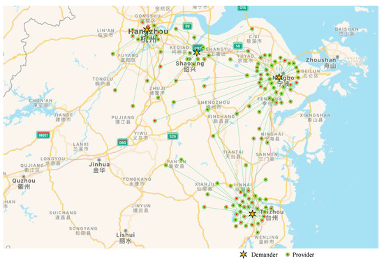
Figure 13.
Provider and demander distribution in the CMfg environment.
It can be seen that the demanders are surrounded by numerous providers, and the resource optimization and coordination are in desperate need. With the increase in diversity and complexity of requirements from demanders, the real-time scheduling becomes much more difficult. Figure 14 shows the procedure for the demander to use MR via the CMfg platform.
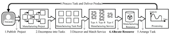
Figure 14.
Procedure for demander to use MR via the CMfg platfrom.
The key step is the allocation of MR, which can be realized by the ANN. Figure 15 shows the functional design of the application of the proposed ANN-based approach in the CMfg environment.
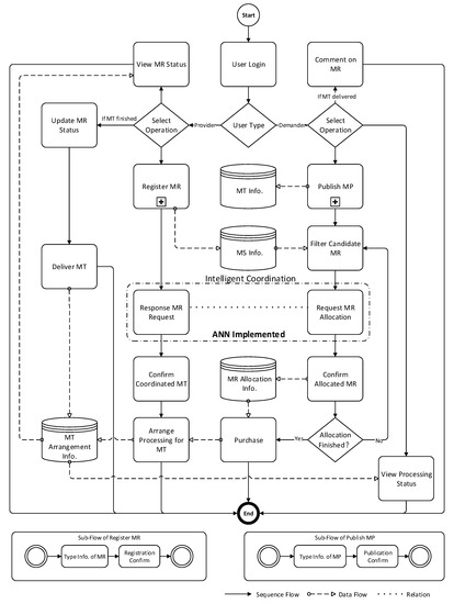
Figure 15.
Logical flow chart of application design of ANN-based scheduling in the CMfg environment.
The “Intelligent coordination” module that implements the ANN will handle the real-time scheduling problem, and putting the design into practical application is an ongoing work.
6. Conclusions
In this paper, we studied the real-time scheduling problem in the CMfg environment. After presenting the premises and antecedents, several research contents and the results can be pointed out:
- We constructed a mathematical model for real-time scheduling in the CMfg environment with optimization objectives as minimizing the cost, minimizing the make-span, and maximizing the service satisfaction constrained by task precedence, resource occupation, and logistics duration;
- An ANN-based approach for real-time scheduling has been designed, it uses the MT attributes and process pending queue of MR as inputs to predict the completion status of MT if it will be allocated to any of the candidate MRs;
- We conducted the comparison experiments and modified the NSGA-II as the referred scheduling method, the results show that:
- The proposed ANN-based approach performs better than the NSGA-II in terms of objective values;
- The response time of the ANN is only about of the NSGA-II on average;
- Using ANN, the average decision time for MR allocation is under 50 ms, which indicates that the proposed ANN-based approach is suitable for the real-time scheduling.
- We designed the application of ANN-based real-time scheduling to show how to implement this method to help coordinate providers of MR in the CMfg environment.
In addition, the proposed method has good performances on different MT scale datasets, which indicates its generalization ability. Since the proposed ANN-based approach solves the common problem for the platform based manufacturing environment, it can also be used in related web based manufacturing environments.
It should be noticed that the research in this article is mainly based on the library instances rather than the data from the real-world. Since there is no exactly the same real-time scheduling problem as described in this paper, the proposed ANN-based approach is not compared with other articles which also use ANN model to prove we have a better result. How to improve the ANN of the proposed real-time scheduling approach to perform better and apply this approach to the real world is our on-going work.
Author Contributions
Conceptualization, S.C. and S.F.; formal analysis, S.C.; funding acquisition, S.F.; methodology, S.C.; project administration, S.F. and R.T.; validation, S.C.; writing—original draft, S.C.; writing—review and editing, S.F. and R.T. All authors have read and agreed to the published version of the manuscript.
Funding
This research was funded by 1. National Natural Science Foundation of China (grant number 71571161); 2. National High-tech Research and Development Program (grant number 2015AA042101); 3. Science Fund for Creative Research Groups of National Natural Science Foundation of China (grant number 51821093).
Conflicts of Interest
The authors declare no conflict of interest.
References
- Zhou, K.; Liu, T.; Zhou, L. Industry 4.0: Towards Future Industrial Opportunities and Challenges. In Proceedings of the 12th International Conference on Fuzzy Systems and Knowledge Discovery (FSKD), Zhangjiajie, China, 15–17 August 2015; pp. 2147–2152. [Google Scholar] [CrossRef]
- Li, P.; Jiang, P.; Liu, J. Mini-MES: A Microservices-Based Apps System for Data Interconnecting and Production Controlling in Decentralized Manufacturing. Appl. Sci. 2019, 9, 3675. [Google Scholar] [CrossRef]
- Qu, Y.J.; Ming, X.G.; Liu, Z.W.; Zhang, X.Y.; Hou, Z.T. Smart Manufacturing Systems: State of the Art and Future Trends. Int. J. Adv. Manuf. Technol. 2019, 103, 3751–3768. [Google Scholar] [CrossRef]
- He, W.; Xu, L. A State-of-the-Art Survey of Cloud Manufacturing. Int. J. Comput. Integr. Manuf. 2015, 28, 239–250. [Google Scholar] [CrossRef]
- Adamson, G.; Wang, L.; Holm, M.; Moore, P. Cloud Manufacturing—A Critical Review of Recent Development and Future Trends. Int. J. Comput. Integr. Manuf. 2017, 30, 347–380. [Google Scholar] [CrossRef]
- Prinsloo, J.; Sinha, S.; von Solms, B. A Review of Industry 4.0 Manufacturing Process Security Risks. Appl. Sci. 2019, 9, 5105. [Google Scholar] [CrossRef]
- Nazarenko, A.A.; Sarraipa, J.; Camarinha-Matos, L.M.; Garcia, O.; Jardim-Goncalves, R. Semantic Data Management for a Virtual Factory Collaborative Environment. Appl. Sci. 2019, 9, 4936. [Google Scholar] [CrossRef]
- Liu, Y.; Xu, X. Industry 4.0 and Cloud Manufacturing: A Comparative Analysis. J. Manuf. Sci. Eng. 2017, 139, 034701. [Google Scholar] [CrossRef]
- Tran, N.H.; Park, H.S.; Nguyen, Q.V.; Hoang, T.D. Development of a Smart Cyber-Physical Manufacturing System in the Industry 4.0 Context. Appl. Sci. 2019, 9, 3325. [Google Scholar] [CrossRef]
- Ren, L.; Zhang, L.; Wang, L.; Tao, F.; Chai, X. Cloud Manufacturing: Key Characteristics and Applications. Int. J. Comput. Integr. Manuf. 2017, 30, 501–515. [Google Scholar] [CrossRef]
- Tran, L.V.; Huynh, B.H.; Akhtar, H. Ant Colony Optimization Algorithm for Maintenance, Repair and Overhaul Scheduling Optimization in the Context of Industrie 4.0. Appl. Sci. 2019, 9, 4815. [Google Scholar] [CrossRef]
- Behnamian, J. Heterogeneous Networked Cooperative Scheduling With Anarchic Particle Swarm Optimization. IEEE Trans. Eng. Manag. 2017, 64, 166–178. [Google Scholar] [CrossRef]
- Moghaddam, M.; Nof, S.Y. Collaborative Service-Component Integration in Cloud Manufacturing. Int. J. Prod. Res. 2018, 56, 677–691. [Google Scholar] [CrossRef]
- Díaz-Reza, J.R.; Mendoza-Fong, J.R.; Blanco-Fernández, J.; Marmolejo-Saucedo, J.A.; García-Alcaraz, J.L. The Role of Advanced Manufacturing Technologies in Production Process Performance: A Causal Model. Appl. Sci. 2019, 9, 3741. [Google Scholar] [CrossRef]
- Xu, X. From Cloud Computing to Cloud Manufacturing. Robot. Comput.-Integr. Manuf. 2012, 28, 75–86. [Google Scholar] [CrossRef]
- Wu, D.; Greer, M.J.; Rosen, D.W.; Schaefer, D. Cloud Manufacturing: Strategic Vision and State-of-the-Art. J. Manuf. Syst. 2013, 32, 564–579. [Google Scholar] [CrossRef]
- Yang, G.; Chung, B.D.; Lee, S.J. Limited Search Space-Based Algorithm for Dual Resource Constrained Scheduling Problem with Multilevel Product Structure. Appl. Sci. 2019, 9, 4005. [Google Scholar] [CrossRef]
- Choi, Y.B.; Yun, H.Y.; yeop Kim, J.; Jin, S.H.; Kim, K.S. Robust Optimization Approach Using Scenario Concepts for Artillery Firing Scheduling Under Uncertainty. Appl. Sci. 2019, 9, 2811. [Google Scholar] [CrossRef]
- Boctor, F.F. Resource-Constrained Project Scheduling by Simulated Annealing. Int. J. Prod. Res. 1996, 34, 2335–2351. [Google Scholar] [CrossRef]
- Nonobe, K.; Ibaraki, T. Formulation and Tabu Search Algorithm for the Resource Constrained Project Scheduling Problem. In Essays and Surveys in Metaheuristics; Ribeiro, C.C., Hansen, P., Eds.; Operations Research/Computer Science Interfaces Series; Springer: Boston, MA, USA, 2002; pp. 557–588. [Google Scholar]
- Bouleimen, K.; Lecocq, H. A New Efficient Simulated Annealing Algorithm for the Resource-Constrained Project Scheduling Problem and Its Multiple Mode Version. Eur. J. Oper. Res. 2003, 149, 268–281. [Google Scholar] [CrossRef]
- Mahdi Mobini, M.D.; Rabbani, M.; Amalnik, M.S.; Razmi, J.; Rahimi-Vahed, A.R. Using an Enhanced Scatter Search Algorithm for a Resource-Constrained Project Scheduling Problem. Soft Comput. 2009, 13, 597–610. [Google Scholar] [CrossRef]
- Zamani, R. A Competitive Magnet-Based Genetic Algorithm for Solving the Resource-Constrained Project Scheduling Problem. Eur. J. Oper. Res. 2013, 229, 552–559. [Google Scholar] [CrossRef]
- Chen, Z.; Demeulemeester, E.; Bai, S.; Guo, Y. Efficient Priority Rules for the Stochastic Resource-Constrained Project Scheduling Problem. Eur. J. Oper. Res. 2018, 270, 957–967. [Google Scholar] [CrossRef]
- Vieira, G.E.; Herrmann, J.W.; Lin, E. Rescheduling Manufacturing Systems: A Framework of Strategies, Policies, and Methods. J. Sched. 2003, 6, 39–62. [Google Scholar] [CrossRef]
- Lamas, P.; Demeulemeester, E. A Purely Proactive Scheduling Procedure for the Resource-Constrained Project Scheduling Problem with Stochastic Activity Durations. J. Sched. 2016, 19, 409–428. [Google Scholar] [CrossRef]
- Davari, M.; Demeulemeester, E. The Proactive and Reactive Resource-Constrained Project Scheduling Problem. J. Sched. 2019, 22, 211–237. [Google Scholar] [CrossRef]
- Herroelen, W.; Leus, R. Robust and Reactive Project Scheduling: A Review and Classification of Procedures. Int. J. Prod. Res. 2004, 42, 1599–1620. [Google Scholar] [CrossRef]
- Akkan, C. Improving Schedule Stability in Single-Machine Rescheduling for New Operation Insertion. Comput. Oper. Res. 2015, 64, 198–209. [Google Scholar] [CrossRef]
- Zhou, L.; Zhang, L.; Sarker, B.R.; Laili, Y.; Ren, L. An Event-Triggered Dynamic Scheduling Method for Randomly Arriving Tasks in Cloud Manufacturing. Int. J. Comput. Integr. Manuf. 2018, 31, 318–333. [Google Scholar] [CrossRef]
- Davari, M.; Demeulemeester, E. Important Classes of Reactions for the Proactive and Reactive Resource-Constrained Project Scheduling Problem. Ann. Oper. Res. 2019, 274, 187–210. [Google Scholar] [CrossRef]
- Arnaiz-González, Á.; Fernández-Valdivielso, A.; Bustillo, A.; López de Lacalle, L.N. Using Artificial Neural Networks for the Prediction of Dimensional Error on Inclined Surfaces Manufactured by Ball-End Milling. Int. J. Adv. Manuf. Technol. 2016, 83, 847–859. [Google Scholar] [CrossRef]
- Yuce, B.; Rezgui, Y.; Mourshed, M. ANN–GA Smart Appliance Scheduling for Optimised Energy Management in the Domestic Sector. Energy Build. 2016, 111, 311–325. [Google Scholar] [CrossRef]
- Wang, L.; Guo, C.; Li, Y.; Du, B.; Guo, S. An Outsourcing Service Selection Method Using ANN and SFLA Algorithms for Cement Equipment Manufacturing Enterprises in Cloud Manufacturing. J. Ambient Intell. Hum. Comput. 2019, 10, 1065–1079. [Google Scholar] [CrossRef]
- Deb, K.; Pratap, A.; Agarwal, S.; Meyarivan, T. A Fast and Elitist Multiobjective Genetic Algorithm: NSGA-II. IEEE Trans. Evol. Comput. 2002, 6, 182–197. [Google Scholar] [CrossRef]


© 2020 by the authors. Licensee MDPI, Basel, Switzerland. This article is an open access article distributed under the terms and conditions of the Creative Commons Attribution (CC BY) license (http://creativecommons.org/licenses/by/4.0/).