Article

Segmentation of River Scenes Based on Water Surface Reflection Mechanism

State Key Laboratory of Industrial Control Technology, College of Control Science and Engineering, Zhejiang University, Hangzhou 310027, China
*
Author to whom correspondence should be addressed.
Appl. Sci. 2020, 10(7), 2471; https://doi.org/10.3390/app10072471
Submission received: 15 February 2020 / Revised: 29 March 2020 / Accepted: 30 March 2020 / Published: 3 April 2020
(This article belongs to the Special Issue Texture and Colour in Image Analysis)

Abstract

:
Segmentation of a river scene is a representative case of complex image segmentation. Different from road segmentation, river scenes often have unstructured boundaries and contain complex light and shadow on the water’s surface. According to the imaging mechanism of water pixels, this paper designed a water description feature based on a multi-block local binary pattern (MB-LBP) and Hue variance in HSI color space to detect the water region in the image. The improved Local Binary Pattern (LBP) feature was used to recognize the water region and the local texture descriptor in HSI color space using Hue variance was used to detect the shadow area of the river surface. Tested on two data sets including simple and complex river scenes, the proposed method has better segmentation performance and consumes less time than those of two other widely used methods.

1. Introduction

Segmentation of a river scene plays an important role in many fields such as the water hazard detection of unmanned ground vehicles [1], the navigation of unmanned ships [2], river analysis or flood monitoring by remote sensing [3,4,5,6] and vision-based object monitoring on rivers. This study aims to recognize the river region in an image taken in outdoor scenes based on the water surface reflection mechanism, which is an important task in applications of intelligent video surveillance in river environments. Moreover, segmentation of the river scene is a representative case of complex image segmentation, which can serve as a reference for complex image segmentation.
For water region segmentation, researchers have explored different kinds of methods that fall into three main categories—image processing-based methods, Machine Learning-based methods (including Deep Learning, Supervised Learning, Clustering, etc.), and hardware-based methods. For image processing-based methods, Rankin et al. [7] combined the color and texture features to detect the water region according to the appearance characteristics of the river in the outdoor scene. Yao [8] used the Region Growing method firstly to separate the obvious water region based on the brightness value. Then a designed texture feature is used to perform K-Means clustering on each 9 × 9 small patch in the image, where the class with the smallest average value of texture is classified as the water region, where the detection of water region with shadow needs the aid of stereo vision. Zhao et al. [9] used the adaptive threshold Canny edge detection algorithm to detect the river boundary. The texture and structure of images are also widely used in related research in water scenes such as waterline detection [10] and maritime horizon line detection [11]. For Machine Learning-based methods, Achar et al. [12] proposed a self-supervised algorithm to classify all the image patches in an image into water or not-water category by features of RGB, texture, and height. The results show high accuracy but this algorithm requires prior knowledge of horizon by hardware and is only applicable to images that conform to a specific structure. Moreover, with the development of Deep Learning, it has also been applied in water region segmentation. For example, Zhan et al. [13] proposed an online learning approach to recognize the water region for the USV in the unknown navigation environment using a convolutional neural network (CNN). Han et al. [14] innovatively used the Fully Connected Convolutional Network (FCN) to achieve water hazards detection on the road. Despite of high accuracy, the artificial neural network with complex structure needs to be pre-trained in many scenes before use and requires high computing power. For hardware-based methods, some studies have used various optical sensors such as laser radar [15], infrared camera [1], stereo camera [16,17], and polarized camera [16,18,19] to easily realize water hazard detection based on the optical characteristics of waters [20]. These methods are still difficult to popularize in applications due to the cost and equipment complexity.
The above methods have some defects. As Rankin [21] made the observation that the river has inhomogeneous appearance in outdoor scenes, the methods simply utilizing image features, whose underlying assumption is that river appearance is fairly uniform, remain problematic due to inhomogeneous appearance (such as shadow and changing illumination) and show bad performance. For the same reason, it is also inappropriate for Machine Learning-based methods using the global features of an image to train a classification model to segment itself. As for the hardware-based methods, they are beyond the scope of this paper.
Since image processing technology has advantages of simplicity and interpretability, this study proposes a segmentation algorithm utilizing designed image features without machine learning. To overcome the drawback that the current methods cannot well deal with inhomogeneous appearance of the river, this study designs an improved LBP feature extraction method based on the water surface reflection mechanism to detect water region in the image. A texture feature based on Hue(H) variance in HSI color space is also introduced for detection of shadow area. Compared with two other principle methods using image processing techniques, the proposed method consumes the least time, and in the complex river scenes where other methods failed, the proposed algorithm still shows satisfactory performance. Lastly in this study, the parameters in the proposed algorithm are discussed for better performance.

2. Materials and Methods

2.1. Algorithm Framework

The qualitative imaging law of the riverine water region in an image is the basis of the algorithm designed in this paper. The overall flowchart of the proposed algorithm is shown in Figure 1.
First of all, the input image needs to be pre-processed, including image down-sampling and image blurring operation. The pre-processing operations will be discussed in Section 3.1. Secondly, the improved LBP feature and local hue variance are calculated in parallel. Then the water region with and without shadow are both obtained by threshold method. The two parts are fused as the major water region. Finally, the image morphological operation is carried out on the candidate region of the water region. After obtaining the results of the morphological processing, the largest connected domain is taken as the final water region. Judging the maximum connected domain is also an important task. It is based on the common sense that the water area often occupies a main and large part of the image, which helps to eliminate the pseudo-water patches whose features are similar to those of water patches.

2.2. Light Reflection Mechanism of Water Surface

In order to study the imaging law of water in rivers, it is necessary to first understand the general reflection mechanism of objects. According to Lambert Law, the intensity of object surface through various types of reflections reaches the image sensor is [22]:
I ( x ) = ω e ( λ ) ρ k s ( x , λ ) d λ ,
where e ( λ ) is the color of the light source, s ( x , λ ) is the surface reflection value, ρ k is the sensitive function of the camera ( k { R , G , B } ), ω represents the visible spectral range, and x denotes the corresponding space coordinates. For a particular color camera, the pixel intensity values in the image are only related to the reflected light [23]. On this basis, the relationship between the pixel value of the water and the light reflection of the water surface is further expressed as follows:
I = L R total ,
where L is the illumination factor related to the illumination condition, R total is the total reflection energy. In river scenes, R total is mainly composed of the following four parts [21]: the energy that reflected off the water surface R r , that scattered by water molecules to the camera R o , that reflected or scattered by materials suspended in the water to the camera R s , and that reflected off the bottom of the water the camera R p :
R total = R r + R o + R s + R p .
Since the reflection from the water surface to the camera R r plays a dominant role in R total , that is, (2) and (3) can be further simplified as:
I L R r .
For light polarized perpendicular to and parallel to the plane of incidence, R r can be respectively decomposed into R r , ( θ ) and R r , ( θ ) , where θ is the incident angle, θ 0 , π 2 , as shown in (5):
R r ( θ ) = R r , ( θ ) + R r , ( θ ) 2 .
According to Fresnel Law:
R r , ( θ ) = [ n 1 cos θ n 2 1 n 1 n 2 sin θ 2 n 1 cos θ + n 2 1 n 1 n 2 sin θ 2 ] 2 ,
R r , ( θ ) = [ n 1 1 n 1 n 2 sin θ 2 n 2 cos θ n 1 1 n 1 n 2 sin θ 2 + n 2 cos θ ] 2 ,
where n 1 is the refractive index of air, n 2 is the refractive index of water, and θ is the angle of incidence. n 1 = 1.0 and n 2 = 1.33 are taken under ideal conditions.The water region reaches the sensor through various types of reflections, as shown in Figure 2, where l is the horizontal displacement of the point to the camera lens, h is the height at which the camera is placed (in a certain scene, the image sensor used to capture images is commonly fixed). According to the simplified scenario shown in Figure 2, α θ can be obtained from the geometric relationship, thus R r ( θ ) can be converted into a function R r ( l ) about the horizontal displacement, just make:
θ arctan l h
and then substitute (8) into (5). Since only qualitative rather than quantitative law is used in the subsequent algorithm design for the water region detection, the above equation do not need to be strictly equal. Given that the expression of the result is too complicated, and the designed algorithm only needs the qualitative law, we explored the relationship between the reflection intensity of the water and the horizontal distance to the camera by giving some different h values that indicate some conventional installation heights, as shown in Figure 3.
It can be seen that the reflected energy to the image sensor from far to near is monotonically decreasing. This qualitative law of water pixels is used to design subsequent water region detection algorithm.
In addition to the above-mentioned reflection mechanism, the water surface in outdoor scenes often contains shadow caused by the occlusion of the riverside scenery. The H component in the HSI color space of the image is not sensitive to illumination, and can maintain a relatively stable state under illumination changes [24]. In order to calculate the feature of H, firstly the RGB image should be converted into an HSI one by:
h = β , g b 2 π β , g < b , h [ 0 , 2 π ]
s = 1 3 · min ( r , g , b ) , s [ 0 , 1 ]
i = r + g + b 3 , i [ 0 , 1 ] ,
where r, g, b, h, s, i are all normalized values, and:
β = arccos [ ( r g ) + ( r b ) ] / 2 ( r g ) 2 + ( r b ) ( g b ) 0.5 .
This law is illustrated in Figure 4. By traversing I and H values of pixels on the specified column (indicated by the red line), the values are shown on the right of Figure 4. The result showed that for the water region without shadow, the distribution of I values of the pixels is closely related to the variation law shown in Figure 3. For the water region with shadow, the H values keep spatially stable.

2.3. Improved Local Binary Pattern Feature

The water part in an image tends to present simpler textures. Some studies utilize this characteristic to segment water bodies. The common texture features include gray-level co-occurrence matrix (GLCM) [25], Laws’ Mask [26], Local Binary Pattern (LBP) [27] and so on. The study of the water surface reflection mechanism in the previous section shows that the appearance of the water region changes spatially. Consequently, the results of the textural descriptors calculated from the whole image, such as GLCM, for water region in an image would have a distinct numerical difference. LBP constructs a local feature descriptor that reflects the magnitude relationship between the center pixel and the neighborhood ones, which can effectively deal with the inhomogeneous appearance in an image, and establish a more reliable description for an image patch. Based on the water surface reflection mechanism discussed previously, an improved LBP feature is designed to describe the spatial characteristics of water appearance and then used to detect the water part of an image.
To obtain the improved LBP feature, the image is firstly divided into several patches of a specified size, and then each patch is further divided into 9 blocks. The pixel value(or the average value) in each block is denoted as I k , k = 1 , 2 , 3 , , 9 as shown in Figure 5.
The traditional LBP feature compares the values of center block pixel I 5 with the neighborhood ones and encodes them into a binary string. However, the comparison results are in different weights for different directions. Therefore, the proposed algorithm improves traditional LBP feature, as shown in Algorithm 1. It is designed based on the qualitative law that the pixel values decrease from far to near and the pixel values at the same distance to the camera are close.
Algorithm 1: Improvd LBP feature
  Input: gray-scale image patch in matrix form
  Output: 8-dimension feature
  1: divide the image into 9 equal-size blocks with pixel value I k , k = 1 , 2 , 3 , , 9
  2: if | I 1 I 2 | < 1 % I 1 and | I 2 I 3 | < 1 % I 2 then
  3:       f 1 = 1
  4: else
  5:       f 1 = 0
  6: if | I 4 I 5 | < 1 % I 4 and | I 5 I 6 | < 1 % I 5 then
  7:        f 2 = 1
  8: else
  9:       f 2 = 0
10: if | I 7 I 8 | < 1 % I 7 and | I 8 I 9 | < 1 % I 8 then
11:       f 3 = 1
12: else
13:       f 3 = 0
14: if | I 4 I 1 | | I 5 I 2 | I 6 I 3 then
15:       f 4 = 1
16: else
17:       f 4 = 0
18: if | I 7 I 4 | | I 8 I 5 | I 9 I 6 then
19:       f 5 = 1
20: else
21:       f 5 = 0
22: if I 1 > I 4 > I 7 then
23:       f 6 = 1
24: else
25:       f 6 = 0
26: if I 2 > I 5 > I 8 then
27:       f 7 = 1
28: else
29:       f 7 = 0
30: if I 3 > I 6 > I 9 then
31:       f 8 = 1
32: else
33:       f 8 = 0
34: return f = [ f 1 , f 2 , f 3 , f 4 , f 5 , f 6 , f 7 , f 8 ]
In the improved LBP calculation, the features f 1 , f 2 , and f 3 indicate that the I values of every row in the image patch are very close because the water pixels from a similar distance have almost the same reflected energy to the camera. While the pixel value differences in the vertical direction in the patch are numerically similar, as the meaning by f 4 and f 5 , since the distance between adjacent pixels is small enough to neglect the gap. Moreover, the father pixel theoretically has a larger pixel value than that of a closer one, as the meaning of f 6 , f 7 , and f 8 . Finally, to overcome the drawback that the relationship of different directions in the traditional LBP has different weights, the improved LBP sums the obtained Boolean results f i , i = 1 , 2 , 3 , , 8 as a score F:
F = i = 1 8 f i .
After all, an appropriate threshold T 1 is adopted to compare with the obtained score F to decide whether the patch is part of water or not, which can be formulated as follows:
water , if F T 1 not water , if F < T 1
Empirically, the algorithm has satisfactory performance in most scenes when T 1 is set to 5 or 6.

2.4. Local Hue Variance in HSI Color Space

Since the shadow area may not be subject to the model of (3), after recognizing the main part of the water region, another method to recognize the water area covered by the shadow is needed to increase the recall rate of the water region’s segmentation. In shadow, the lighting conditions are difficult to estimate, and the reflection law reflected by (8) is not available. However, H values keep uniformity within neighbor pixels as shown in Figure 4.
The calculation of the local hue variance is as follows: firstly, convert the original RGB input image block into an HSI image. Then the extracted H layer is divided into 9 blocks of the same size, as shown in Figure 6. Finally, calculate the mean value of H denoted as H k ( k = 1 , 2 , 3 , 9 ) of each block and obtain the variance of H k :
V H = k = 1 9 H k H ¯ 2 9 .
An appropriate threshold T 2 is then adopted to compare with the obtained V H to identify the shadow area. The image patches that have bigger V H than the designed threshold are labeled as part of water, which is express as:
water , if V H < T 2 not water , if V H T 2
Since H k are normalized values in the calculation, the same T 2 can be used for different images. Empirically, T 2 can be set within [ 1.5 , 1.8 ] to get satisfactory performance in most scenes.

2.5. Morphological Operation

Morphological Operation [28,29] is a widely used technique for digital images. The basic idea in binary morphology is to probe an image with a simple, pre-defined shape called structuring element, drawing conclusions on how this shape fits or misses the shapes in the image. The basic operations include erosion and dilation. The erosion eliminates sporadic targets or noise, while the dilation amplifies the target area. Different size structuring elements lead to different results of Morphological Operation.
In this study, Morphological Operation is employed to eliminate potential pseudo-water patches that wrongly detected by the proposed algorithm and obtain the largest connected domain in the image as water region. Erosion is performed firstly, and then triple expansion with increasing size structuring elements is carried out to ensure the integrity of the segmenting area. This process is shown in Figure 7.
The size of the structuring element can affect algorithm performance. Empirically, it was recommended to use a rectangular structuring element slightly larger than the patch size for erosion operation, since the patch shape in pre-processing was rectangular. To make the boundary of segmentation closer to the human visual system, an elliptical structural element was then used for dilation. Moreover, to eliminate the foreground outliers during the morphology process, triple times of dilation were consecutively carried out, with increasing size of the structuring elements, which is formulated as follows:
L 0 = 10 × 10 L 1 = 15 × 15 L 2 = L 3 + L 1 2 L 3 = k L image ,
where L i m a g e is the size of the input image and k is a coefficient indicating that the size of the structuring element was determined by the size of the input image, which is further discussed in Section 3.5.

3. Results and Discussion

The proposed algorithm was tested on a dataset made up of 500 images taken from different river scenes. These scenes were divided into simple scenes(110) and complex scenes(390) to test the performance of different methods under both general and special conditions. The simple scenes in this study refer to general and common outdoor river scenes that do not contain complex issues such as shadow and intense sunlight reflections, while the complex scenes are the opposite. Moreover, given that the image sensors used in different scenes are likely to be various, the images we used include different resolutions.
In the experiments, two principal river segmentation methods utilizing image features [8] and edge detection [9], respectively, were compared with our method. It should be noted that, because the proposed algorithm is designed specifically for river scenes, the general image segmentation algorithm using Deep Learning has high requirements on data sets and operational capabilities, so it is beyond the range of comparison. The running environment in this study was—Python3 in MacOS system with 2.9 GHz Intel Core i5 CPU, 16GB memory. The algorithm’s parameters were set to fixed value empirically in advance. Further discussion about the parameters is in this section later.

3.1. Pre-Processing

The original input images that are too large in size need to be scaled down to reduce the time consumed by the subsequent algorithm, which was followed by denoising and blurring. Therefore, a threshold for input image size (denoted as S o ) was set in advance and circulated downsampling was likely to be performed, as shown in Figure 8.
Since the spikes or glitches in the distribution signal of pixel values, which were usually caused by noise, had a great effect on local H variance, the blurring operation was significant to obtain reliable H values. Therefore, a Gaussian blur filter was introduced to reduce the influence of image noise before the image was analyzed. The results were compared in Figure 9. The picture on the right shows the distribution of H and I values of pixels lying at the column (the red line) in the image after Gaussian blurring. The H values after blurring were more suitable to use for the subsequent feature analysis.

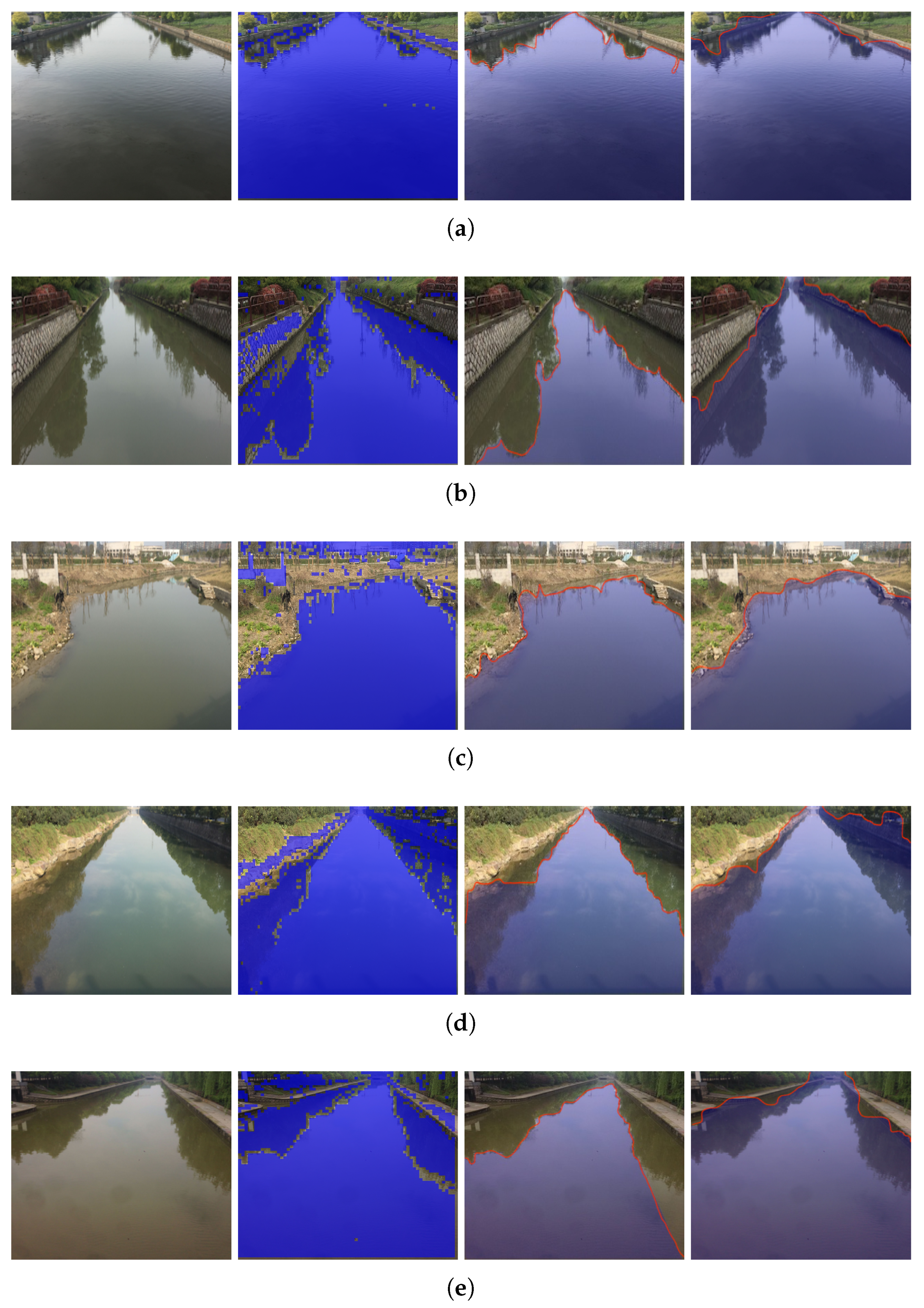
3.2. Experiments in Simple Scenes

The performance of different methods was evaluated by Pixel Accuracy( P A ), Mean Intersection over Union( M I o U ) which are two types of widely used criteria in image segmentation [30], shown as follows:
P A = i = 0 k p i i i = 0 k j = 0 k p i j ,
M I o U = 1 k + 1 i = 0 k p i i j = 0 k p i j + j = 0 k p j i p i i ,
where P i j indicates the number of pixels of class i that are predicted to belong to class j, where there are k + 1 classes in total. In this study, k + 1 = 2 . To better evaluate the overall segmentation performance, P A and M I o U , which may have different weights in practical applications, were merged to generate the weighted harmonic mean F β as:
F β = 1 + β 2 P A × M I o U β 2 × P A + M I o U ,
where β > 0 measures the relative importance between P A and M I o U . When β > 1 , M I o U has a greater impact. In practice, M I o U was slightly more important, thus β = 1.5 is adopted.
The results of some examples are shown in Figure 10 where the detected water region by “intensity + texture” method is marked with blue, while those by “edge detection” and the proposed algorithm is highlighted in red for edges. Table 1. shows the criteria values of the result.
All the three algorithms achieved not bad segmentation results, which meant they were all effective for segmentation of simple river scenes. But the proposed algorithm had a more stable performance. More importantly, the proposed algorithm took the least time, as obviously shown in Figure 11.
The method utilizing “intensit + texture” features was not only to calculate the brightness and texture information of each small image patch, but also to achieve the decision by the result of the clustering algorithm. The edge detection-based method often obtained many edges at the initial time. The adaptive threshold method required a lot of calculations to pick the one that is most likely to be the edge of the river. Both of them required a large amount of computation. However, the algorithm designed in this paper was essentially a fast two-class classification process on each image patch by using a preset threshold. The improved LBP feature is based on the comparison of intensity of neighbor pixels instead of exact calculations. Therefore, the proposed algorithm consumed the least time.

3.3. Experiments in Complex Scenes

Besides the simple river scenes, there are also some complex outdoor scenes where the traditional algorithms are difficult to take effect or even fail. Tests of different methods on complex scenes were conducted, among which four typical examples are shown in Figure 12 with the corresponding criteria values shown in Table 2.
Moreover, Figure 13 shows the speed of different methods in complex river scenes.
The proposed algorithm showed robust performance in complex scenes, and it got the highest F β and the least time cost compared with other methods. The proposed algorithm is proved effective and has better segmentation performance of river images.
The method utilizing “intensity + texture” features was prone to false detection. As shown in Figure 12, some pixels on the riverside were also detected as water. This is because some parts of the riverside in the image had similar features to the designed one. Therefore, the method simply using global image features could be confused. As for the method based on edge detection, it was likely to miss part of the water region with shadow due to the strong edge of clear shadow. This method could not distinguish whether the detected edge was a riverbank or other edges, which resulted in mistakes. However, the improved LBP and H variance features designed in this study were local features based on the water surface reflection mechanism, which was close to characteristics of water pixels. Such features could describe not only common water part of the image, but also those with complex appearance like light and covered shadow. To illustrate this, the results of each step in our algorithm are shown in Figure 14 to show how it works.

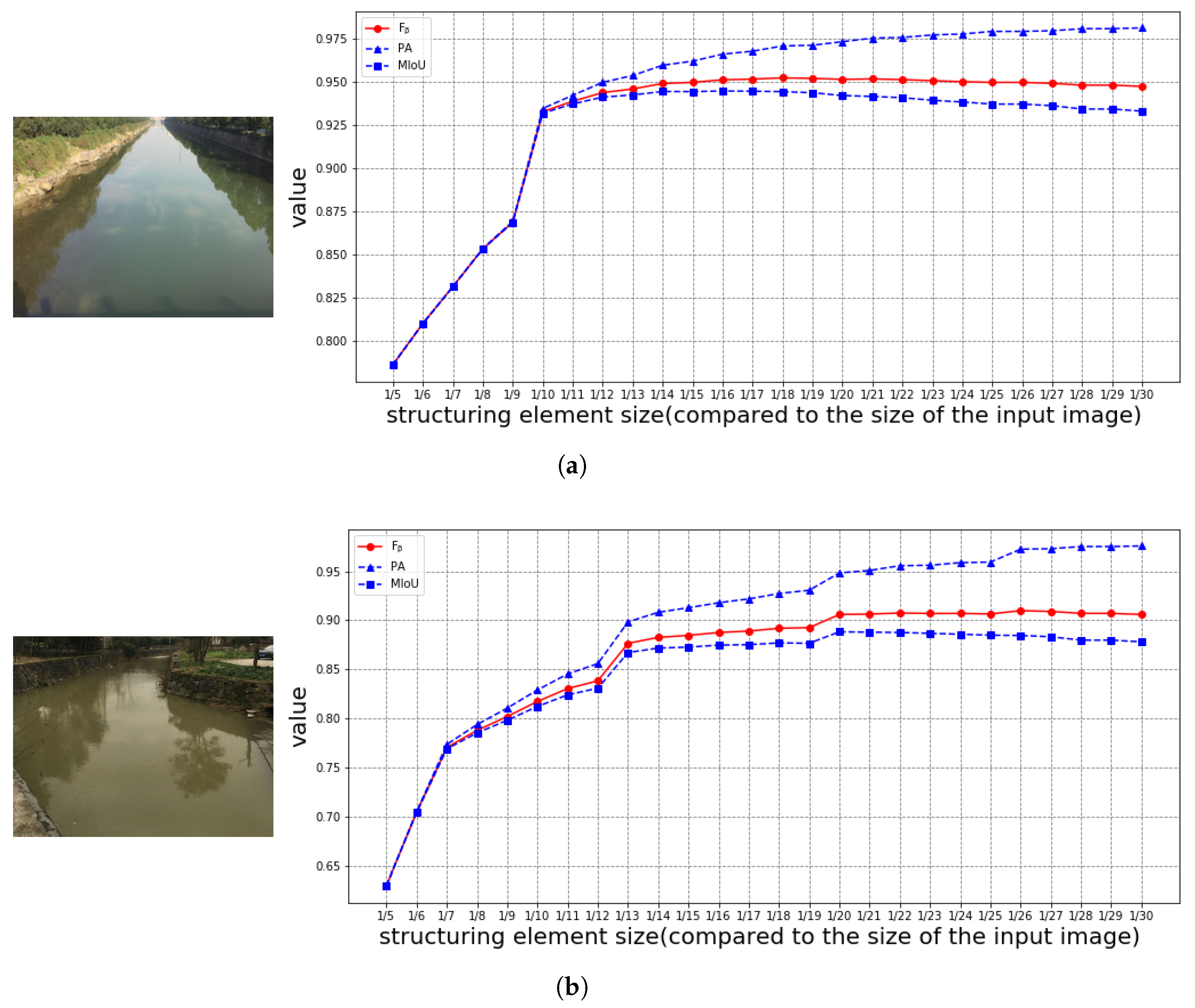
3.4. Discussion of Patch Size

The patch size, that is, the size of each detection window in the image, was the basic unit in the feature extraction operation in our algorithm. Theoretically, using a smaller patch size is faster in feature extraction, but the total times of feature calculation will increase, while the larger patch size made each patch contain more pixels, which might include negative samples (non-water pixels) that damaged the judgment of segmentation algorithm. Figure 15 shows the segmentation results using different patch sizes in our algorithm.
The F β and speed under different patch sizes were shown in Figure 16. With the patch size increased, F β ( β = 1.5 , see Equation (20)) reduced and the time cost was lower. After comprehensive consideration of the segmentation performance and time consumed, a 6 × 6 patch size is usually adopted in practice.

3.5. Discussion of Structuring Element

The size and shape of the structuring elements affected the final segmentation result. Some tests were performed on different resolution images using different sizes of structuring elements from 1/5 to 1/30 of the input image size. Two examples with criteria measuring the segmentation performance were shown in Figure 17.
As shown in the results, when the size of the structuring element grew larger than 1/15 of the input image size, the segmentation performance distinguishes little. Based on more experiments on the dataset, the size could be set to 1/15 of the size of the input image, where the algorithm was usually effective and reliable.

4. Conclusions

In this study, we focus on the image segmentation of outdoor river scenes. To solve the problem that current methods often missed detection and made false segmentations when applied to complex river scenes, this study proposed a novel segmentation method based on a reflection mechanism of the water surface. An improved LBP feature descriptor was designed for water detection and H variance was introduced to detect the shadow area of the water’s surface. Morphological operation with multiple dilation was employed to eliminate pseudo-water patches wrongly detected by the proposed algorithm and to obtain the largest connected domain in the image as water region. The experiments were performed in simple and complex river scenes respectively where the proposed method was compared with two other river segmentation methods. The results showed the proposed method took the least time and had better and robust performance in both simple and complex river scenes.
At present, the proposed algorithm has only been proven to be suitable for segmenting water parts in river images. Since the algorithm is designed based on the reflection mechanism of the water surface, it remains to be further studied whether it is effective for other types of images. The design ideas of the proposed algorithm may be helpful to other segmentation algorithms.
In the future, research can be conducted on anomaly detection of water surfaces based on the proposed method. This study is also important for unmanned surface vehicles (USVs) and river mapping.

Author Contributions

Conceptualization, J.Y.; Methodology, Y.L.; Data curation, Y.Z.; Supervision, P.H., J.Y., G.Z. and D.H.; Validation, W.X.; Writing—original draft, Y.L.; Writing—review & editing, P.H., J.Y. and D.H. All authors have read and agreed to the published version of the manuscript.

Funding

This work was funded by the Fundamental Research Funds for the Central Universities (No.2019QNA5015), the National Natural Science Foundation of China (No. 61803333, 61573313), the Key Technology Research and Development Program of Zhejiang Province (No.2015C03G2010034), and the National Key R&D Program of China (No.2017YFC1403801).

Conflicts of Interest

The authors declare no conflict of interest.

References

  1. Matthies, L.H.; Bellutta, P.; McHenry, M. Detecting water hazards for autonomous off-road navigation. In Proceedings of the Unmanned Ground Vehicle Technology V, Orlando, FL, USA, 21–25 April 2003; Volume 5083, pp. 231–242. [Google Scholar]
  2. Yu, J.J.; Luo, W.T.; Xu, F.H.; Wei, C.Y. River boundary recognition algorithm for intelligent float-garbage ship. Electron. Des. Eng. 2018, 2018, 29. [Google Scholar]
  3. Song, Y.; Wu, Y.; Dai, Y. A new active contour remote sensing river image segmentation algorithm inspired from the cross entropy. Digit. Signal Process. 2016, 48, 322–332. [Google Scholar] [CrossRef]
  4. Ciecholewski, M. River channel segmentation in polarimetric SAR images: Watershed transform combined with average contrast maximisation. Expert Syst. Appl. 2017, 82, 196–215. [Google Scholar] [CrossRef]
  5. Han, B.; Wu, Y. A novel active contour model based on modified symmetric cross entropy for remote sensing river image segmentation. Pattern Recognit. 2017, 67, 396–409. [Google Scholar] [CrossRef]
  6. Lopez-Fuentes, L.; Rossi, C.; Skinnemoen, H. River segmentation for flood monitoring. In Proceedings of the 2017 IEEE International Conference on Big Data (Big Data), Boston, MA, USA, 11–14 December 2017; pp. 3746–3749. [Google Scholar]
  7. Rankin, A.L.; Matthies, L.H.; Huertas, A. Daytime water detection by fusing multiple cues for autonomous off-road navigation. In Transformational Science And Technology For The Current And Future Force: (With CD-ROM); World Scientific: Singapore, 2006; pp. 177–184. [Google Scholar]
  8. Yao, T.; Xiang, Z.; Liu, J.; Xu, D. Multi-feature fusion based outdoor water hazards detection. In Proceedings of the 2007 International Conference on Mechatronics and Automation, Harbin, China, 5–8 August 2007; pp. 652–656. [Google Scholar]
  9. Zhao, J.; Yu, H.; Gu, X.; Wang, S. The edge detection of river model based on self-adaptive Canny Algorithm and connected domain segmentation. In Proceedings of the 2010 8th World Congress on Intelligent Control and Automation, Jinan, China, 7–9 July 2010; pp. 1333–1336. [Google Scholar]
  10. Wei, Y.; Zhang, Y. Effective waterline detection of unmanned surface vehicles based on optical images. Sensors 2016, 16, 1590. [Google Scholar] [CrossRef] [PubMed] [Green Version]
  11. Sun, Y.; Fu, L. Coarse-fine-stitched: A robust maritime horizon line detection method for unmanned surface vehicle applications. Sensors 2018, 18, 2825. [Google Scholar] [CrossRef] [Green Version]
  12. Achar, S.; Sankaran, B.; Nuske, S.; Scherer, S.; Singh, S. Self-supervised segmentation of river scenes. In Proceedings of the 2011 IEEE International Conference on Robotics and Automation, Shanghai, China, 9–13 May 2011; pp. 6227–6232. [Google Scholar]
  13. Zhan, W.; Xiao, C.; Wen, Y.; Zhou, C.; Yuan, H.; Xiu, S.; Zhang, Y.; Zou, X.; Liu, X.; Li, Q. Autonomous Visual Perception for Unmanned Surface Vehicle Navigation in an Unknown Environment. Sensors 2019, 19, 2216. [Google Scholar] [CrossRef] [Green Version]
  14. Han, X.; Nguyen, C.; You, S.; Lu, J. Single Image Water Hazard Detection using FCN with Reflection Attention Units. In Proceedings of the European Conference on Computer Vision (ECCV), Munich, Germany, 8–14 September 2018; pp. 105–120. [Google Scholar]
  15. Hong, T.H.; Rasmussen, C.; Chang, T.; Shneier, M. Fusing ladar and color image information for mobile robot feature detection and tracking. In Proceedings of the 7th International Conference on Intelligent Autonomous Systems, Marina del Rey, CA, USA, 25–27 March 2002; Gini, M., Shen, W.-M., Torras, C., Yuasa, H., Eds.; IOS Press: Amsterdam, The Netherlands, 2002; pp. 124–133. [Google Scholar]
  16. Nguyen, C.V.; Milford, M.; Mahony, R. 3D tracking of water hazards with polarized stereo cameras. In Proceedings of the 2017 IEEE International Conference on Robotics and Automation (ICRA), Singapore, 29 May–3 June 2017; pp. 5251–5257. [Google Scholar]
  17. Kim, J.; Baek, J.; Choi, H.; Kim, E. Wet area and puddle detection for Advanced Driver Assistance Systems (ADAS) using a stereo camera. Int. J. Control Autom. Syst. 2016, 14, 263–271. [Google Scholar] [CrossRef]
  18. Pandian, A. Robot Navigation Using Stereo Vision and Polarization Imaging. Master’s Thesis, Institut Universitaire de Technologie IUT Le Creusot, Universite de Bourgogne, Le Creusot, France, 2008. [Google Scholar]
  19. Yang, K.; Wang, K.; Cheng, R.; Hu, W.; Huang, X.; Bai, J. Detecting traversable area and water hazards for the visually impaired with a pRGB-D sensor. Sensors 2017, 17, 1890. [Google Scholar] [CrossRef] [PubMed] [Green Version]
  20. Iqbal, M.; Morel, M.; Meriaudeau, F. A survey on outdoor water hazard detection. In Skripsi Program Studi Siste Informasi; University of Southampton: Southampton, UK, 2009. [Google Scholar]
  21. Rankin, A.; Matthies, L. Daytime water detection based on color variation. In Proceedings of the 2010 IEEE/RSJ International Conference on Intelligent Robots and Systems, Taipei, Taiwan, 18–22 October 2010; pp. 215–221. [Google Scholar]
  22. KOEN, E. Evaluation of color descriptors for object and scene recognition. In Proceedings of the IEEE Conference on Computer Vision and Pattern Recognition, Anchorage, AK, USA, 23–28 June 2008. [Google Scholar]
  23. Xu, M.; Ellis, T. Illumination-Invariant Motion Detection Using Colour Mixture Models. In BMVC; Citeseer: Princeton, NJ, USA, 2001; pp. 1–10. [Google Scholar]
  24. Gonzalez, R.C.; Wintz, P. Digital Image Processing; Number 13; Addison-Wesley Pub. Co.: Boston, MA, USA, 1977; p. 451. [Google Scholar]
  25. Haralick, R.M.; Shanmugam, K. Textural features for image classification. IEEE Trans. Syst. Man Cybern. 1973, 3, 610–621. [Google Scholar] [CrossRef] [Green Version]
  26. Laws, K.I. Rapid texture identification. In Proceedings of the Image Processing for Missile Guidance, San Diego, CA, USA, 29 July–1 August 1980; Volume 238, pp. 376–381. [Google Scholar]
  27. Guo, Z.; Zhang, L.; Zhang, D. A completed modeling of local binary pattern operator for texture classification. IEEE Trans. Image Process. 2010, 19, 1657–1663. [Google Scholar] [PubMed] [Green Version]
  28. Serra, J. Image Analysis and Mathematical Morphology; Academic Press, Inc.: Cambridge, MA, USA, 1983. [Google Scholar]
  29. Haralick, R.M.; Sternberg, S.R.; Zhuang, X. Image analysis using mathematical morphology. IEEE Trans. Pattern Anal. Mach. Intell. 1987, 9, 532–550. [Google Scholar] [CrossRef] [PubMed]
  30. Garcia-Garcia, A.; Orts-Escolano, S.; Oprea, S.; Villena-Martinez, V.; Martinez-Gonzalez, P.; Garcia-Rodriguez, J. A survey on deep learning techniques for image and video semantic segmentation. Appl. Soft Comput. 2018, 70, 41–65. [Google Scholar] [CrossRef]
Figure 1. Flowchart of the proposed algorithm.
Applsci 10 02471 g001
Figure 2. Light path diagram of river scene.
Applsci 10 02471 g002
Figure 3. Relationship between water surface reflection and horizontal distance l with different heights camera.
Applsci 10 02471 g003
Figure 4. Pixel-wise intensity values and hue values in a column of river scene image.
Applsci 10 02471 g004
Figure 5. Illustration of generation of image patches.
Applsci 10 02471 g005
Figure 6. Color space conversion and image division for local hue variance calculation.
Applsci 10 02471 g006
Figure 7. Morphological operation method designed in our algorithm.
Applsci 10 02471 g007
Figure 8. Pre-processing operations.
Applsci 10 02471 g008
Figure 9. Pixel values before and after blurring operation.
Applsci 10 02471 g009
Figure 10. Segmentation results of different methods in simple scenes (ae). From left to right, the first column shows the input images after pre-processing; The second and third column are the segmentation results using “intensity + texture” features and the adaptive threshold edge detection algorithm respectively; The fourth column are the results of our method.
Applsci 10 02471 g010
Figure 11. Speed of different methods in simple scenes.
Applsci 10 02471 g011
Figure 12. Segmentation results of different algorithms in complex scenes (ad). From left to right: The first column are the input images after pre-processing; The second and third column are respectively the segmentation results using “intensity + texture” features and the adaptive threshold edge detection algorithm; The fourth column are the results of our method.
Applsci 10 02471 g012
Figure 13. Speed of different methods in the complex scenes.
Applsci 10 02471 g013
Figure 14. Performance of the proposed method in complex scenes (ad). From left to right, the first column includes the images after pre-processing. In the second column, The blue squares in images represent the detection result of water region with the improved LBP feature. In the third column the green squares represent the detection result by H-variance feature developed from the second column images. The fourth column images are the binary mask of detection results after the designed morphological operation. The fifth column images are final segmentation results of river region indicated by a covered translucent blue area.
Applsci 10 02471 g014aApplsci 10 02471 g014b
Figure 15. Segmentation results under different patch sizes from 6 × 6 to 36 × 36 pixels used in the proposed algorithm.
Applsci 10 02471 g015
Figure 16. Performance of the proposed algorithm under using different patch sizes. (a) P A , M I o U and F β under different patch sizes. (b) Speed under different patch sizes.
Applsci 10 02471 g016
Figure 17. Performance under different sizes of structuring elements in the proposed algorithm. (a) An example of simple river scene; (b) An example of complex river scene.
Applsci 10 02471 g017
Table 1. Performance of different methods in simple scenes.
River SceneIntensity + TextureEdge DetectionOur Algorithm
PAMIoU F β PAMIoU F β PAMIoU F β
(a)0.9970.9150.9390.9640.9260.9370.9870.9690.967
(b)0.9010.8240.8460.9950.5920.6760.9530.9280.948
(c)0.8370.8210.8260.9760.9320.9450.9810.9470.956
(d)0.9200.8510.8710.9930.8290.8730.9740.9270.946
(e)0.9210.8810.8930.9980.7460.8090.8710.9570.969
Average of 110 images0.9150.8470.8670.9730.7950.8420.9660.9230.938
Table 2. Performance of different methods in complex scenes.
River SceneIntensity + TextureEdge DetectionOur Algorithm
PAMIoU F β PAMIoU F β PAMIoU F β
(a)0.9080.7080.7590.9870.6290.7080.9080.8780.887
(b)0.8640.8220.8340.9990.7220.7890.9480.9100.921
(c)0.6570.6640.6620.9950.8450.8860.9130.8730.885
(d)0.8540.7750.7980.9810.8300.8710.9340.9310.932
Average of 390 images0.8020.7450.7620.9850.7450.8050.9350.9250.929

