1. Introduction
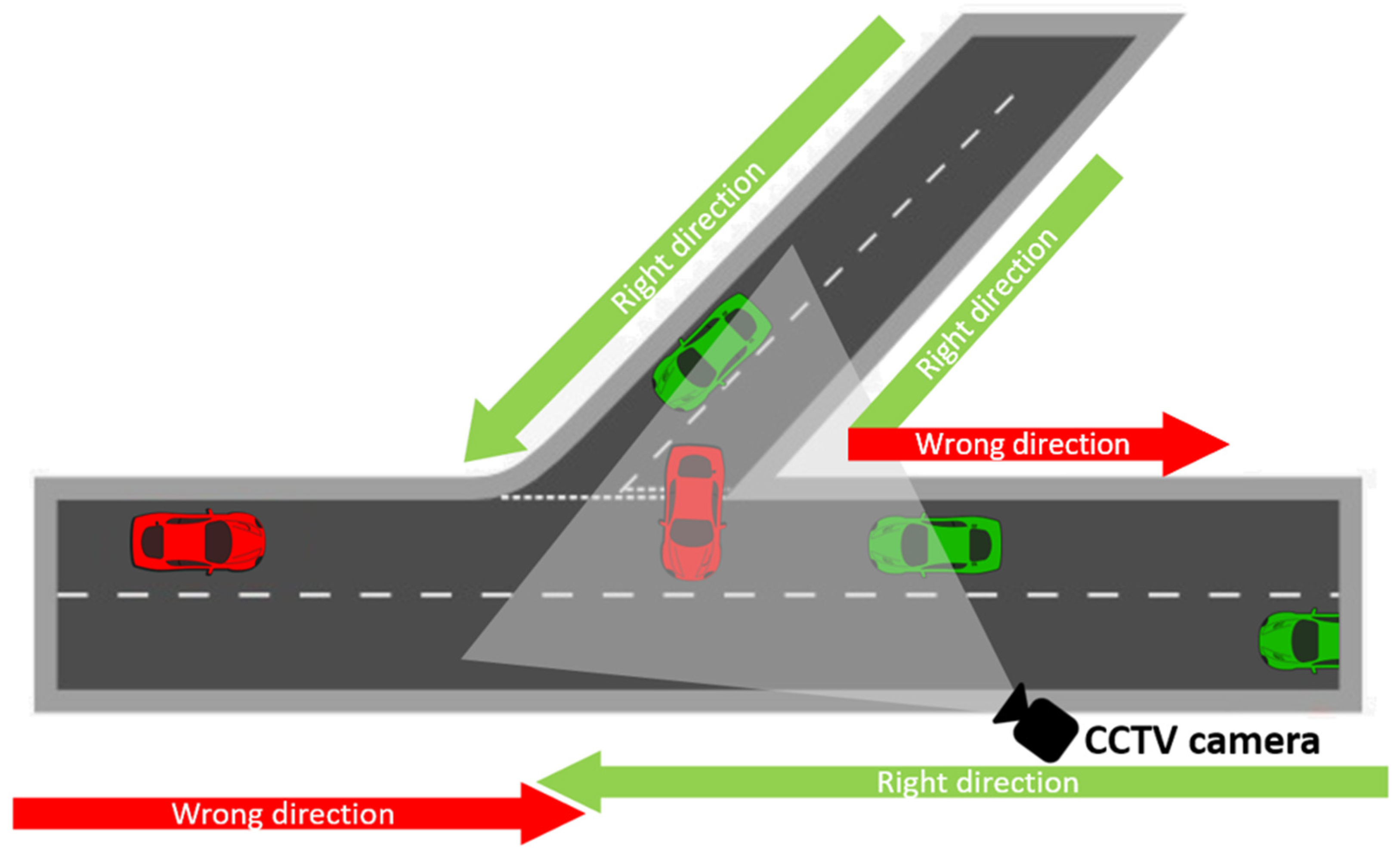
With the development of the fourth industrial revolution, the role of the intelligent transportation system (ITS) is becoming more and more crucial for ensuring the safety and efficiency of drivers. The purpose of a vision-based ITS is to extract useful and precise traffic data, and to use surveillance technologies as efficiently as possible. According to the National Information Society Agency, there were more than eight million closed-circuit television (CCTV) cameras installed in Korea by the year 2018, which gives the country one of the highest cameras-per-capita rates in the world. CCTV footage certainly cannot be a perfect solution for all traffic violations. However, it is widely and increasingly used by government officials to identify serious violations, along with evidence, testimonies, and documents. Typically, driving the wrong way down a road happens for several reasons: the driver is distracted or confused; the driver did not notice the pavement markings or traffic signs; the driver intentionally breaks the rules; etc. Even though recent pavement delineations and signs are innovative, they might not be enough to alert drivers to wrong-way entry, and car accidents continue to happen. Even though it is almost impossible to control human driving behavior, it is important to classify and understand irregular activity in usual traffic scenarios in order to prevent serious car crashes. So far, the identification task is performed by people who work in monitoring companies. Nevertheless, with the significant increase in camera devices, the need for automated intelligent software is demanded even more. Wrong-direction detection technologies can be divided into three major categories: sensor-based detection, radar-based detection, and video imaging-based detection. The focus of this research is to automate the recognition of moving violations, thus requiring less human interaction, as well as to identify (using a single video camera) vehicles entering traffic the wrong way onto the highway system (
Figure 1).
While our proposed system relies on video imaging-based detection, it references three different computer vision challenges such as vehicle’s localization, tracking, and determining direction. Vision-based learning is one of the cheapest methods and requires lower labor costs by saving people’s time, as well as lowering costs by using fewer machines and by eliminating faulty products.
2. Background
To determine a car’s direction, the car itself should be identified, so detection is the first step in our research. Wrong direction estimation is not a contemporary problem, and in this section, we describe and implement different techniques in computer vision to compare different detection and tracking algorithms for vehicles. These techniques include well-known machine learning and deep learning methods.
2.1. Vehicle Detection and Segmentation
2.1.1. Detection Using Background Subtraction
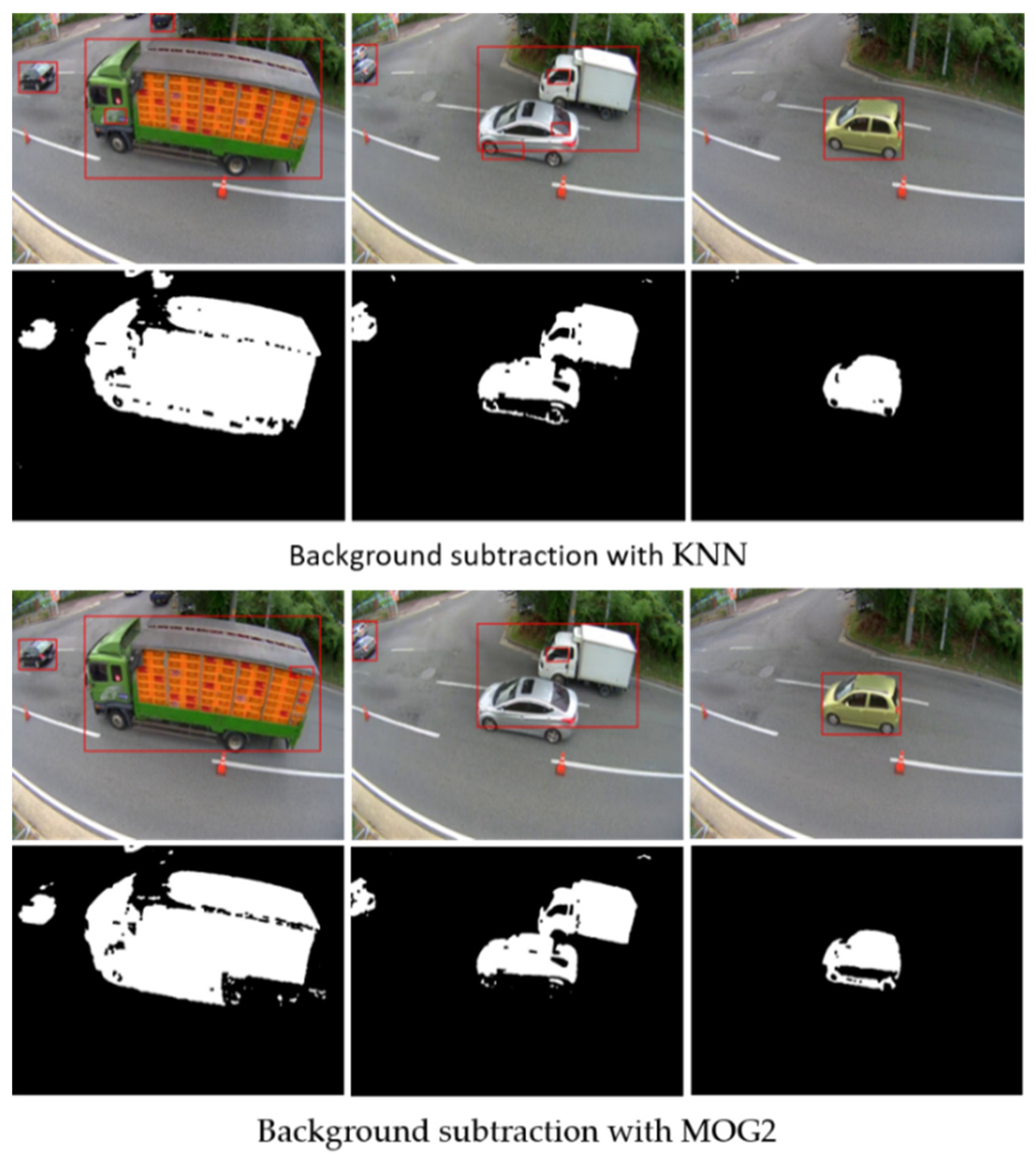
Background subtraction (BS) is a widely used technique for applying a foreground mask for static cameras. Moving objects in the foreground are separated by calculating the foreground mask and subtracting it from the current frame and background model, containing the static part of the scene. Everything moving is considered characteristic of the foreground. BS is performed using two main functions: background initialization and background update. BS algorithms have already been implemented in open-source computer vision libraries such as OpenCV. In OpenCV, two background subtraction methods were implemented: k-nearest neighbor (KNN) algorithm [
1] and Gaussian mixture-based background/foreground segmentation algorithm (MOG2) [
2,
3].
BS showed instability on the false positive detections when it detected several closely located cars as one (
Figure 2). The method is very sensitive to changing lighting conditions and, as an example, the results obtained during nighttime could be unacceptably inaccurate.
2.1.2. Optical Flow
One of the machine learning methods for locating a car is an optical flow which is the pattern learning of a moving object. The most widely used optical flow method in computer vision is called the Lucas–Kanade method [
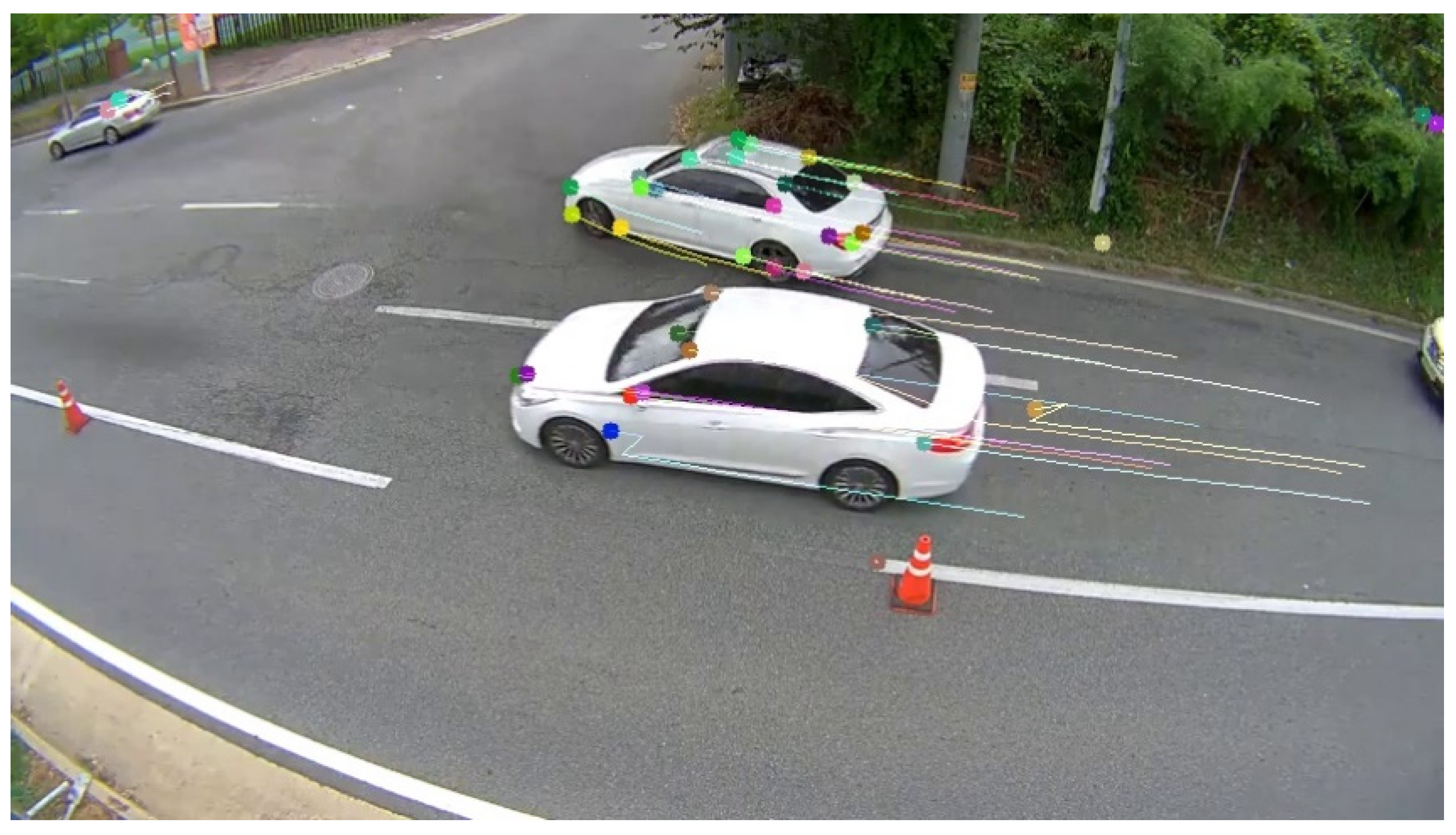
4]. The basic idea of optical flow is to assume that the color or intensity of a pixel is constant under displacement from one frame to the next. This optical flow estimation algorithm also assumes that an object’s frame-to-frame displacement distance is small and local. In addition, the objective measurement of the local level of reliability of motion information is provided. Shi and Tomasi [
5] increased tracking performance by modifying the “good feature” selection criterion of reliability in order to evaluate the texture features of areas, which later led to the creation of the Kanade–Lucas–Tomasi (KLT) tracker [
6] (see
Figure 3). However, according to Barron et al. [
7], optical flow computation techniques are very sensitive to noise and object illumination. Generally, optical flow can be unreliable in cases where the brightness intensity changes, and object occlusions happen. Since our task in focus requires a minimal error rate, usage of optical flow as a detector could be unacceptable due to the changing lighting and weather conditions.
Monteiro et al. [
8] described optical flow-based wrong-way driver detection. Their proposed system was separated into three main stages: learning, detection, and validation. For the learning stage, which is the car detection phase, they combined the Lucas–Kanade optical flow method with Gaussian mixture models [
9]. They mentioned that their system could detect vehicles moving in the wrong direction from a 320 × 240 pixel image at 33 frames per second (fps). Accordingly, the experiments conducted on many scenes demonstrated that their proposed system has the following properties: wrong-way vehicle detection, speed, and robustness to illumination and weather conditions. However, the simulation results and experiments on system accuracy were insufficient to prove the applicability of their method.
2.1.3. Convolutional Neural Network (CNN)-Based Detection Methods
Convolutional neural networks (CNNs) are predominantly used as learning structures for image understanding. The benefits of using CNNs are that fewer learning parameters might be used, which greatly improves the learning time and reduces the amount of data required to train the model. A convolution is a weighted sum of the pixel values of an image as the window slides across the whole image. Basically, the convolution process throughout an image with a weight matrix produces another image. The CNN-based approach may be considered one of the best ways to precisely detect a vehicle’s position in an image, and so far, it includes sophisticated methods such as the single shot multiBox detector (SSD) [
10], the faster regional CNN (faster R-CNN) [
11], and you only look once (YOLO) [
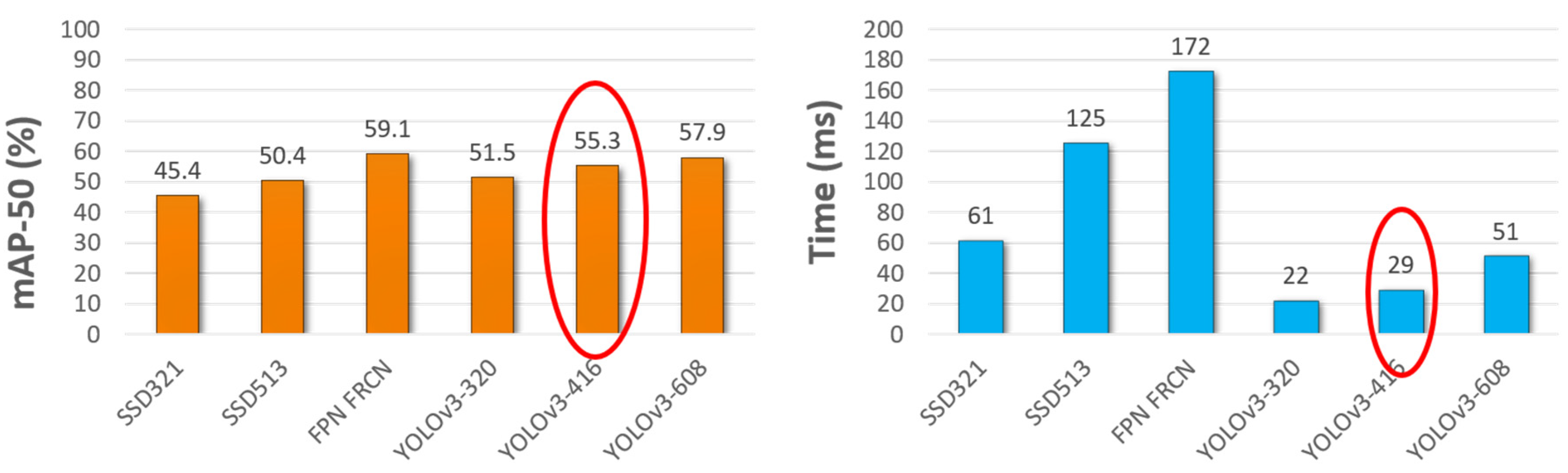
12]. All these methods have a similar average precision on detections. However, there is a significant difference in the inference time with each method. Although the faster R-CNN (a region proposal network) was the best detection method on Pascal Visual Object Classes (VOC) and Common Objects in Context (COCO) dataset challenges in 2012 and 2015, respectively, we decided to use the YOLOv3 network due to the speed performance.
As
Figure 4 shows, all the compared methods have similar mean average precision, but with a huge gap between them for processing times. Since our project is highly reliant on fast processing, we chose to use YOLOv3-416 which took 29 ms to process the COCO dataset.
2.2. Vehicle Tracking
Car tracking is based on object-tracking techniques and includes three main processes: (1) taking an initial set of detected objects; (2) registering the detected cars and giving them unique identifications (IDs); (3) tracking them as they move around a continuous frame, maintaining the ID assignments, and erasing them once the cars disappear. Moreover, object tracking allows us to count several cars in a frame by counting unique object IDs. Ideally, an object tracking algorithm must satisfy the following conditions:
require the object detection phase only once;
be much faster than the actual object detector itself;
handle a tracked object that “disappears”;
be robust to occlusions;
pick up objects that are “lost” between frames.
2.2.1. Contour-Based Tracking
The main idea behind contour-based tracking is to define the boundaries of a vehicle. Ambardekar et al. [
14] proposed pose detection of a vehicle by using optical flow and camera parameters. According to the authors, part of the system tracks the blobs and tries to correct the errors from the foreground object detection module by estimating the three-dimensional (3D) world coordinates of the points on the vehicles. The system then groups those points together to segment and track the individual vehicles. The authors emphasized that their proposed technique has occlusion detection and multi-vehicle tracking [
15].
2.2.2. Kalman Filter for Tracking
Kalman filtering also known as linear quadratic estimation (LQE) is a series of measurements observed over time (in our case, frame by frame). The Kalman filter is a powerful tracking method, for extracting motion from video sequence surfaces over collections of points. It is an optimal estimator that infers the parameters of interest from indirect, inaccurate, and uncertain observations. The Kalman filter consists of two steps: prediction and update. The first step uses previous states to predict the current state. The second step uses the current measurement, such as detection of bounding box location, to correct the state. The Kalman filter has the following important features that tracking can benefit from:
predict the object’s upcoming location;
correct the prediction based on new measurements;
reduce noise introduced by inaccurate detection;
facilitate the process of associating multiple objects with their tracks.
The Kalman filter tracker is fast, which is an advantage over other tracking algorithms. Therefore, we updated the original algorithm and used it in our project as the main tracking method.
Despite quite the variety of methods, we focus on improving the time speed of detection, robustness in different lighting conditions, and accuracy. Therefore, we combined the YOLOv3 method for detection with the Kalman filter for tracking estimation.
3. Proposed System
3.1. Detection and Tracking
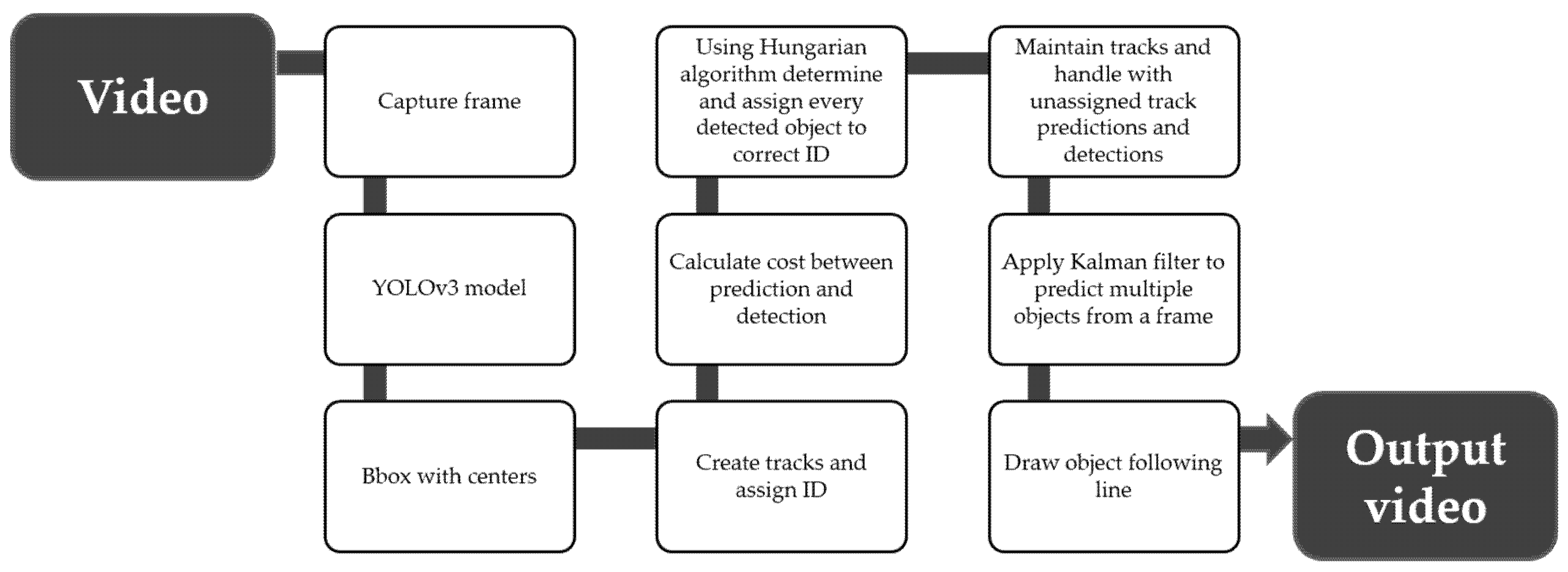
We separate our task into three main steps: detection, tracking, and direction checking. YOLOv3 is an object detection method targeted at real-time video processing. The result of the YOLOv3 model extracts a vehicle’s bounding box information in order to apply robust tracking algorithms and identify direction.
First, we send a continuous frame to the pre-trained YOLOv3 model that returns us bounding boxes of vehicles. Our algorithm is based on centroid tracking, which is a multi-step process. Centroid tracking assumes that we are passing (
x,
y)-coordinates in a set of bounding boxes for each detected object in each frame. Once we have the bounding box coordinates, we compute the “centroid” (i.e., the center (
x,
y)) coordinates of the bounding boxes. Since these are the initial set of bounding boxes presented to our algorithm, we assign them unique IDs. Then, we calculate the cost value between the detected car and its prediction. If there are multiple detections, we need to assign each of them to a tracker. We use intersection over union (IOU) of the tracker bounding box and detection bounding box as a metric. We maximize the sum of the IOU assignment using the Hungarian algorithm [
16]. The machine learning package scikit-learn has a build-in utility function that implements the Hungarian algorithm. Then we implement updated Kalman filter equations that are described by Welch and Bishop [
17] to predict multiple car objects from a video frame.
Prediction phase
Notations:
x—state mean,
P—state covariance,
F—state transition matrix,
Q—process covariance,
B—control function (matrix),
u—control input.
Update phase
Notations:
H—measurement function (matrix),
z—measurement,
R—noise covariance,
y—residual,
K—Kalman gain.
The formula for the updated (a posteriori) state estimate works each time for the measurement update pair. The process is repeated with the previous (a posteriori) estimates used to project or predict the new (a priori) estimates. An implementation of the updated Kalman filter algorithm can be found in
Algorithm 1. Then we used OpenCV drawing libraries to draw tracking lines on each detected car.
Figure 5 presents the full pipeline of our proposed method.
| Algorithm 1. Pseudo-code for Kalman filter tracker. |
Object tracking function (x, y centroid)
for (iterate ≥ number of detected centroids):
if (no track vectors found)
Create tracks
Calculate cost using sum of square distance
Assign detected measurements to predicted classes using Hungarian algorithm
if (tracks with no assignment)
Identify tracks
if (tracks are not detected for long time)
Delete tracks
else
Start new tracks
Update Kalman Filter state, last results and tracks trace |
3.2. Direction Estimation
This section describes the method for vehicle trajectory estimation. To check the direction of a tracked vehicle we calculate the difference in the pixels in the F
N-frames range, where
N- is the number of frames to track a unique vehicle. First, we calculate the centroid from a detected car’s bounding box and set it to be the initial points (
X0,
Y0) in the frame (
F0). Then, as the car moves, the position of the centroid changes from frame to frame. Thus, we calculate the pixel difference in the range (
X1,
Y1) to (
XN,
YN) for each frame, where
X1,
Y1 indicates the car’s centroid position in the frame (
F1), along with
XN and
YN in frame (
FN). For example, let us assume we use six frames for tracking. The pixel position difference would be
X5 −
X1. Basically, we take the second frame as an initial starting point and the sixth frame as the ending point. This is due to the ID assignment step that is done on the first frame as soon as a car is detected. To find the direction, we do simple math: if
is negative and
X5 is smaller than
X1, the car is moving from right to left; vice versa, then it is moving left to right.
Algorithm 2 describes the pseudo-code to validate the car’s direction.
| Algorithm 2. Pseudo-code for the direction check. |
if (length of centroids > 0)
for (iterate ≥ number of detected centroids):
for (iterate ≥ N, where N number of tracking frames for unique cars)
take X1, Y1 positions from tracker
take ID for unique car
= XN − X1 if (check sign and X1 with X2)
assign direction |
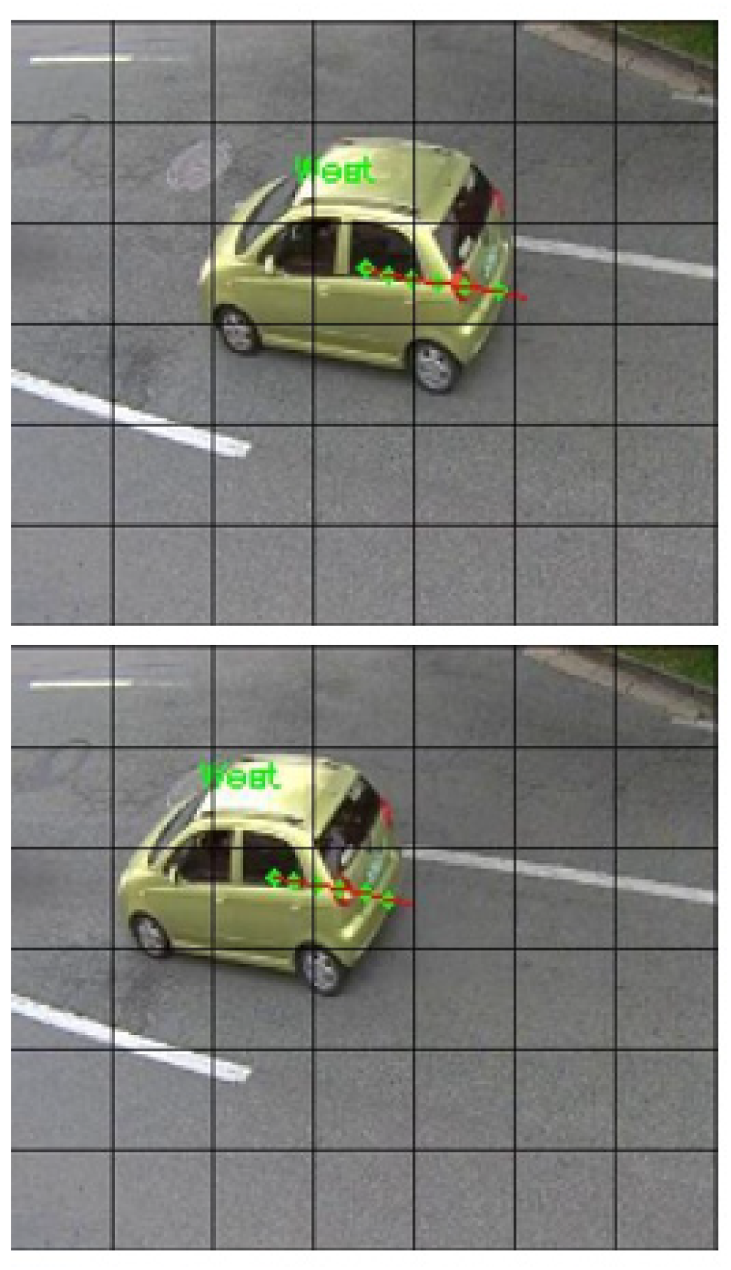
Figure 6 visually explains the changing vehicle’s position within
N = 6 frames. Green dots show the displacement of the car through each frame. The displayed text “West” in this case shows that the car in the video is moving from right to left.
3.3. Direction Validation
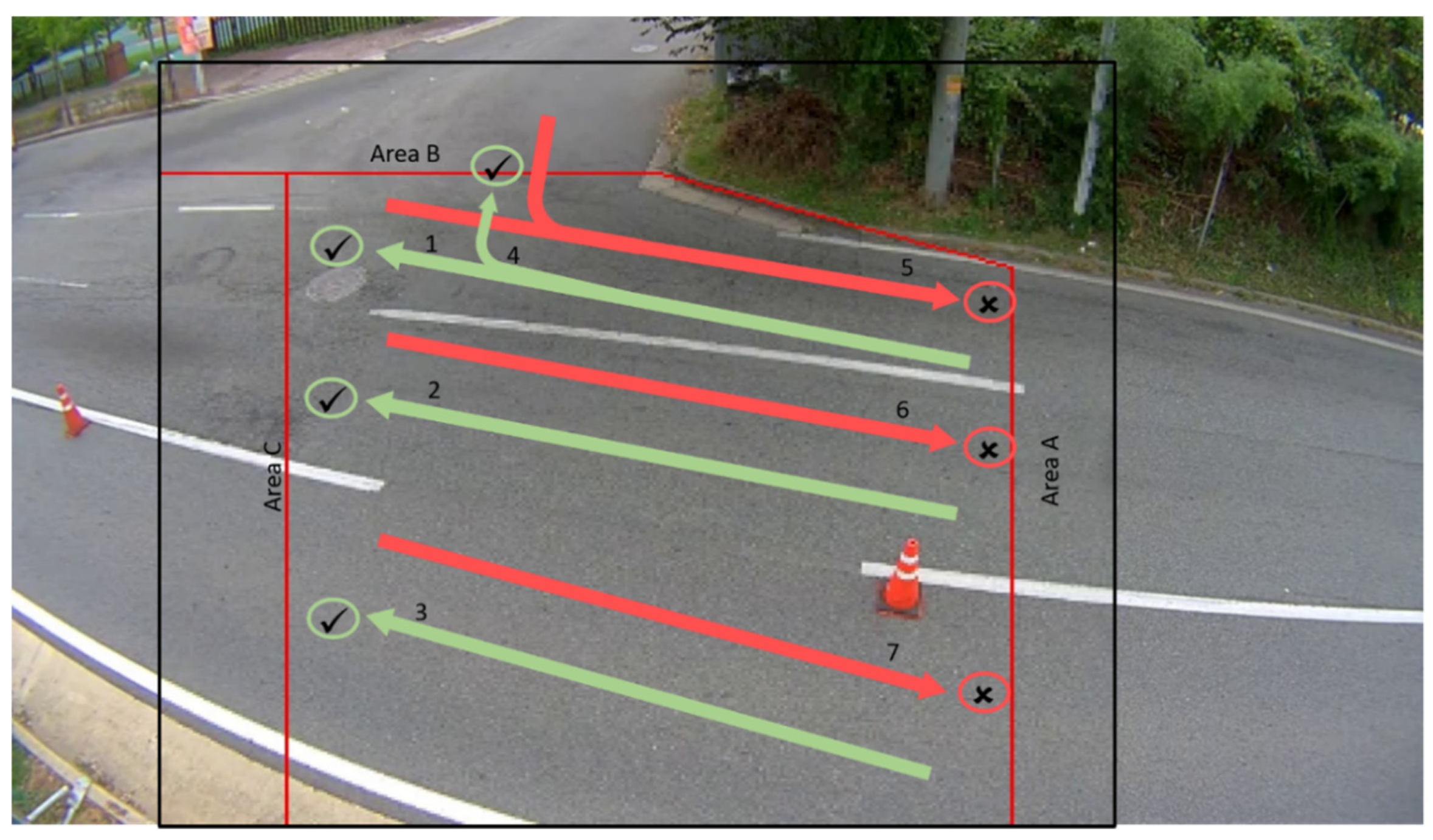
To determine if the car is going the right way, we created the entry-exit approach. The idea behind it is simple and effective. We create imaginary entry lines on the video frame. If a vehicle crosses the entry lines, the given unique ID of the car is stored in a list, and if it passes through the exit area the ID is removed from the list.
As seen in
Figure 7, we crop the video frame to the required region of interest. Traffic must go from the right side to the left (lines 1–4). Green lines represent correct entry and exit directions. Red lines represent directions in which vehicles must not move (lines 5–7). We create three imaginary areas for entering and exiting. Imagine the usual case when the car enters the first area. In such a case, when the car’s centroid passes through area A, the ID of the car is stored in list 1 and remains there until the car exists from any exit. If the car enters from area B, the ID is stored in list 2 and the car must exit in area C; otherwise, the car will be detected as the moving the wrong way, and a warning signal will be triggered. If the car enters in area C, this is always the wrong way and the ID of the car is stored in list 3 to check the area from which it exited. Even if a car enters from area C, the alert signal is sent when the car is moving. The algorithm validates according to the vehicle’s centroid position.
4. Experiments and Results
We conducted two types of experiments to check the efficiency of our work. The first consisted of checking the car-detection accuracy under different lighting conditions, and the second consisted of wrong-way driver detection. We were provided access to a real-world camera and created a simulation with a car moving the wrong way.
4.1. Datasets
Data used in our project were taken from a fixed CCTV camera. We create two types of datasets: one is for network training and testing and the other is for wrong direction checking. For the first dataset, we have extracted 12 videos taken at different times of the day. We extract all the frames from every video and randomly split them into training and testing at 70% and 30%, respectively. The second type of dataset is used to check the wrong-direction detection, so it contained only data of a car moving in the wrong way.
4.2. YOLOv3 Model Training
For the detection experiments, we trained the model by annotating real-world data. We had video files from which we extracted frames and created our own CCTV dataset. We annotated extracted images with a specific program [
18] and trained our YOLOv3 network using 1750 images on a PC with an NVidia RTX 2080Ti GPU, an Intel Core i5-7600 CPU, and 16 GB RAM. We chose YOLOv3-416, in which images are resized to 416 × 416 pixels, with learning rate α = 10
-3 batch size = 64 on frozen layers, and batch size = 8 for unfrozen ones, over 100 epochs. We used the Adam optimizer with α = 10
-3 for frozen layers and α = 10
-4 after unfreezing the layers. The YOLOv3 network convergence time depends on the quantity of data used in training; so, in our case, it took four to five hours to converge. Since our model is trained with images from the camera used in one fixed position our model applies only to the particular camera.
4.3. Detection Testing
To test detection performance, we created another dataset from unseen videos. Next, we manually calculated the number of cars appearing in those videos. Then, we randomly selected videos taken at different time intervals. We chose various time intervals including morning, afternoon, dusk, and evening times. For evaluating detection precision, we decided to calculate the mean average precision (mAP or μ) with IOU threshold
where the mAP with threshold is found by,
We manually counted the number of cars that appeared within the mentioned intervals and annotated them to determine the cars’ positions in a frame. We counted only unique cars. The car was considered as correctly detected one only when the IOU rate was above 0.75. As seen in
Table 1, the detection method identified cars with average mAP of 90.80% for both daytime and nighttime. The reason for the slight change in mAP is the different lighting conditions. Since our application is supposed to be used in real-world scenarios, we tested it for precision and speed. Therefore, along with precision, we also checked the processing time of our algorithm, which was similar to that of Redmon and Farhadi [
16]. Despite having only one class to detect, we achieved a higher mAP score than the authors of the original YOLOv3 (see
Figure 4).
4.4. Wrong-Direction Detection Testing
To justify the efficiency of our work, we provided a qualitative experiment. Testing wrong-way detection is based more from the structure of the related facts than from the testing of the existing assumption. Therefore, we tested our implemented “entry-exit” algorithm for wrong-direction detection on two types of data: real data and simulated data. Due to the difficulty in getting actual wrong way driving events, we simulated them by intentionally driving a car the wrong way. For the first simulation case, we checked daytime wrong-direction detection. As illustrated in
Figure 7, a car going the wrong way enters from area C and is tracked until it reaches area A, which in this case is where it exits. As soon as it reaches area C, image and information about the car were sent to the monitoring center using the File Transfer Protocol (FTP) and Transmission Control Protocol (TCP). The program detects moving vehicles from an 807 × 646 video frame at 30 fps.
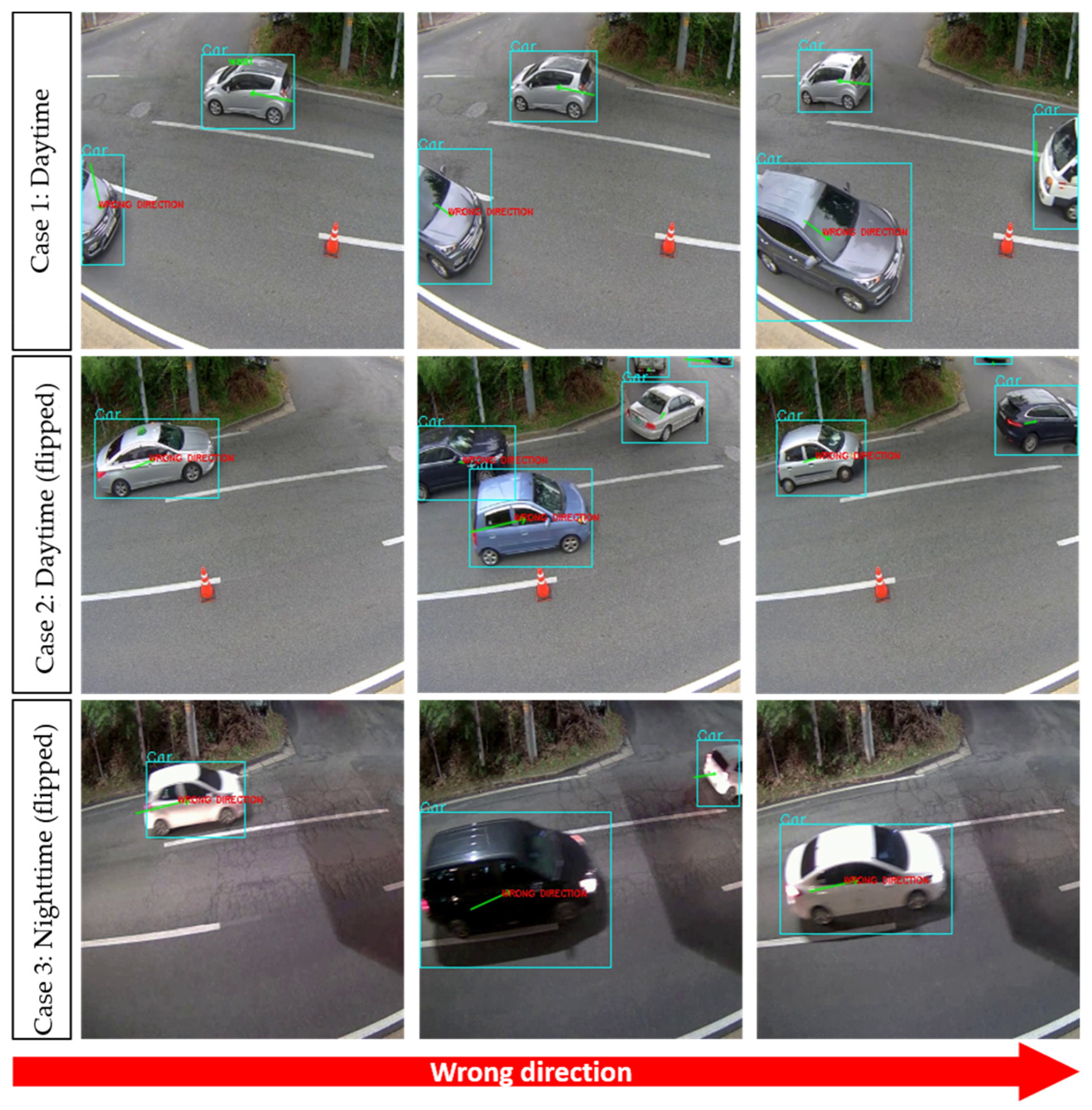
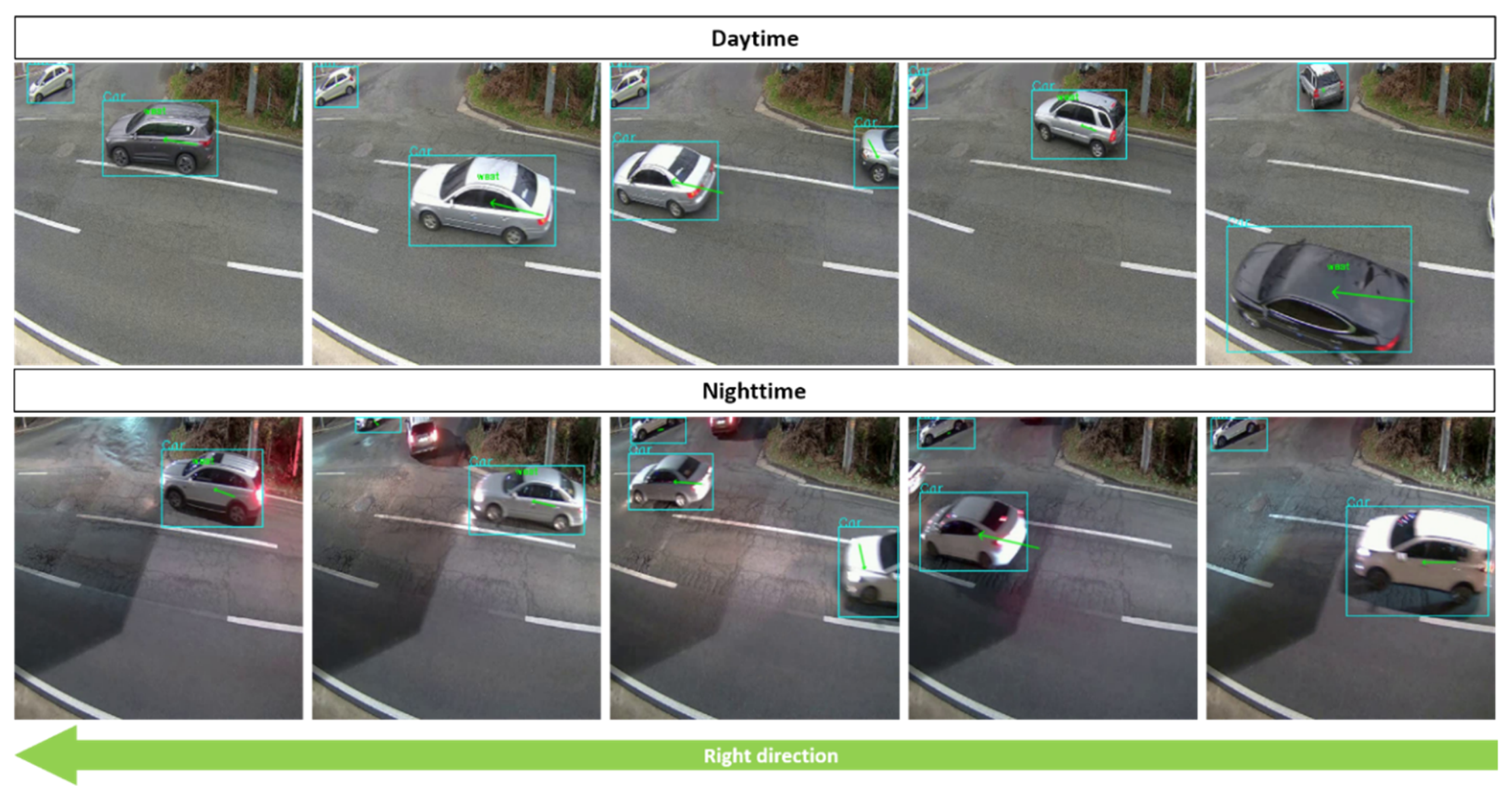
Due to safety reasons, Korean road traffic authority (KoROAD) did not allow us to simulate driving during nighttime. Therefore, for the second and third simulation cases we inverted daytime and nighttime videos as shown in
Figure 8 to check true-positive results. Results obtained from the first simulation case can be seen in
Table 2 where ‘positive direction’ is the number of cars moving in the correct direction, and ‘negative direction’ is the number of wrong-way driving cases. For case 1 we considered the case when the car was driven wrong-way in the daytime, where N is the total number of unique cars. For case 2 we considered a horizontally flipped video from case 1 and finally for the third case we took a flipped nighttime video to check the accuracy during nighttime. The reason we flipped the video frame is that Monteiro et al. [
8] used the image flipping method to check the accuracy of their system. From
Table 2 we can measure the performance of our wrong-direction detection system (
Table 3). Visual results are presented in
Figure 8.
Another evaluation we conducted determined false-positive results. The system was tested for 24 h to identify the number of false-positives. Our program counted 5552 cars passing by the camera within 24 h, identifying only one false-positive that occurred owing to the car’s illumination at night (
Table 4). Visual results on determining false-positive cases can be seen on
Figure 9.
5. Conclusions and Future Work
We propose a combined state-of-the-art YOLOv3 method with an updated linear quadratic equation to detect and track vehicles. To identify vehicles traveling in the wrong direction, we contributed a unique “entry-exit” method; and for simulation, in the three cases, we achieved an averaged accuracy of 91.98% in wrong-direction detection results. This system, as shown by the results obtained from simulations, presents excellent performance under various lighting conditions, so we can implement the program with real-world cameras. The current system works at 30 fps and was implemented on one of the roads in South Korea as a part of ITS solutions. Despite the good performance, our next milestone is adding new detection features to our network. As we experimented, we found many cases where pedestrians crossed the road in a prohibited area, so the next step in our research is to add violation detection of jaywalking.
Author Contributions
S.U. contributed towards the detection and tracking code. S.U. also worked on background system checks by implementing other researchers’ works. S.U. worked on improvement parts as well as analysis of a system and performed experiments. S.B. provided the experiments by recording and making the result tables and made visualizations and figures for the paper. S.B. also worked on frame extractions and annotations. K.J.W. provided all the data we used in this research and found a place where we could test our system in real-time. K.J.W. was the motivator and provided guidance about the “entry-exit” approach for direction validations and gave practical advice throughout the whole research process. All authors have read and agreed to the published version of the manuscript.
Funding
This project received no external funding.
Acknowledgments
This work was supported by an Inha University research grant.
Conflicts of Interest
The authors declare they have no conflicts of interest.
References
- Guo, G.; Wang, H.; Bell, D.A.; Bi, Y.; Greer, K. KNN Model-Based Approach in Classification. In Lecture Notes in Computer Science, Proceedings of the OTM: OTM Confederated International Conferences “On the Move to Meaningful Internet Systems”, Sicily, Italy, 3–7 November 2003; Springer: Berlin/Heidelberg, Germany, 2003. [Google Scholar] [CrossRef]
- Zivkovic, Z.; Van Der Heijden, F. Efficient adaptive density estimation per image pixel for the task of background subtraction. Pattern Recognit. Lett. 2006, 27, 773–780. [Google Scholar] [CrossRef]
- Zivkovic, Z. Improved adaptive gaussian mixture model for background subtraction. In Proceedings of the 17th International Conference on Pattern Recognition 2004. ICPR 2004, Cambridge, UK, 26–26 August 2004; Volume 2, pp. 28–31. [Google Scholar]
- Lucas, B.D.; Kanade, T. An iterative image registration technique with an application to stereo vision. Proc. Imaging Underst. Workshop 1981, 1981, 121–130. [Google Scholar]
- Shi, J.; Tomasi, C. Good features to track. In Proceedings of the Conference on Computer Vision and Pattern Recognition, Seattle, WA, USA, 21–23 June 1994; pp. 593–600. [Google Scholar]
- Tomasi, C.; Kanade, T. Detection and Tracking of Point Features. In Carnegie Mellon University Technical Report CMU-CS-91-132; School of Computer Science, Carnegie Mellon University: Pittsburgh, PA, USA, 1991. [Google Scholar]
- Barron, J.L.; Fleet, D.J.; Beauchemin, S. Performance of optical flow techniques. Int. J. Comput. Vis. 1994, 12, 43–77. [Google Scholar] [CrossRef]
- Monteiro, G.; Ribeiro, M.; Marcos, J.; Batista, J. Wrong-way Drivers Detection Based on Optical Flow. In Proceedings of the 2017 IEEE International Conference on Image Processing, San Antonio, TX, USA, 16 September–19 October 2007; pp. V-141–V-144. [Google Scholar] [CrossRef]
- Bouwmans, T.; Baf, F.E.; Vachon, B. Background Modeling Using Mixture of Gaussians for Foreground Detection—A Survey; Recent Patents on Computer Science; Bentham Science Publishers: Shaka, UAE, 2008; Volume 1, pp. 219–237. [Google Scholar]
- Liu, W.; Anguelov, D.; Erhan, D.; Szegedy, C.; Reed, S.; Fu, C.; Berg, A.C. SSD: Single Shot MultiBox Detector. arXiv 2016, arXiv:1512.02325. [Google Scholar]
- Ren, S.; He, K.; Girshick, R.; Sun, J. Faster R-CNN: Towards Real-Time Object Detection with Region Proposal Networks. arXiv 2015, arXiv:1506.01497. [Google Scholar] [CrossRef] [PubMed]
- Redmon, J.; Divvala, S.; Girshick, R.; Farhadi, A. You Only Look Once: Unified, Real-Time Object Detection. arXiv 2015, arXiv:1506.02640. [Google Scholar]
- Redmon, J.; Farhadi, A. YOLOv3: An Incremental Improvement. arXiv 2018, arXiv:1804.02767v1. [Google Scholar]
- Ambardekar, A.; Nicolescu, M.; Bebis, G. Efficient vehicle tracking and classification for an automated traffic surveillance system. Signal Image Process. 2008, 623, 101. [Google Scholar]
- Kanhere, N.K.; Birchfield, S.T.; Sarasua, W.A. Vehicle Segmentation and Tracking in the Presence of Occlusions. Transp. Res. Board Annu. Meet. 2006, 1944, 89–97. [Google Scholar] [CrossRef]
- Kuhn, H.W. The Hungarian Method for the assignment problem. Naval Res. Logist. Q. 1955, 2, 83–97. [Google Scholar] [CrossRef]
- Welch, G.; Bishop, G. An Introduction to the Kalman Filter. Special Interest Group on Computer Graphics and Interactive Techniques. 2001. Available online: https://www.cs.unc.edu/~tracker/media/pdf/SIGGRAPH2001_CoursePack_08.pdf (accessed on 14 January 2020).
- Tzutalin. LabelImg. Git Code. 2015. Available online: https://github.com/tzutalin/labelImg (accessed on 30 January 2020).
© 2020 by the authors. Licensee MDPI, Basel, Switzerland. This article is an open access article distributed under the terms and conditions of the Creative Commons Attribution (CC BY) license (http://creativecommons.org/licenses/by/4.0/).


