1. Introduction
As people’s living standards are improving increasingly, urban household and solid waste are also increasing greatly, which puts forward higher requirements for waste collection, transportation, and management. It also makes it difficult to collect, classify, transport and dispose of waste. Improper disposal can affect the urban landscape, occupy the land, pollute soil, pollute groundwater resources, affect air quality, spread diseases and affect environmental health and the health of residents. The cost of collecting and transporting urban household waste accounts for a large proportion of the total cost of the waste disposal system.
Our primary task is to solve waste collection problems. It is of great practical significance to analyze and study the path optimization of automatic collection and vehicles for reducing waste disposal costs and increasing waste disposal speed. The vehicle routing problem (VRP) has been an open problem and the front of operational research and combinatorial optimization. As a variation of VRP, the multi-depot vehicle routing problem (MDVRP) has also attracted more attention from scholars. The MDVRP problem is to allocate customers with the demand to each depot under the condition that the supply of each depot is not be exceeded and arrange the order in which customers are visited by vehicles. The objective function is to minimize the total route length and the number of vehicles.
Many heuristic algorithms have been applied to MDVRP. Heuristic algorithms are grouped in two as classical heuristics and modern metaheuristics. Since results obtained by heuristic algorithms are good in large scale problems, metaheuristic algorithms are used mostly in literature for types of the MDVRP.
Ant colony optimization (ACO) is a relatively new optimization method proposed by Dorigo et al. [
1]. Ant Colony Optimization algorithms, inspired by the phenomenon that ants would find the closet route to search for food, which belongs to the class of metaheuristics, are used exhaustively in the literature for MDVRP and its variants. ACO includes many algorithms which are many diverse variants of the basic principle. Demirel and Yilmaz [
2] proposed an approach based on ACO to solve MDVRP. Yu et al. [
3] presented a parallel improved ACO with a coarse-grain parallel strategy, ant-weight strategy and mutation operation for MDVRP. Stodola [
4] dealt with the modified MDVRP (M-MDVRP) which altered the optimization criterion. The optimization criterion of the standard MDVRP is to minimize the total sum of routes of all vehicles, whereas the criterion of M-MDVRP is to minimize the longest route of all vehicles, i.e., the time traveled by the vehicle is as short as possible. For this problem, they also developed a metaheuristic algorithm based on the Ant Colony Optimization theory to solve the classic MDVRP instances—this has been modified and adapted for M-MDVRP. They also proposed an additional deterministic optimization process which further enhances the original ACO algorithm. They used Cordeau’s benchmark instances to evaluate results. Some articles [
5,
6,
7] adopted ACO to solve the variants of MDVRP, such as MDVRP with multiple objectives and MDVRP with time windows.
The genetic algorithm also belongs to a class of metaheuristics. Ho et al. [
8] developed two hybrid genetic algorithms (HGAs). In HGA1, the initialization procedure is conducted randomly. HGA2 incorporated the Clarke and Wright saving method and the nearest heuristic neighbor to generate initial solutions. Based on a computational study, they compared the performance of the algorithms with different problem sizes. It is proven that the performance of HGA2 is superior to that of HGA1 in terms of the total delivery time. Dantzig and Ramser [
9] adopted a phased aggregation strategy to solve the VRP with the homogeneous trucks. Clarke and Wright [
10] considered multiple truck capacity as a further formulation. They proposed a saving method which may be readily performed and very fast in a computer application. This method is the famous Clarke and Wright Saving (CWS) method mentioned earlier. Ho et al. adopted CWS to solve single VRP, however, we decomposed the VRP into several Travelling Salesman Problems (TSPs) [
11] and solved them respectively using CWS. For the TSP, the CWS released the vehicle capacity restriction, which can be performed easily and get near-optimal results quickly. Karakatič and Podgorelec [
12] presented a survey of genetic algorithms that are designed for solving MDVRP. Besides providing an up-to-date overview of the research that focuses on different genetic approaches, methods, and operators used in selection, crossover, and mutation, the results of a thorough experiment are presented and discussed, which evaluated the efficiency of different existing genetic methods on standard benchmark problems in detail. The specific methods, operators and settings are presented to help researchers and practitioners to optimize their solutions in further studies.
Most of the papers adopted the local search algorithm. The local search algorithm is improved from the hill-climbing algorithm. The local search algorithm is simply a greedy search algorithm, which selects the best neighbor from the neighborhood of the current solution as the current solution of the next iteration until a local optimal solution is reached. Juan et al. [
13] employed two biased-randomized processes that relied on the use of the geometric probability distribution at different stages of the iterated local search (ILS) framework to solve MDVRP. The first process is assigning customers to depots using a randomized priority criterion and another is improving routing solutions associated with a “promising” allocation map. It is relatively easy to implement and can be parallelized in a very natural way. Li et al. [
14] solved the MDVRP with simultaneous deliveries and pickups (MDVRPSDP) and put an adaptive neighborhood selection mechanism that employs a scoring rule into the improvement steps and the perturbation steps of iterated local search, respectively. They also proposed new perturbation operators to diversify the search. Ahmadi [
15] devised a variable neighborhood search algorithm to solve the deterministic MDVRP model to facilitate humanitarian logistics operations. Alinaghian and Shokouhi [
16] developed a hybrid algorithm composed of an adaptive large neighborhood search and variable neighborhood search to solve this problem in which the cargo space of each vehicle has multiple compartments, and each compartment is dedicated to a single type of product. Ahmadi Vidal et al. [
17] combined a genetic algorithm with neighborhood selection mechanisms to manage diversity for a large class of vehicle routing problems with time-windows.
The traditional MDVRP has often been studied mainly with a focus on economic benefits. In recent years, the growing concern about the effects of pollutions has forced researchers to address the socio-environmental concerns. Du et al. [
18] considered minimizing the total transportation risk as to the objective function and proposed a fuzzy bilevel programming model to solve the problem of transporting hazardous materials from multiple depots to customers. They introduced a numerical, integration-based fuzzy simulation method combined with four heuristic algorithms (hybrid particle swarm optimization, genetic algorithm, ant colony algorithm, and simulated annealing algorithm) to find the optimal solutions assigning customers to depots and determining the best paths regarding each group of depots and customers. Illustrative examples showed the good performance of the proposed model and the four heuristics. Oliveira et al. [
19] proposed a cooperative coevolutionary algorithm which decomposed the MDVRP into some subproblems, that is, single depot VRPs which evolve separately. However, the quality of a solution depends on a good complete solution formed by one solution obtained by an individual cooperated with partial solutions from other populations. The introduced approach performed very well in parallel environments. Therefore, they applied a variable-length genotype coupled with local search operators in a parallel evolution strategy environment and conducted a large number of experiments to assess the performance of this approach. The results suggest that the proposed coevolutionary algorithm in a parallel environment can produce high-quality solutions to the MDVRP in low computational time. Jabir et al. [
7] focused on economic cost and emission cost reduction for a capacitated multi-depot green vehicle routing problem. They formulated an integer linear programming model for solving a set of small-scale instances using the LINGO solver and developed a computationally efficient Ant Colony Optimization based meta-heuristic for solving both small scale and large scale problem instances in a reasonable amount of time. The latter algorithm’s performance is improved by integrating it with a variable neighborhood search.
Considering the future when everything is connected, product logistics routing requires faster response times. This paper aims to get better solutions quickly to respond to changes in requirements from customer and market demands. Compared to the existing approaches, we address single depot VRP in parallel and inevitably gave up pursuing the best solution.
In our study, after assigning waste collection points to waste disposal plants, each depot solves the VRP, assigning customers to vehicles and planning the order in which customers are visited by the vehicles. This process can be parallelized. The sector combination optimization (SCO) algorithm is used to generate multiple initial solutions, with these solutions as the initial population of genetic algorithm or ant colony optimization algorithm, the number of iterations can be reduced to achieve fast convergence. Additionally, because of the abundant initial solutions, the algorithm can avoid trapping in a local optimum. Then these initial solutions are improved using the merge-head and drop-tail (MHDT) strategy. After a certain number of iterations, the optimal solution in the last generation is reported.
The paper is structured as follows. In
Section 2, we give a detailed description of the sector combination optimization algorithm.
Section 3 explains the merge-head and drop-tail strategy. Experimental results on the benchmark instances are reported in
Section 4. Finally, conclusions and some potential directions for future research are presented in
Section 5.
2. The Sector Combination Optimization Algorithm to Obtain Initial Solutions
The above waste collection problem can be modeled as MDVRP. MDVRP can be defined as follows based on [
20]: Let
denotes a graph where V represents a collection of points and E represents a collection of edges. V can be divided into two parts:
represents a group of customers, N is the number of customers;
represents a group of depots, M is the number of depots. Each customer has a non-negative demand
; each arc belonging to E has an associated cost
, and the cost in this article is distance. K denotes the number of vehicles owned by each depot and
indicates the capacity of the vehicle.
is the decision variable as shown in Equation (1).
Conditions:
- (1)
The number of depots and customers and the location of their coordinates are predetermined.
- (2)
The customer’s demand and vehicle capacity are known.
Constraints:
- (1)
Each route starts and ends at the same depot.
- (2)
The total demand of the customers on each route does not exceed the vehicle capacity.
- (3)
Each customer is served by one vehicle and is served only once.
To understand the algorithm clearly, an MDVRP example shown in
Figure 1 is proposed.
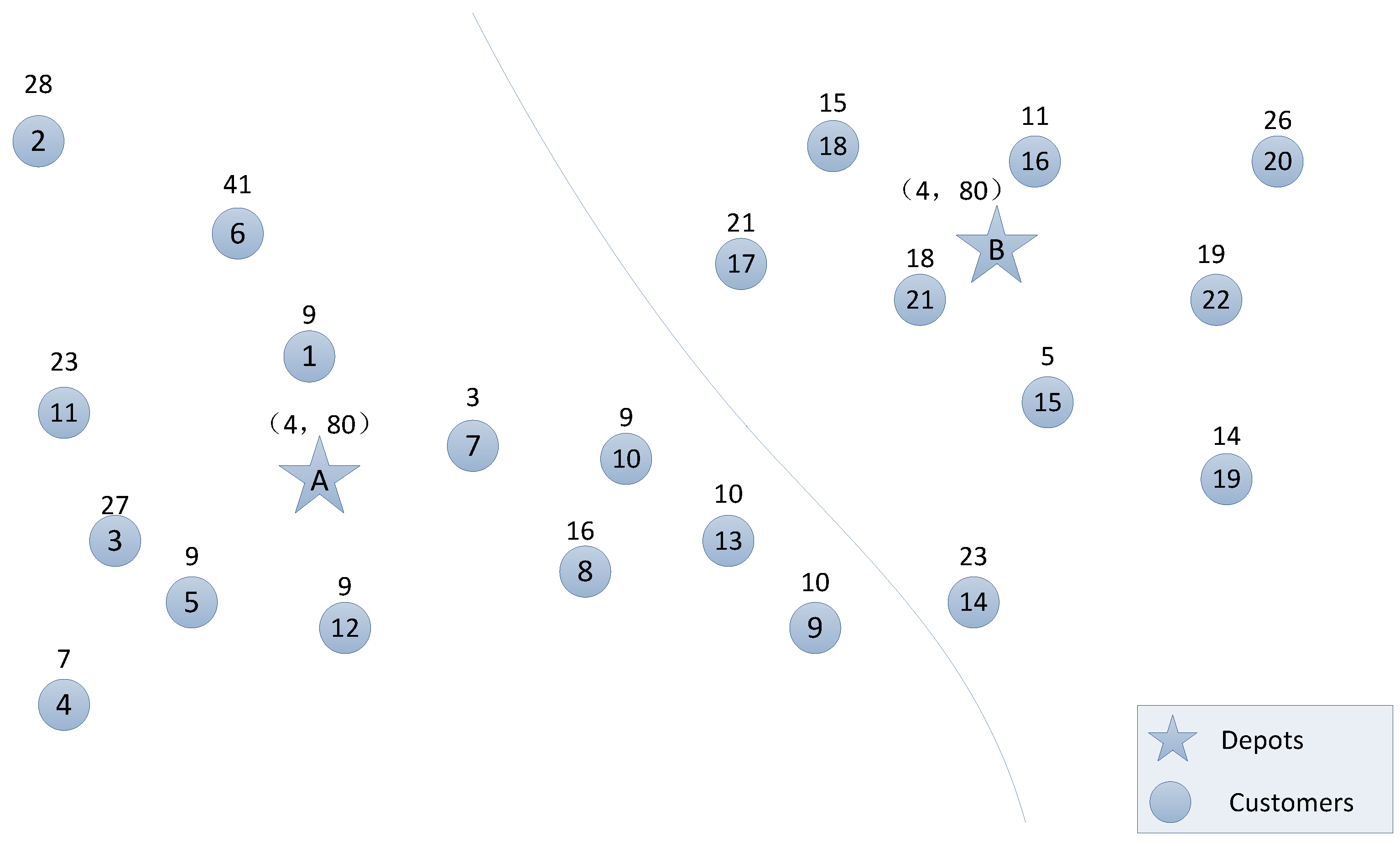
Figure 1 is a graph with 24 points, where 22 points represent customers and two points represent depots. In the figure, the circle represents the customer and the square represents the depot. The coordinates of the depot and the customer are predetermined, the customer’s demand is shown above the customer point, the first value in the brackets above the depot represents the number of vehicles and the second value represents the vehicle capacity.
In the Equation (3),
represents the total customer demand of the depot D,
represents the total supply of depot D. In the constraint that the total customer demand does not exceed the total supply in each depot, the customer will be assigned to each depot according to the nearest distance, and the vehicle routing problem (VRP) for each depot will be solved simultaneously.
Taking the MDVRP problem into consideration, the assignment result is shown in
Figure 1. The customer number assigned to the A depot is 1-2-3-4-5-6-7-8-9-10-11-12-13, and the customer number assigned to the B depot is 14-15-16-17-18-19-20-21-22. Next, to solve the VRP in each depot.
2.1. Group the Customers
Group the customers into two parts according to the nearest distance from the depot under the constraint (4), which is graphically like two concentric circles.
represents the total customer demand of the inner circle of depot D, and
represents the total customer demand of depot D.
The constraint (4) means that the total customer demand of the inner circle does not exceed half of the total supply of the depot D.
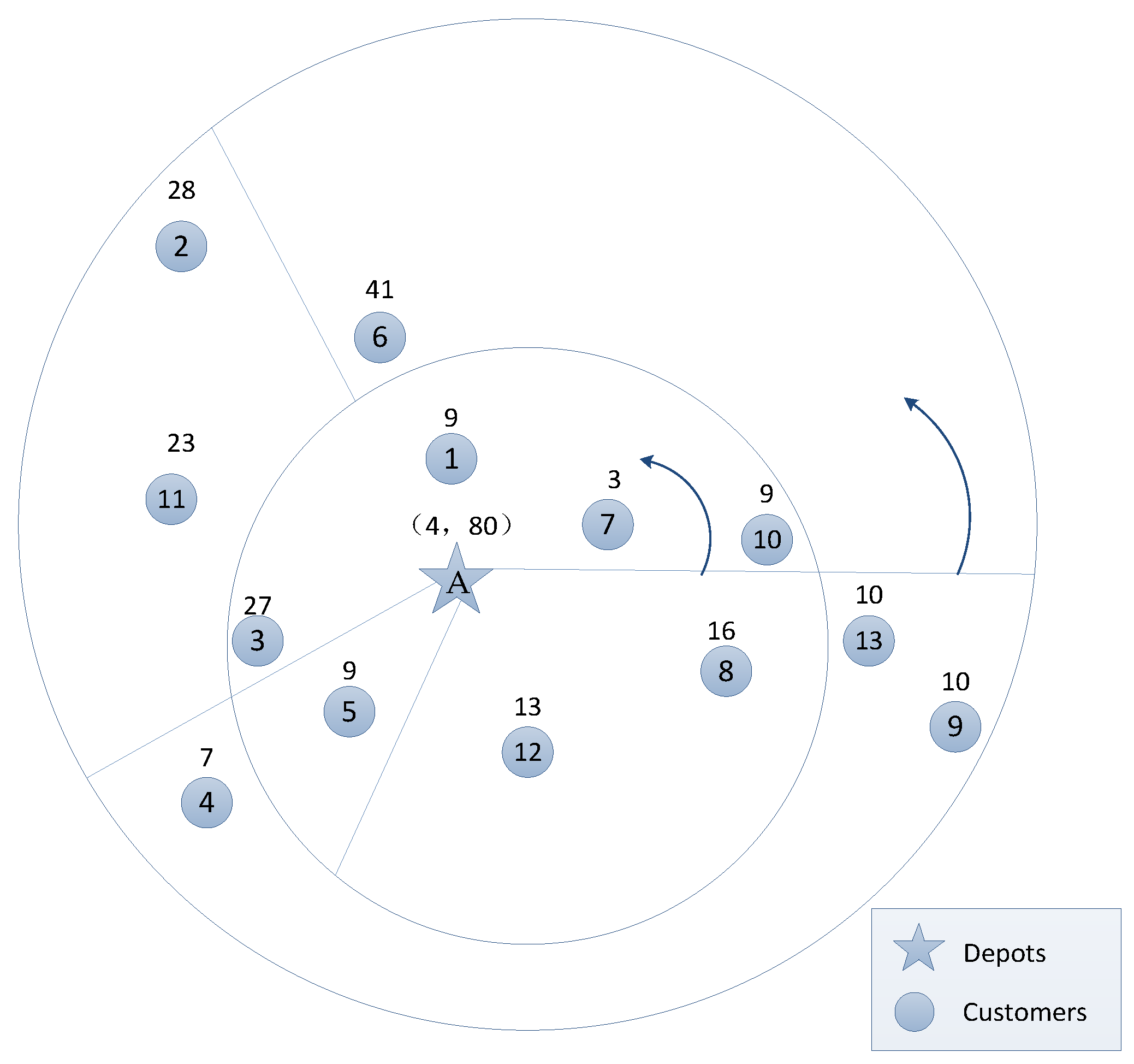
For depot A, the total customer demand is 205, and half of the total demand is 205/2 = 102.5. Therefore, according to the nearest distance, under the constraint that the total demand does not exceed 102.5, the customers are allocated to the inner circle, and the remaining customers are assigned to the outer circle. The result of the grouping is shown in
Figure 2. The customers belonging to the inner circle are: 1-3-5-7-8-10-12; the total customer demand of the inner circle is 86; the customers belonging to the outer circle are: 2-4-6-9-11-13, the total customer demand of the outer circle is 119.
2.2. Segment the Circle
Next, we segmented the circle forward based on the forward order of the customers’ polar coordinates. As a result, some customers have been grouped into one sector randomly.
In Equation (5),
S denotes the number of sectors that we need, [] indicates rounding up. Besides, if
S = 1, there is no need to cut the circle; if
S = 2, let
S = 3, this ensures that the polar forward and backward customers can be grouped. When cutting the circle, the random segmentation principle is adopted, but the total customer demand within each sector must not exceed the vehicle capacity.
in Equation (6) denotes the total customer demand within the sector Se.
The total customer demand of the depot A is 205 and the vehicle capacity is 80, therefore the number of sectors for the depot A is three. According to the forward order of the customer polar coordinate, the customers belonging to the inner and outer circle are randomly grouped into three sectors, respectively. The total customer demand within each sector does not exceed 80. A result of the segmentation is shown in
Figure 2. The arrows in the figure indicate the direction of segmentation. The sectors within the inner circle are: [10, 7, 1, 3], [5], [12, 8], the sectors within the outer circle sectors are: [6], [2, 11], [4, 9, 13].
2.3. Arrange the Sectors
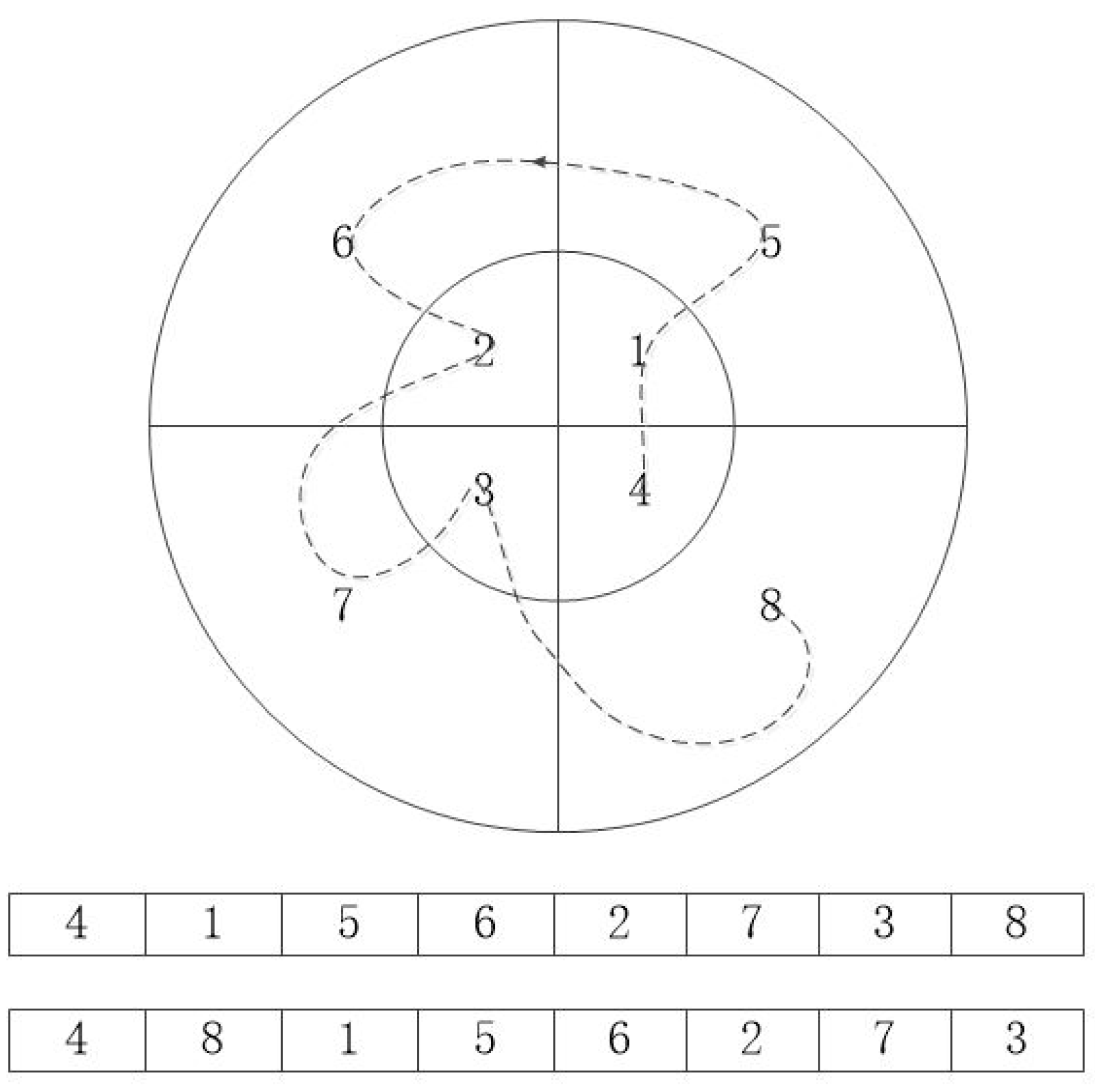
A sector in the inner or outer circle is randomly selected as the first sector, and its adjacent sectors within the inner and outer circle are sorted anticlockwise by a threading-needle method. The principle of the threading-needle method is that, except for the first sector, the remaining sectors within the inner circles must follow after the corresponding sectors within the outer circles. Similarly, the remaining sectors within the outer circles must follow after the corresponding sectors within the inner circles. That is, the sectors belonging to the inner circle must be together with their corresponding sectors belonging to the outer circle. The sector corresponding to the first sector can be arranged on the 2nd or the end.
As shown in
Figure 3, eight sectors belong to the inner or outer circle, and sector four within the inner circle is selected as the first sector, and the corresponding sector eight belonging to the outer circle is not selected as the second sector, it will be put at the end of the sequence. The threading-needle method is shown in
Figure 3, and the direction of the arrow is the direction of threading the needle. One result is the first sequence in
Figure 3. Similarly, sector four is selected as the first sector, and the sector eight is selected as the second sector. Consequently, one result is the second sequence in
Figure 3.
According to the above rules, a result of the sector arrangement of the depot A is shown in
Figure 4a. The sector sequence is: [12, 8], [4, 9, 13], [10, 7, 1, 3], [6], [2, 11], [5].
2.4. Group the Sectors
After obtaining the sector sequence, the sectors in the sector sequence need to be grouped and customers must be assigned to vehicles. Starting from the first sector of the obtained sector sequence, the sectors are grouped according to customer demand. The grouping rule is: if the total demand of customers in the current sector and its latter sector does not exceed the vehicle capacity, then the customers in the two sectors are allocated in the same vehicle, and the next sector is grouped similarly. Otherwise, the customer in the latter sector is added to the current sector in order; if the sum of the demand of one customer and the total customer demand of the current sector exceeds the vehicle capacity, skip this customer and select the next customer in the latter sector, and so on, maximizing the vehicle load without exceeding the vehicle capacity. The remaining customers in the latter sector are then grouped into one sector as the current sector, continuing to group its latter sector.
As shown in
Figure 4b, the total customer demand of the sector [12, 8] is 29.0, the total customer demand of the sector [4, 9, 13] is 27.0, and the sum of two sectors is 56.0, which does not exceed the vehicle capacity, 80.0. Therefore, the two sectors are grouped into one sector [12, 8, 4, 9, 13]. The total customer demand of the next sector [10, 7, 1, 3], 48.0, 56.0 + 48.0 = 104.0, exceeds the vehicle capacity, 80.0, so the customers in the sector [10, 7, 1, 3] are selected to add to the sector [12, 8, 4, 9, 13] in order. The result is that 10, 7, 1 have been added to the sector [12, 8, 4, 9, 13]; therefore, customers 12, 8, 4, 9 13, 10, 7, 1 are assigned to a vehicle and the sector [3] is left as the current sector, and so on. As a result, as shown in
Figure 4b, the customers 12, 8, 4, 9, 13, 10, 7, 1 are assigned to the first vehicle, and the customers 3 and 6 are assigned to the second vehicle, and the customers 2, 11, 5 are assigned to the third vehicle.
2.5. Arrange the Customers
At this point, the problem becomes a traveling salesman problem (TSP). We use the CWS method to rearrange the order in which customers are served.
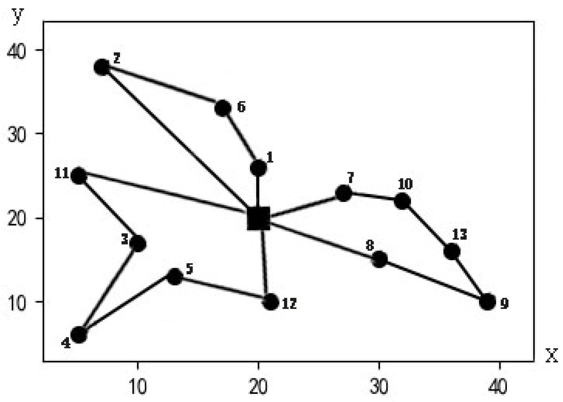
The result of the customers being serviced is shown in
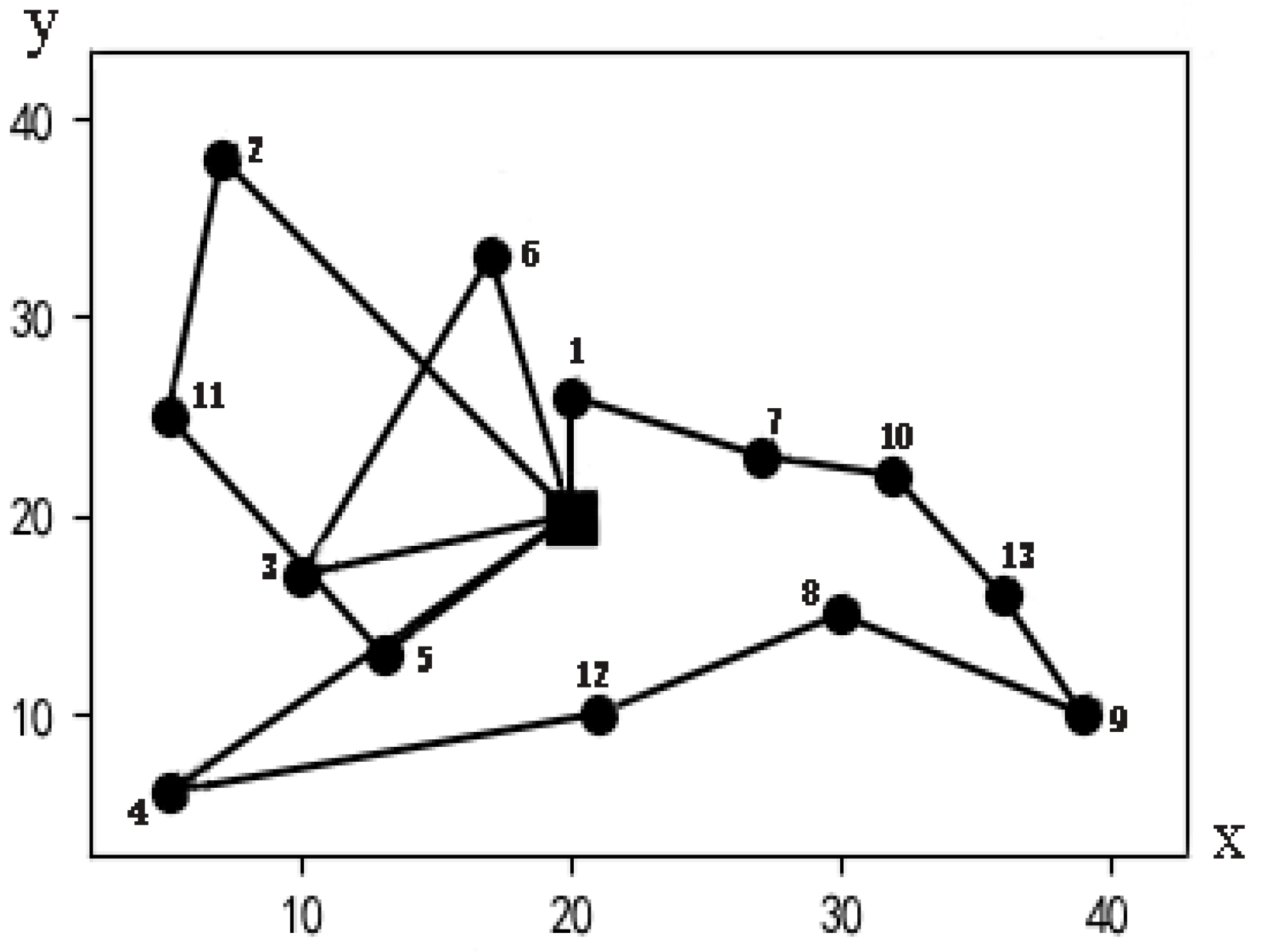
Figure 4c, the route of vehicle 1: 4-12-8-9-13-10-7-1, the route of vehicle 2: 3-6, and the route of vehicle 3: 2-11-5. The road map is shown in
Figure 5, the objective function value, that is, the total distance of the routes, 191.16.
3. The Merge-Head and Drop-Tail Strategy to Improve Initial Solutions
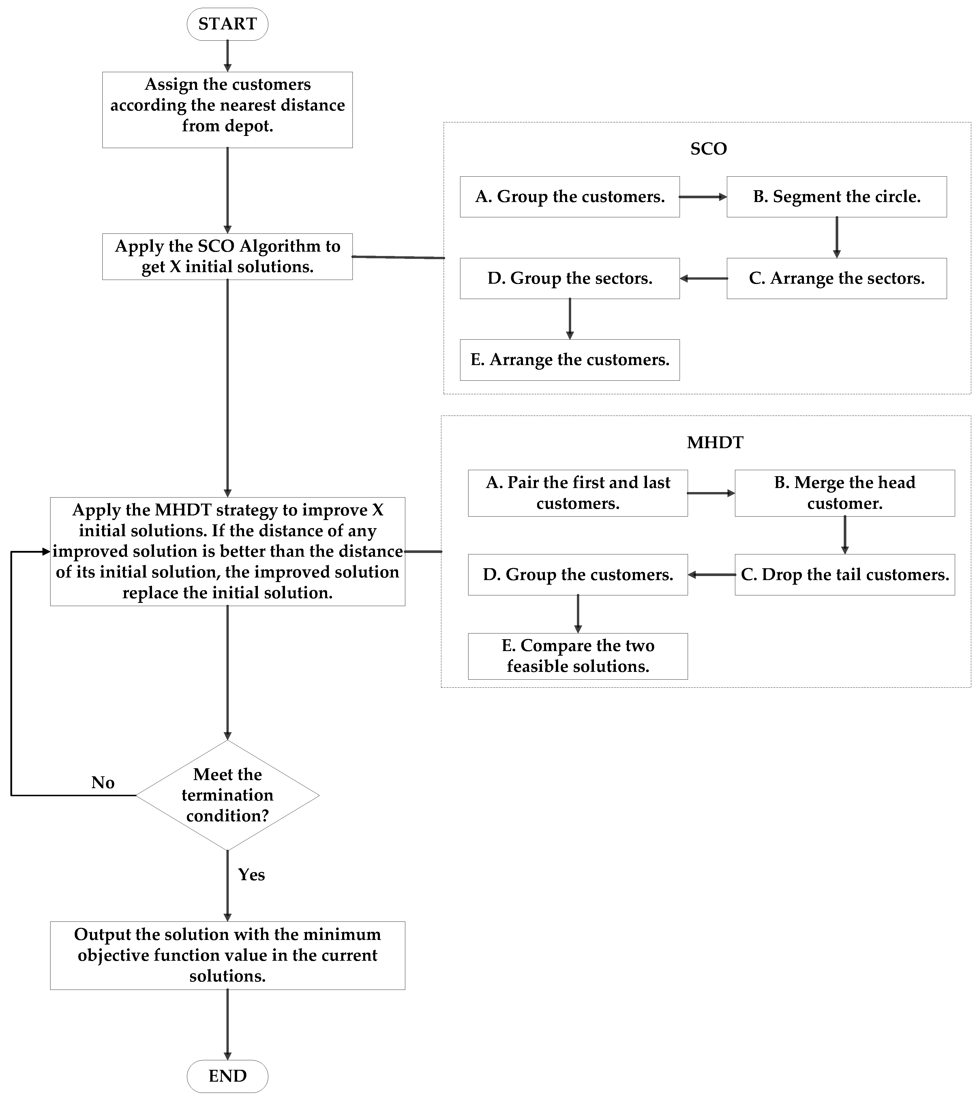
The X initial solutions obtained are selected for further optimization. If one improved solution is better than the initial solution, then the optimization is continued instead of the initial solution. The flowchart of the whole procedure is shown in
Figure 6.
3.1. Pair the First and Last Customers
Select the first (head) and last (tail) customers of each route, and pair the head (tail) customers of each vehicle with the first and last customers of other vehicles. Assuming the number of routes is R, the number of pairs is:
Then add all the pairs to the list, such as .
In
Figure 6, customers 4 and 1 of route 1, customers 3 and 6 of route 2, and customers 2 and 5 of route 3 need to be paired. Consequently, the list is: [[4, 3], [4, 6], [4, 2], [4, 5], [1, 3], [1, 6], [1, 2], [1, 5], [3, 2], [3, 5], [6, 2], [6, 5]], a total of [(3 − 1)^2 + (3 − 1)] × 2 = 12 pairs.
3.2. Merge the Head Customer
Next, the merging operation of the nearest customer pair on the list must be performed. The merging rule is that the later customer in the pair is added to the route of the vehicle where the previous customer is located, and another customer of the vehicle paired with other customers is recorded. Finally, the customers are rearranged with the CWS method and get the new customer sequence visited by the vehicle . The order of the two customers in the pair is switched and the merging operation on the new pair is performed.
The nearest customer pair in the initial solution shown in
Figure 5 is [3, 5]. Customer 5 is firstly added to the route in which customer 3 is located, that is, the route of the vehicle 2. The tail customer of the route is customer 6. A feasible improved solution after the CWS method is the route of the vehicle 1: 4-12-8-9-13-10-7-1, the route of the vehicle 2: 6-3-5, the route of the vehicle 3: 2-11. It can be easily computed that the total demand of the customers in vehicle 2 is 77.0, which does not exceed the vehicle capacity. The total distance of the new routes is 187.11.
Then, the order of the customers in the nearest customer pair is reversed, that is, [5, 3]. Similarly, customer 3 in the initial solution is added to the route in which customer 5 is located, that is, the route of vehicle 3. The tail customer of the route is customer 2. The current route is re-planned with the CWS method: the route of the vehicle 1: 4-12-8-9-13-10-7-1, the route of the vehicle 2: 6, the route of vehicle 3: 2-11-3-5.
The total demand of the customers in vehicle 3 is 87.0, which exceeds the vehicle capacity.
3.3. Drop the Tail Customers
It is judged whether the total demand of the customers in the vehicle to which the head customer is added is greater than the vehicle capacity, and if it is greater than the vehicle capacity, the customers in the current vehicle need to be dropped. The dropping rule is: judge the position of another customer in the current vehicle recorded in step B in the new customer order, if it is before 1/2 of the current order (including 1/2), then starting from the first customer, drop the customers visited by the current vehicle until the limit about the vehicle capacity cannot be met; otherwise, drop the customers from the last customer. Record the customers that need to be dropped in turn, that is, and put them into one sequence .
It is judged above that the total demand of the customers in vehicle 3 is 87.0, which exceeds 7.0, compared with the vehicle capacity. Therefore, the tail customers need to be discarded, and the position of customer 2 in the route of vehicle 3 is judged to be No.1, before the 1/2 of the customer order, so the first customer of the vehicle 3 (still the customer 2) is selected for dropping. Customer 2 has a capacity of 28.0, which is greater than 7.0, so only dropping customer 2 is enough.
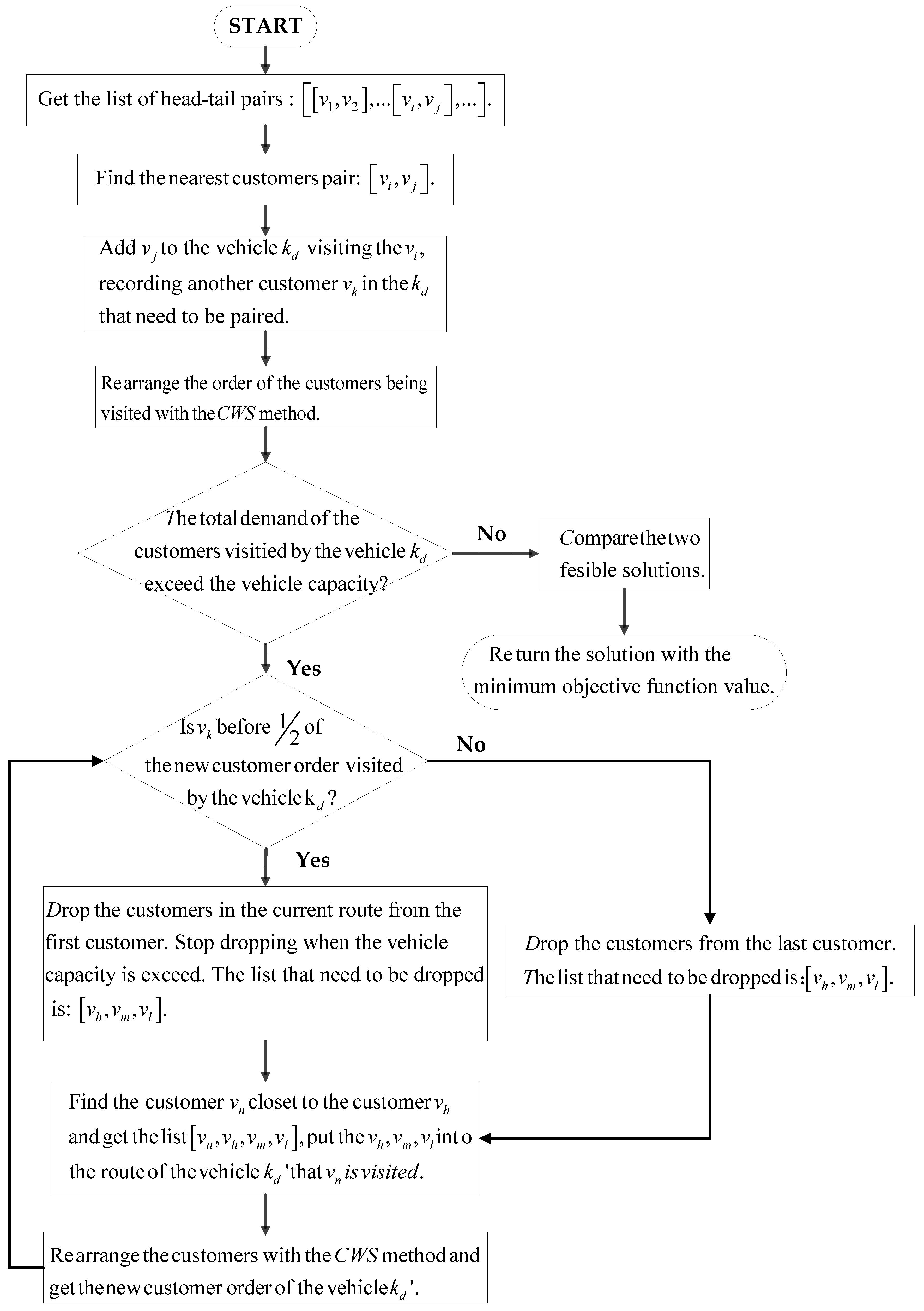
3.4. Group the Customers
Find the customer
in the first and last customers in the vehicles except for the vehicle
is closest to the first customer
in the sequence
. Put the customer
on the first position of the sequence. Go back to step B, the later customers
in the sequence is added to the route of the vehicle
where the previous customer
located, and another customer
of the vehicle
paired with other customers is recorded, and so on, for the next step. Specific steps can be seen in
Figure 7.
The customer in the first and last customers in the other vehicles closest to customer 2 is 6. A sequence [6, 2] is formed, and customer 2 is added to the route of vehicle 2 where customer 6 is served. A new feasible and improved solution is the route of the vehicle 1: 4-12-8-9-13-10-7-1, the route of vehicle 2: 6-2, the route of vehicle 3: 11-3-5. The total customer demand for vehicle 2 satisfies the limit of the vehicle capacity, and the total distance is 177.11.
3.5. Compare Two Feasible Solutions
The solution with the smaller objective function value is compared with the initial solution: if it is smaller than the initial solution, the solution replaces the initial solution to be added to the X initial solutions. If the number of iterations is not reached, the X initial solutions return to step A to be optimized again; otherwise, output the solution with the minimum objective function value in the current solutions.
The objective function value of the first improved solution is 187.11 and the second one is 177.11. The second solution is smaller than the first solution and is better than the initial solution. Therefore, the solution replaces the initial solution, and returns to Step A. After 30 iterations, the road map of the final solution is shown in
Figure 8.
4. Computational Experiments
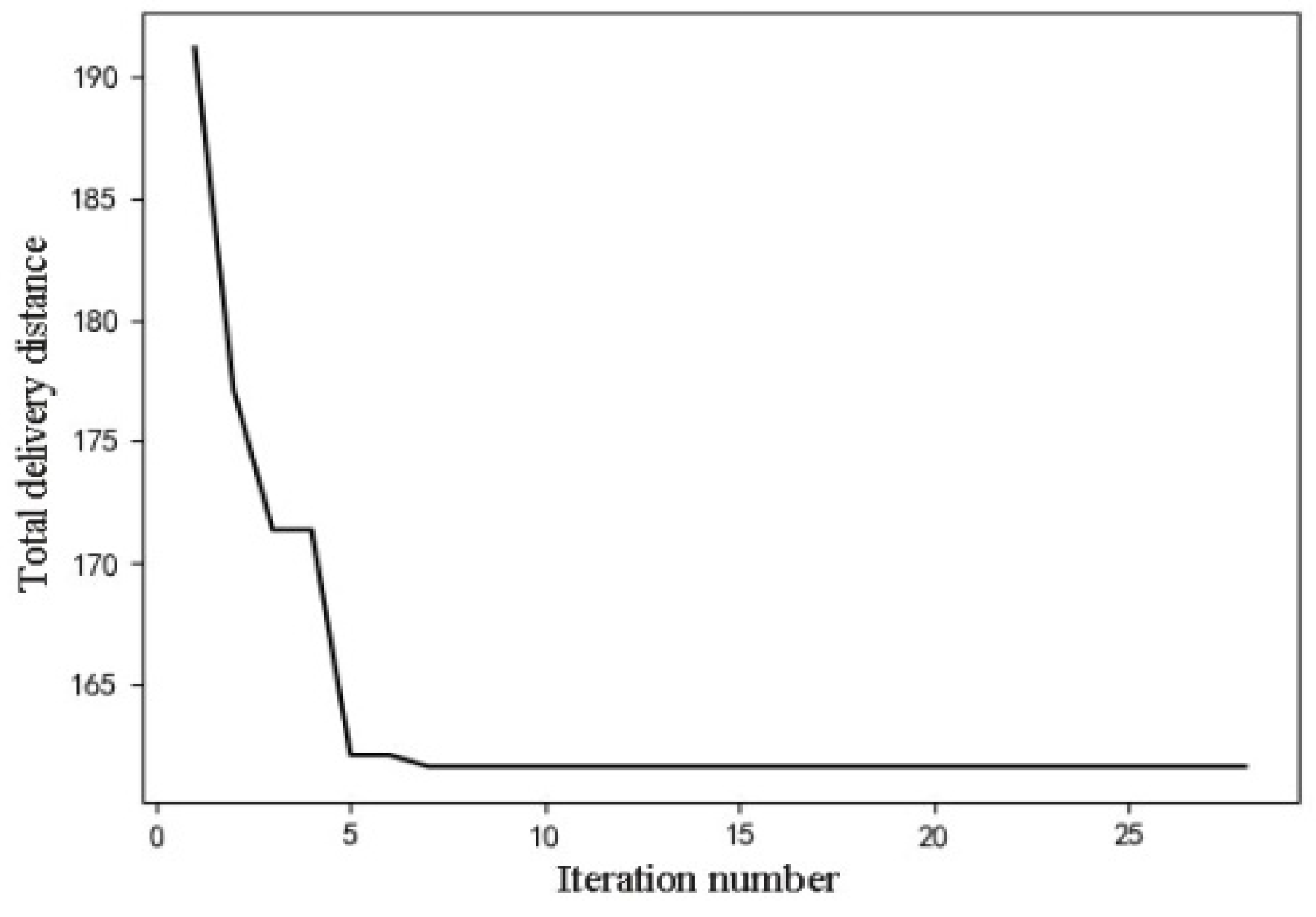
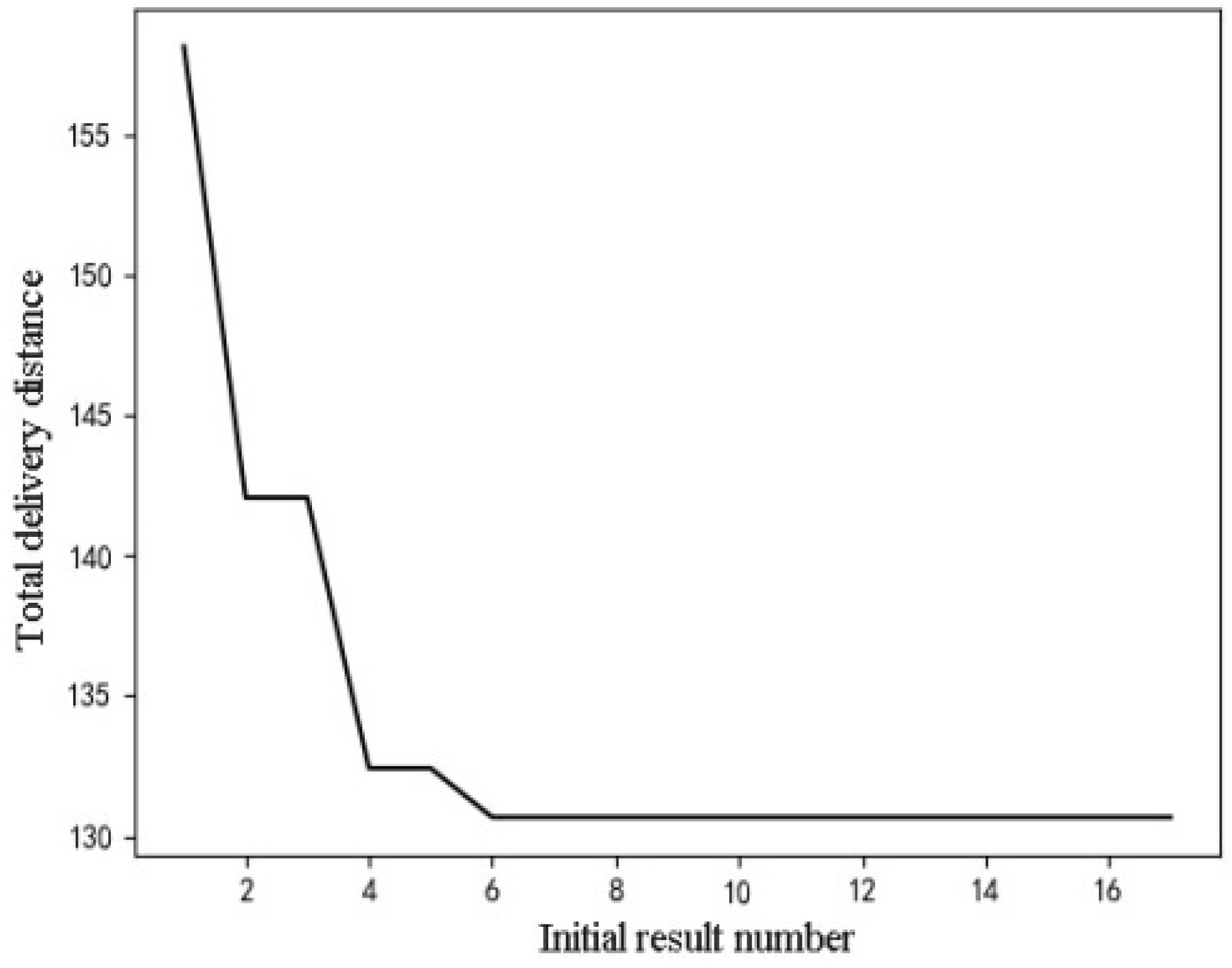
The iteration curve of depot A is shown in
Figure 9. Compared with the initial solution, after 30 iterations, the objective function of the final solution is reduced by 29.5 and has converged at the 8th iteration. The iteration curve of depot B is shown in
Figure 10. After 18 iterations, the final solution reduces the distance of 27.44 compared with the initial solution. The curve has converged at the 6th iteration. It can be seen that the merge-head and drop-tail strategy improves the initial solution quickly, and the number of iterations is small so that a better solution can be obtained quickly.
Considering 23 benchmark instances proposed for the MDVRP, the performance of the sector combination optimization algorithm and the merge-head and drop-tail optimization strategy are shown in
Table 1. The experiment was implemented in Python, on Intel(R) Core(TM) i5-4260(U) CPU @ 1.40 GHz (manufacturer: Apple Inc., Cupertino, California, USA).
In
Table 1, for each instance, the meaning of the notation is provided at the end of this paper.
In
Table 1, for each instance, the parameters in
Table 2 are used. Taking the instance 1 as an example, it has 50 customers and four depots, and each depot has four vehicles with a capacity of 80. We adopt the SCO algorithm to get 30 initial solutions and improve these 30 solutions by the MHDT algorithm until the ending criterion, namely 20 iterations, is met.
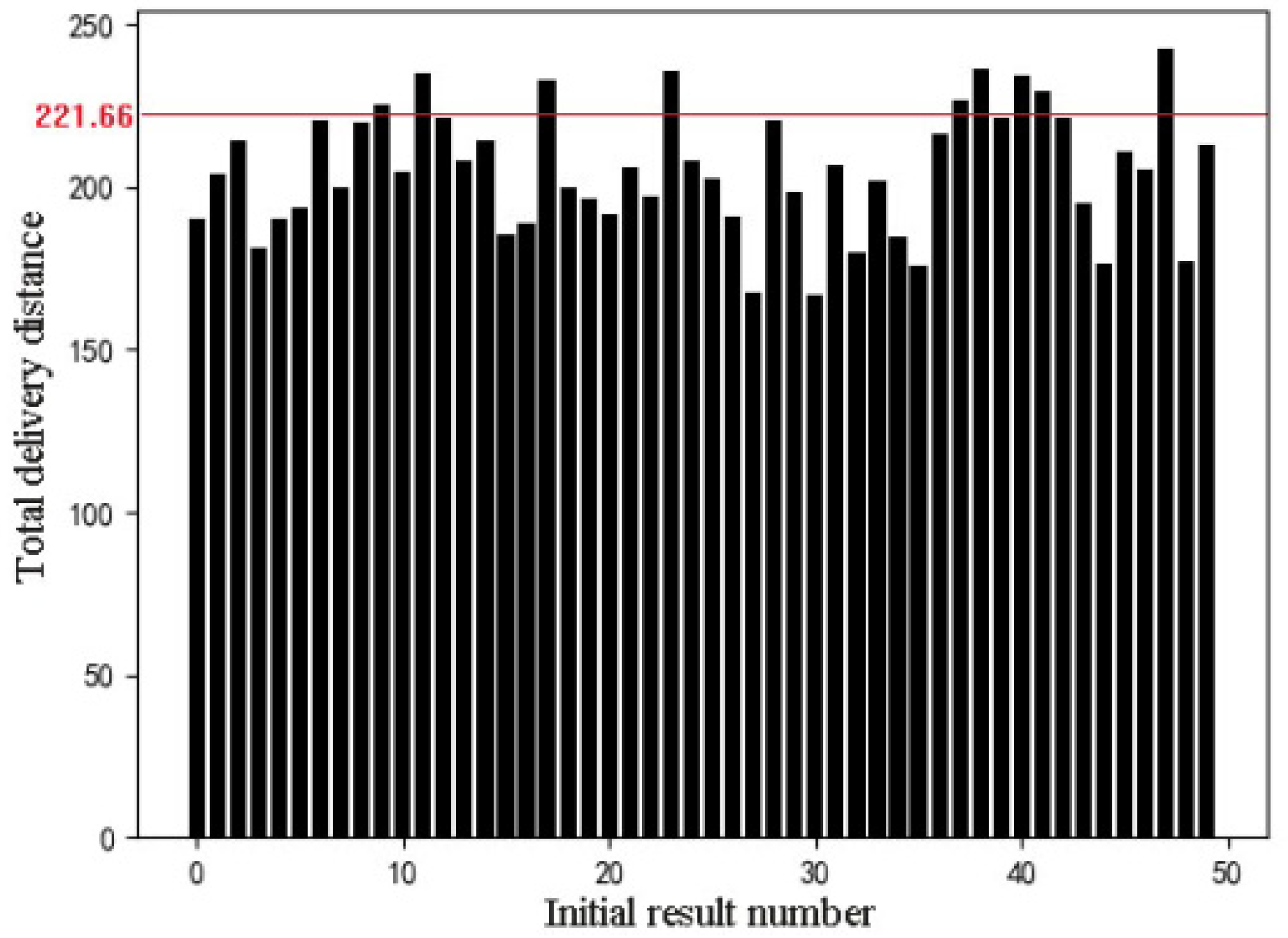
The sector combination optimization algorithm makes the initial solutions more abundant and better, compared with other iterative algorithms only using one initial solution such as the genetic algorithm adopted by Ho et al. [
8] and granular Tabu search algorithm adopted by Escobar et al. [
21]. Ho et al. adopted the CWS method to get a solution for initialization. For the small problem with 13 customers, the objective function value of the solution obtained by CWS is 221.66, and the objective function values of 50 initial solutions obtained by the sector combination optimization algorithm fluctuate between 150 and 250, of which 82% is below 221.66, as shown in
Figure 11. For the two depots with 249 customers of the instance 8, as shown in
Table 1, the objective function value of the solution obtained by CWS is 4671.2, and the objective function values of 50 initial solutions obtained by the sector combination optimization algorithm fluctuate between 2500 and 3500, of which 100% are below 4671.2. It can be seen that the initial solution obtained by the sector combination optimization algorithm is better. With these solutions as the initial population of the genetic algorithm and ant colony algorithm, the number of iterations can be reduced to achieve fast convergence. Additionally, because of the abundant initial solutions, the algorithm can avoid trapping in a local optimum.
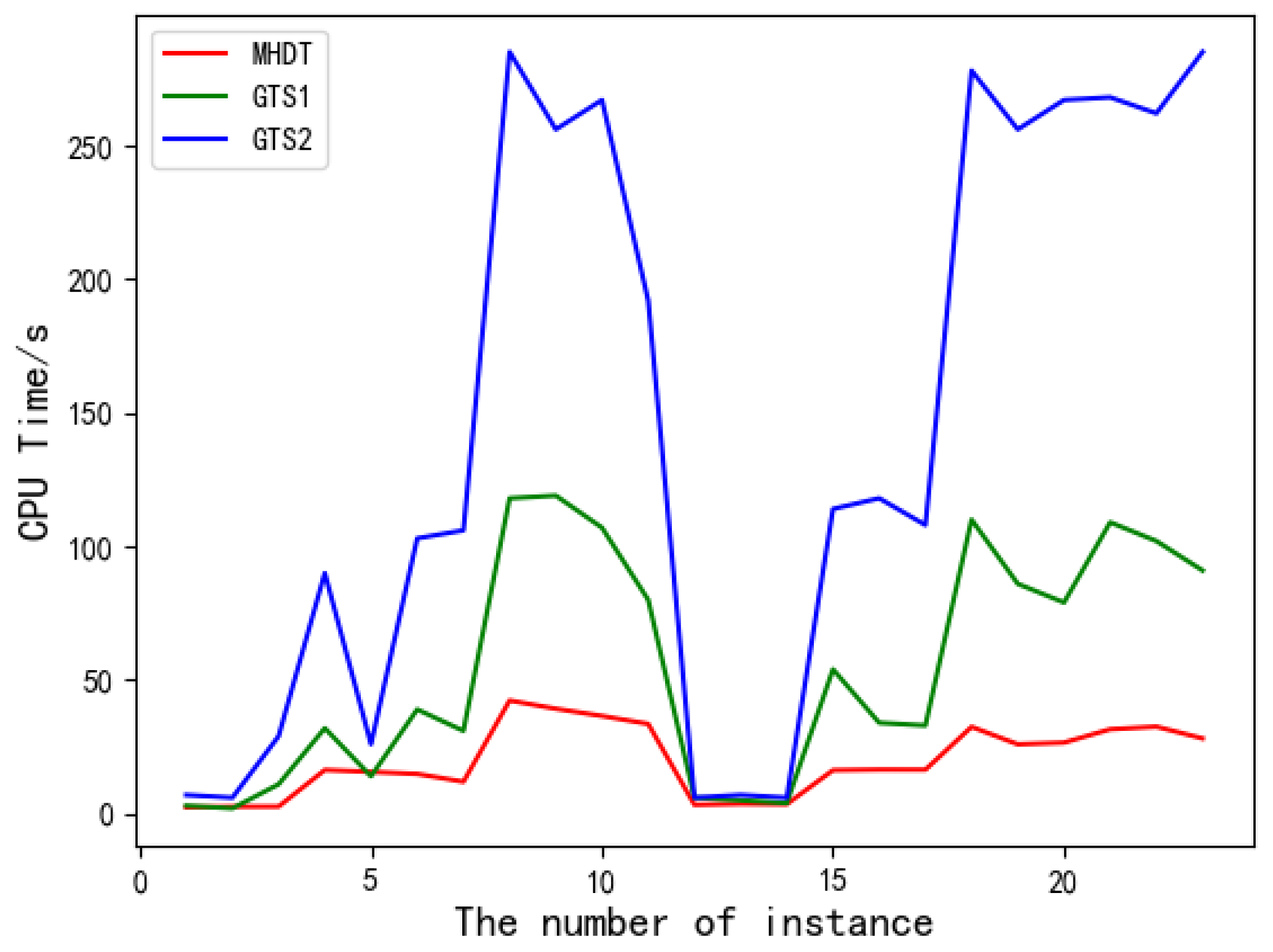
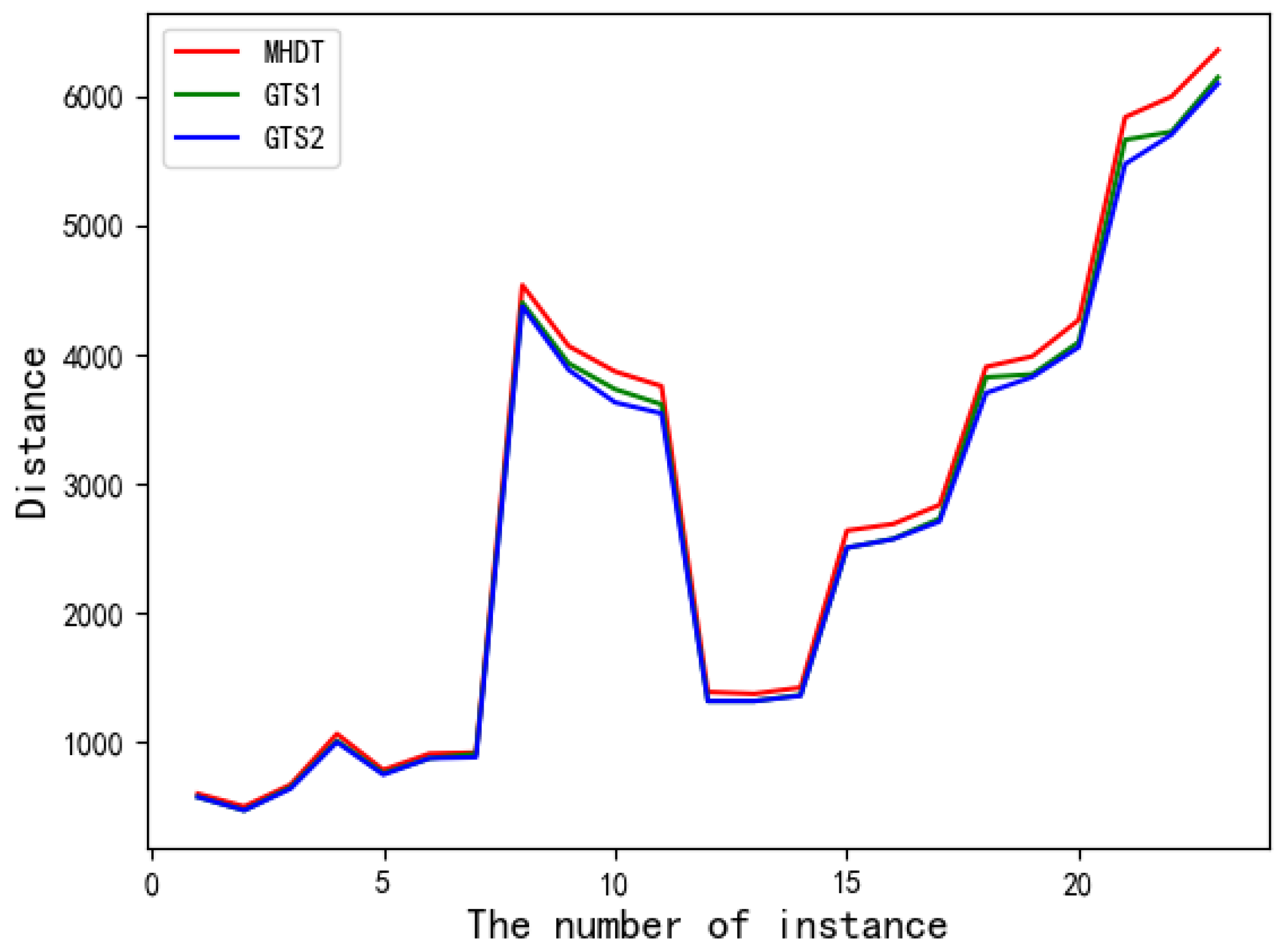
Escobar et al. proposed a hybrid granular Tabu search (GTS) algorithm for the MDVRP based on a cluster approach like our algorithm while they aimed to find the best solutions. The initial MDVRP solution is obtained by using a hybrid initial procedure (GTS1) and improved by the granular Tabu search procedure (GTS2). We illustrate the performance of the two algorithms in terms of CPU time and distance for comparisons. Combing
Figure 12 with
Figure 13, we conclude that the CPU time consumed by our algorithm is obviously lower than theirs while the distance Gap of our results is less than seven in all instances.


