Estimation of Thermal Resistance Field in Layered Materials by Analytical Asymptotic Method

 ,
,
Abstract
1. Introduction
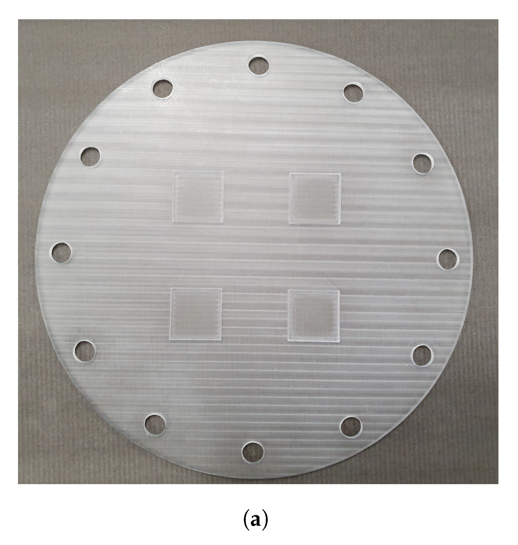
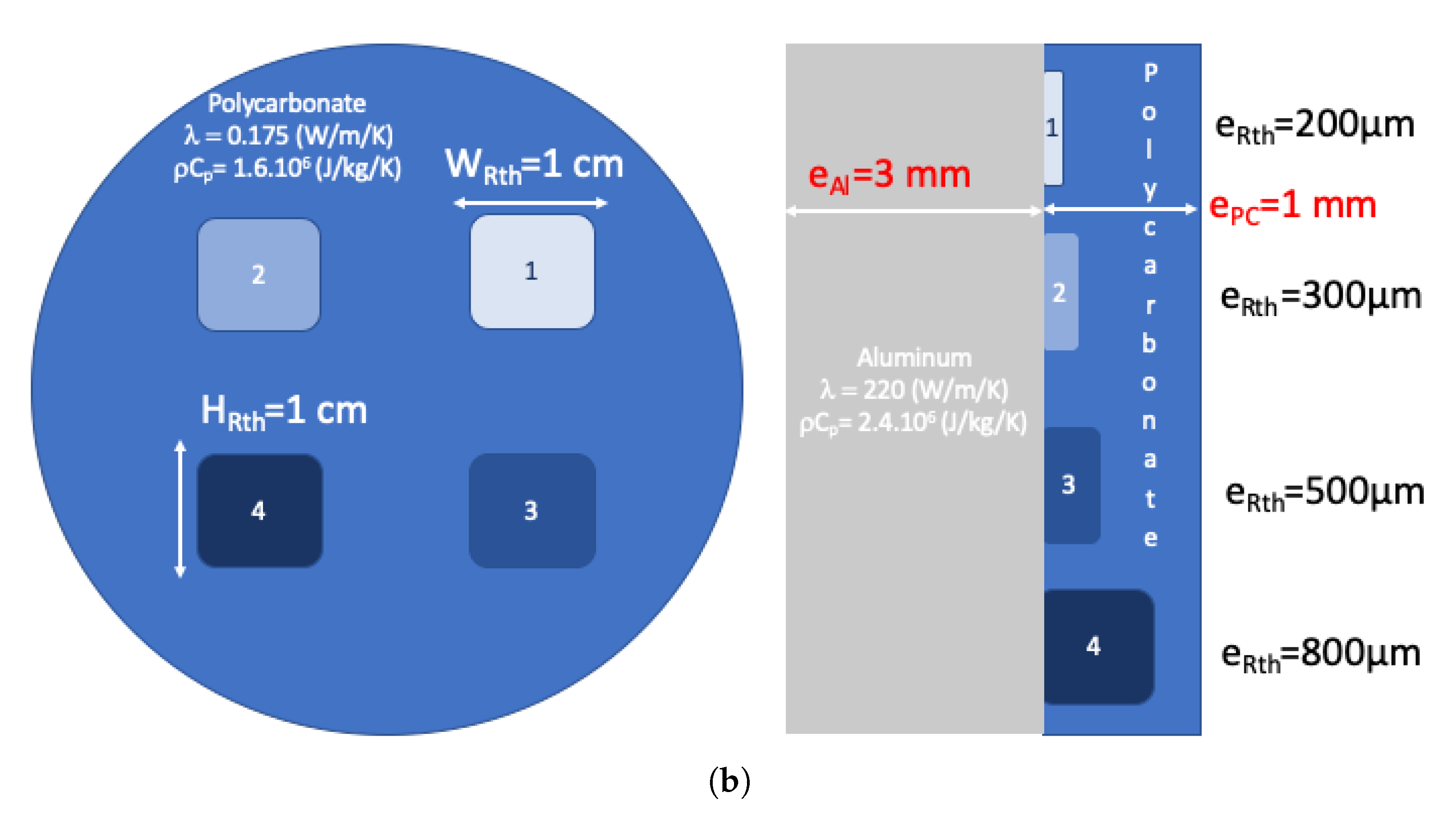
2. Experimental Setup and Materials
3. Methods
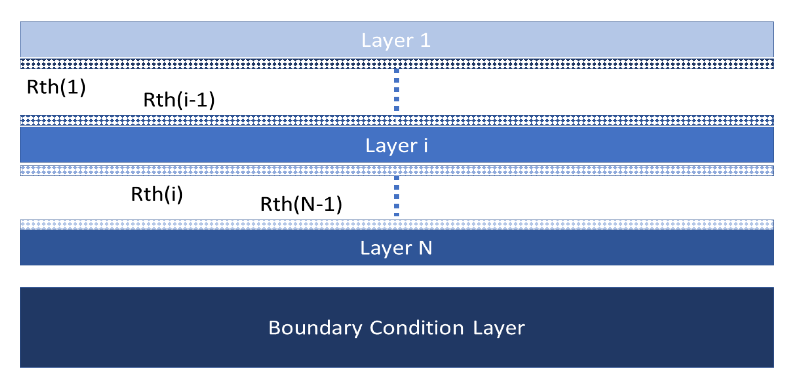
3.1. Direct Problem
3.2. Autoregressive Asymptotic Method
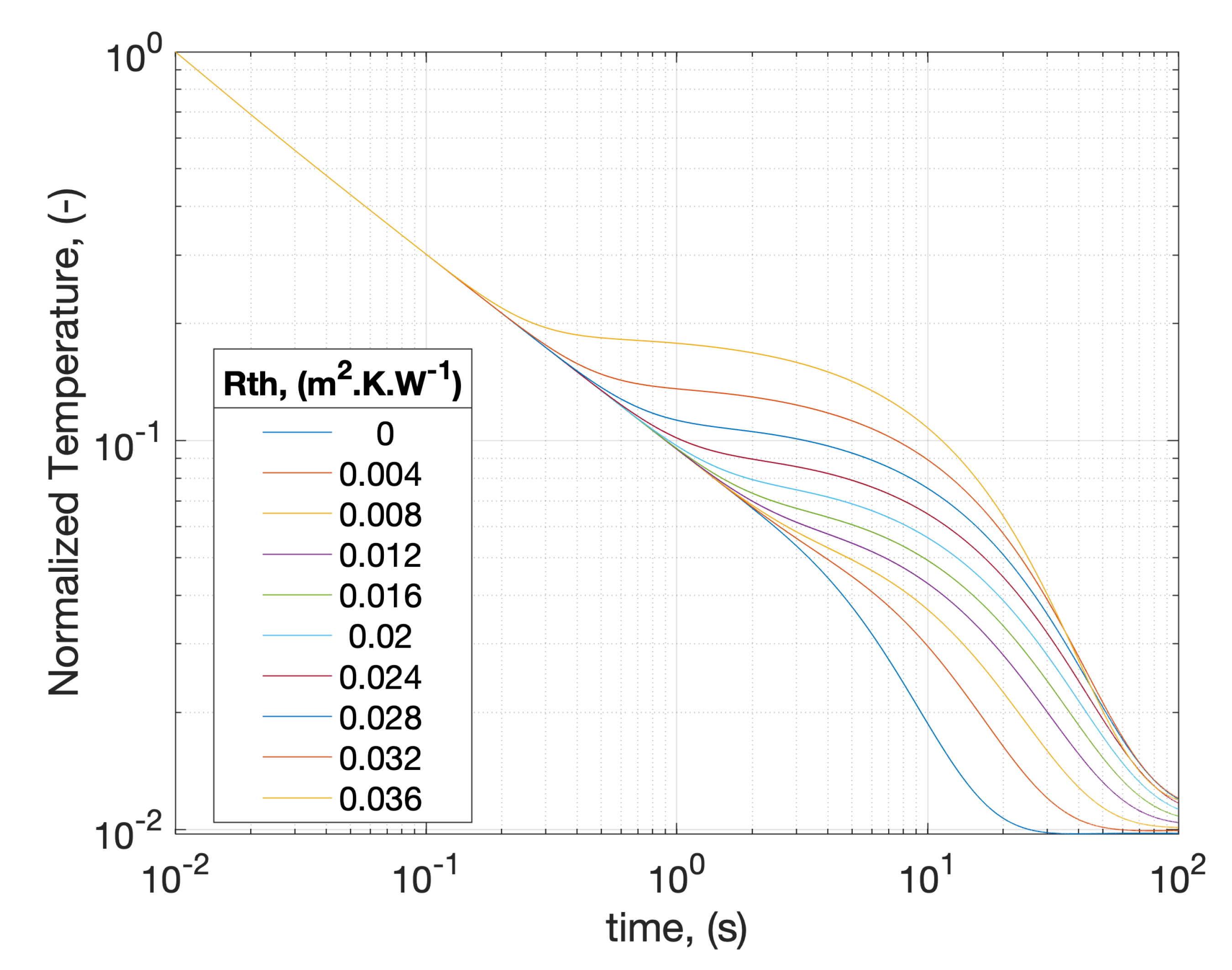
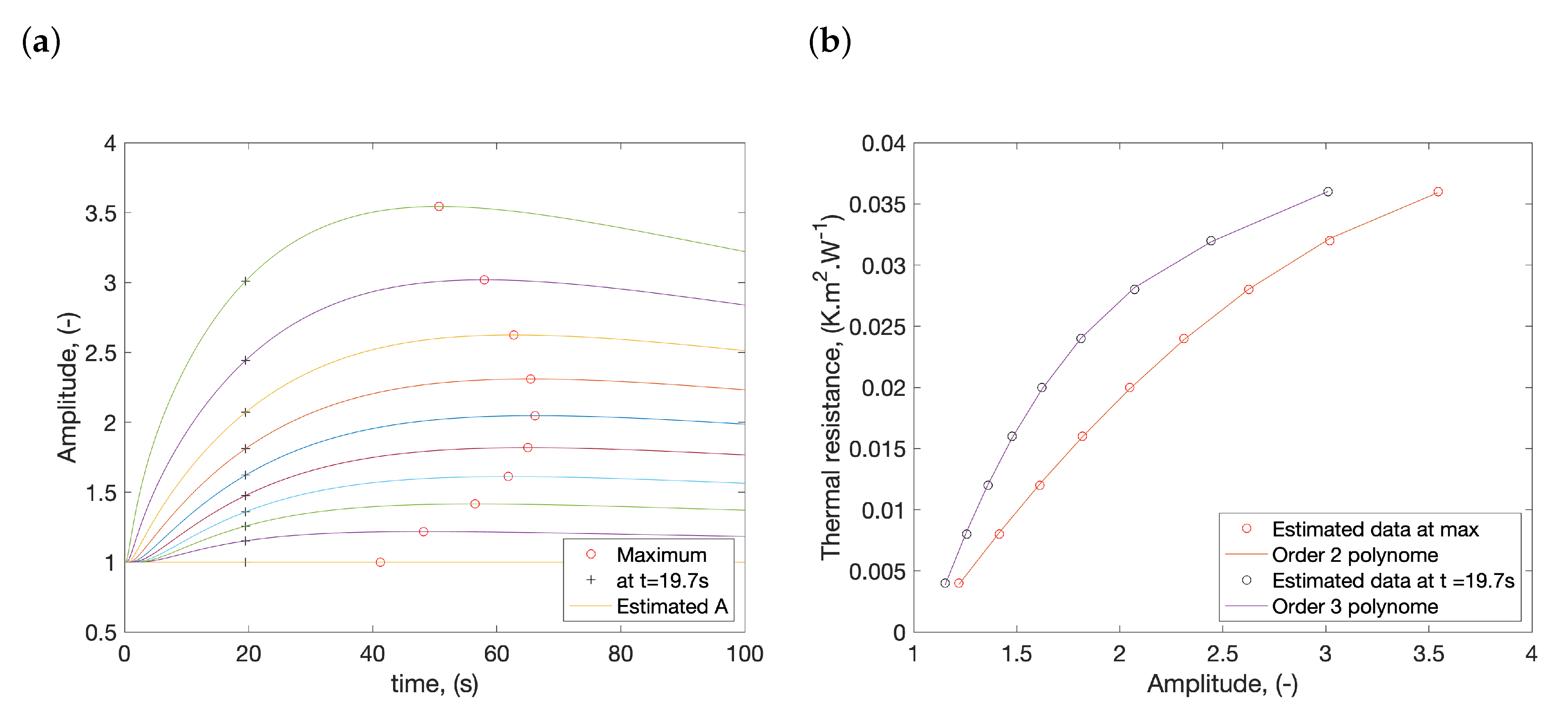
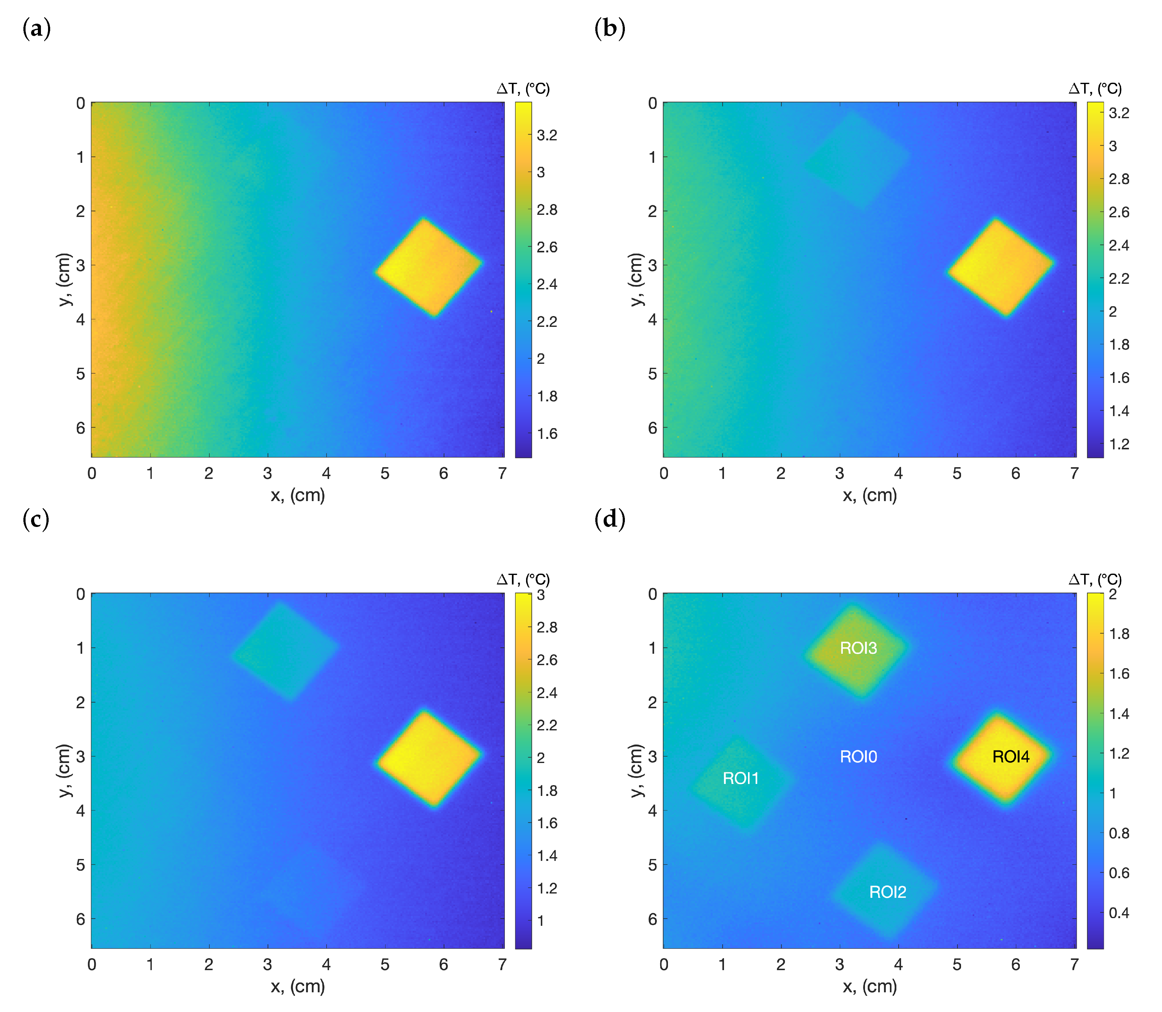
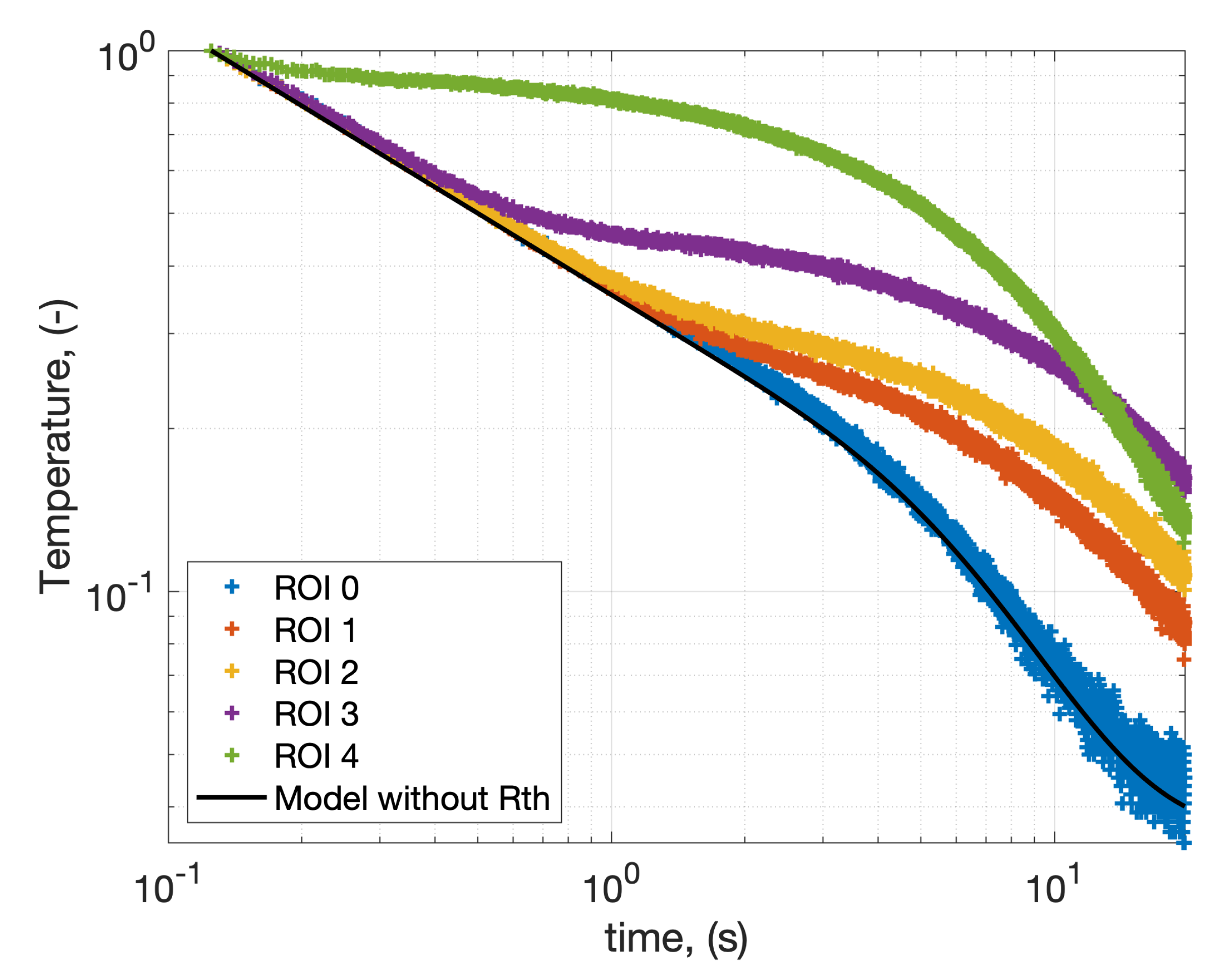
4. Results and Discussion
5. Conclusions
Author Contributions
Funding
Conflicts of Interest
References
- Cahill, D.G. Thermal conductivity measurement from 30 to 750 K: The 3ω method. Rev. Sci. Instrum. 1990, 61, 802–808. [Google Scholar] [CrossRef]
- Dilhaire, S.; Pernot, G.; Calbris, G.; Rampnoux, J.M.; Grauby, S. Heterodyne picosecond thermoreflectance applied to nanoscale thermal metrology. J. Appl. Phys. 2011, 110, 114314. [Google Scholar] [CrossRef]
- Baba, T.; Ishikawa, K.; Yagi, T.; Taketoshi, N. Measurements of thermophysical property of thin films by light pulse heating thermoreflectance methods. arXiv 2007, arXiv:0709.1845. [Google Scholar]
- Horny, N.; Chirtoc, M.; Fleming, A.; Hamaoui, G.; Ban, H. Kapitza thermal resistance studied by high-frequency photothermal radiometry. Appl. Phys. Lett. 2016, 109, 033103. [Google Scholar] [CrossRef]
- Depriester, M.; Hus, P.; Delenclos, S.; Sahraoui, A.H. New methodology for thermal parameter measurements in solids using photothermal radiometry. Rev. Sci. Instrum. 2005, 76, 074902. [Google Scholar] [CrossRef]
- Kusiak, A.; Battaglia, J.L.; Noe, P.; Sousa, V.; Fillot, F. Thermal conductivity of carbon doped GeTe thin films in amorphous and crystalline state measured by modulated photo thermal radiometry. J. Phys. Conf. Ser. 2016, 745, 032104. [Google Scholar] [CrossRef]
- Shepard, S.M. Flash thermography of aerospace composites. 2007. Available online: https://www.ndt.net/article/panndt2007/papers/132.pdf (accessed on 29 January 2020).
- Balageas, D.; Chapuis, B.; Deban, G.; Passilly, F. Improvement of the detection of defects by pulse thermography thanks to the TSR approach in the case of a smart composite repair patch. Quant. InfraRed Thermogr. J. 2010, 7, 167–187. [Google Scholar] [CrossRef]
- Karpen, W.; Wu, D.; Steegmuller, R.; Busse, G. Depth profiling of orientation in laminates with local lockin thermography. Proc. QIRT 1994, 94, 23–26. [Google Scholar]
- Oswald-Tranta, B.; Maier, A.; Schledjewski, R. Defect depth determination in a CFRP structure using TSR technique. In Proceedings of the 12th International Conference on Quantitative Infrared Thermography (QIRT 2014), Bordeaux, France, 7–11 July 2014. [Google Scholar]
- Roche, J.M.; Balageas, D. Imagerie quantitative TSR-RVB: De la détection de défauts au D-scan thermique. Available online: https://www.sft.asso.fr/Local/sft/dir/user-3775/documents/actes/Congres_2015/Communications/41753-fichier4.pdf (accessed on 29 January 2020).
- Ibarra-Castanedo, C.; Maldague, X. Pulsed phase thermography reviewed. Quant. Infrared Thermogr. J. 2004, 1, 47–70. [Google Scholar] [CrossRef]
- Shepard, S.M.; Lhota, J.R.; Rubadeux, B.A.; Wang, D.; Ahmed, T. Reconstruction and enhancement of active thermographic image sequences. Opt. Eng. 2003, 42, 1337–1343. [Google Scholar] [CrossRef]
- Müller, J.P.; Krankenhagen, R. Optimizing thermographic testing of thick GFRP plates by assessing the real energy absorbed within the material. Compos. Struct. 2019, 215, 60–68. [Google Scholar] [CrossRef]
- Maillet, D. Thermal Quadrupoles: Solving the Heat Equation Through Integral Transforms; John Wiley & Sons Inc.: Hoboken, NJ, USA, 2000. [Google Scholar]
- Bendada, A.; Erchiqui, F.; Lamontagne, M. Pulsed thermography in the evaluation of an aircraft composite using 3D thermal quadrupoles and mathematical perturbations. Inverse Probl. 2005, 21, 857. [Google Scholar] [CrossRef]
- Winfree, W.P.; Zalameda, J.N.; Howell, P.A.; Cramer, K.E. Simulation of thermographic responses of delaminations in composites with quadrupole method. Thermosense Ther. Infrared Appl. XXXVIII Int. Soc. Opt. Photonics 2016, 9861, 98610N. [Google Scholar]
- Bernegger, R.; Altenburg, S.J.; Roellig, M.; Maierhofer, C. Applicability of a 1D analytical model for pulse thermography of laterally heterogeneous semitransparent materials. Int. J. Thermophys. 2018, 39, 39. [Google Scholar] [CrossRef]
- Feuillet, V.; Ibos, L.; Fois, M.; Dumoulin, J.; Candau, Y. Defect detection and characterization in composite materials using square pulse thermography coupled with singular value decomposition analysis and thermal quadrupole modeling. NDT E Int. 2012, 51, 58–67. [Google Scholar] [CrossRef]
- Stewart, G.W. On the early history of the singular value decomposition. SIAM Rev. 1993, 35, 551–566. [Google Scholar] [CrossRef]
- Jordan, C. Sur la réduction des formes bilinéaires. Comptes Rendus De l’Académie Des Sciences 1874, 78, 614–617. [Google Scholar]
- Beltrami, E. Sulle funzioni bilineari. Giornale di Matematiche ad Uso degli Studenti Delle Universita 1873, 11, 98–106. [Google Scholar]
- Sylvester, J.J. Sur la reduction biorthogonale d’une forme lineo-linéaire a sa forme canonique. Comptes Rendus 1889, 108, 651–653. [Google Scholar]
- Dean, J.A. Lange’s Handbook of Chemistry; Mcgraw-Hill, Inc.: New York, NY, USA; London, UK, 1999. [Google Scholar]
- Touloukian, Y.S.; Powell, R.W.; Ho, C.Y.; Klemens, P.G. Thermophysical Properties of Matter-the tprc Data Series. Volume 1. Thermal Conductivity-Metallic Elements and Alloys; Thermophysical and Electronic Properties Information Analysis Center: Lafayette, IN, USA, 1970. [Google Scholar]
- Stehfest, H. Algorithm 368: Numerical inversion of Laplace transforms [D5]. Commun. ACM 1970, 13, 47–49. [Google Scholar] [CrossRef]
- Zheng, W.X. A least-squares based method for autoregressive signals in the presence of noise. IEEE Trans. Circuits Syst. II Analog Digit. Signal Process. 1999, 46, 81–85. [Google Scholar] [CrossRef]
- Moore, E.H. On the reciprocal of the general algebraic matrix. Bull. Am. Math. Soc. 1920, 26, 394–395. [Google Scholar]
- Penrose, R. A generalized inverse for matrices. In Mathematical Proceedings of the Cambridge Philosophical Society; Cambridge University Press: Cambridge, UK, 1955; Volume 51, pp. 406–413. [Google Scholar]


| Error *** | |||||
|---|---|---|---|---|---|
| (m) | (W.m.K) | (m.K.W) | (m.K.W) | (%) | |
| * ROI 1 | [200–250] ** | 0.025 | [0.008–0.01] | 0.0087 | 3.4 |
| * ROI 2 | [300–350] ** | 0.025 | [0.012–0.014] | 0.0126 | 3.1 |
| * ROI 3 | [500–550] ** | 0.025 | [0.02–0.022] | 0.0221 | 5.2 |
| * ROI 4 | [800–850] ** | 0.025 | [0.032–0.034] | 0.0328 | 0.85 |
© 2020 by the authors. Licensee MDPI, Basel, Switzerland. This article is an open access article distributed under the terms and conditions of the Creative Commons Attribution (CC BY) license (http://creativecommons.org/licenses/by/4.0/).
Share and Cite
Groz, M.-M.; Bensalem, M.; Sommier, A.; Abisset-Chavanne, E.; Chevalier, S.; Chulkov, A.; Battaglia, J.-L.; Batsale, J.-C.; Pradere, C. Estimation of Thermal Resistance Field in Layered Materials by Analytical Asymptotic Method. Appl. Sci. 2020, 10, 2351. https://doi.org/10.3390/app10072351
Groz M-M, Bensalem M, Sommier A, Abisset-Chavanne E, Chevalier S, Chulkov A, Battaglia J-L, Batsale J-C, Pradere C. Estimation of Thermal Resistance Field in Layered Materials by Analytical Asymptotic Method. Applied Sciences. 2020; 10(7):2351. https://doi.org/10.3390/app10072351
Chicago/Turabian StyleGroz, Marie-Marthe, Mohamed Bensalem, Alain Sommier, Emmanuelle Abisset-Chavanne, Stéphane Chevalier, Arsenii Chulkov, Jean-Luc Battaglia, Jean-Christophe Batsale, and Christophe Pradere. 2020. "Estimation of Thermal Resistance Field in Layered Materials by Analytical Asymptotic Method" Applied Sciences 10, no. 7: 2351. https://doi.org/10.3390/app10072351
APA StyleGroz, M.-M., Bensalem, M., Sommier, A., Abisset-Chavanne, E., Chevalier, S., Chulkov, A., Battaglia, J.-L., Batsale, J.-C., & Pradere, C. (2020). Estimation of Thermal Resistance Field in Layered Materials by Analytical Asymptotic Method. Applied Sciences, 10(7), 2351. https://doi.org/10.3390/app10072351