Stress Corrosion Cracking Threshold for Dissimilar Capacitive Discharge Welding Joint with Varied Surface Geometry

Abstract

Stress corrosion cracking (SCC) is known as a major factor that should be considered in the assessment of welding joint structure integrity. Despite the promising and wide application of dissimilar metal joints, the currently available SCC mitigation technique of dissimilar metal joints is not adequate. The challenge is to obtain a good joint while different melting points exist. This article reports a novel SCC mitigation method on a brass–steel dissimilar metal joint by modifying the geometry of the surface. It is evidenced that the sharpened steel (α1 specimen) significantly improves the SCC resilience of the joint. The evaluation of SEM/EDS photos reveals that the α1 geometry induces a smaller pore area around brass–steel micro-joint interfaces which in turn produces stronger joints.

1. Introduction

Stress corrosion cracking (SCC) originating from a welding joint is the predominant factor of the steel pipeline failure in a harsh environment. The SCC in many occasions causes the collapse of high-pressure gas transmission pipes that leads to significant economic loss, as well as environmental and health risks [1,2]. Wan et al. evaluated the welded joints of X65 steel exposed in the shallow deep sea [3]. It is found that the high hydrostatic pressure, low hydrogen, and temperature trigger localized corrosion induced SCC [4,5]. Various efforts have been conducted to understand and mitigate the SCC in stainless steels and their welding joints; however, these studies mostly focus on the welding joints of similar metals while the real challenge in dissimilar metal welds is still overlooked [6,7,8]. Dissimilar welding promotes a strenuous task due to the melting point difference [9]. From the SCC’s point of view, the resulted dissimilar metal joint is more susceptible to the SCC. Recently, it has been suggested that post-welding heat treatment could improve the resilience of dissimilar metal welding joints to the SCC load [10].

There are several methods that have been developed to carry out dissimilar welding joints. To “joint” plates, the explosive welding (EXW) may be the most effective process to clad certain metals onto the surface of another metal. A literature study of EXW application and research is provided by Findik [11]. TA1 (Titanium Alloy grade 1) with high corrosion resistance has been clad successfully to X65 high strength steel [12], while other welding methods produce brittle intermetallic Fe-Ti compounds which usually initiates failure. Ti6Al4V was clad on Inconel 25 [13]. When 600 °C annealing was applied, the ductility was increased, but no other mechanical properties were improved. A5086 aluminum alloy was clad on American Society for Testing and Materials (ASTM) A516 low carbon steel with pure aluminum as intermediate layer using EXW [14]. Inspection using digital image showed that the higher strain takes place at the aluminum side. Infrared thermography was used to predict the fatigue life of the Bimetal and the result from the experiment verified the prediction. A non-linear finite element analysis was able to emulate the EXW well [15], which may be used as intellectual control of the EXW process in the future. Recently, solid state welding has been proposed to join dissimilar metal or metals with low weld ability in terms of “conventional” fusion welding. A review study on the application of solid state welding to join dissimilar metals has been published [16]. The effect of parameters on the resulted strength of the joint has also been studied, such as the effect of pressure force [17] and the length of the pin [18].

Capacitive discharge welding (CDW), which may be also called Capacitor Discharge Welding, is a form of resistance welding where the energy is drawn from a stored energy in a capacitor instead of directly from the grid. Unlike EXW, which is typically applied on quite large-sized plates, CDW can be applied on small-sized metal bars. Using the stored energy, the time of the welding process is short and concentrated (one tenth of typical resistance welding [19]). Using a high speed camera [20], it can be concluded that the CDW process is one-dimensional due to fast arc spread upon ignition [21]. A wide application of the CDW on the automotive area in North America is accelerated due to the need of dissimilar welding to provide lightweight cars. In a lightweight car, exhibiting welding of hot-stamped boron steels and aluminum–silicon coated steels is needed, which on many occasions is unevenly clad. CDW has also been used to join pipes and/or tubular parts [22]. To obtain good joints of the tubular parts, grooving or indentation (surface preparation) is needed.

Based on the above literature study, this research evaluates the SCC behavior of a dissimilar joint which is produced by the CDW process. In this article, we offer a facile method in improving the resiliency of dissimilar metal welding joints toward the SCC formation by modifying the interface geometry of the joints. We studied steel and brass joints in connection with their potential combination of an adequate strength of steel and disinfectant-oligodynamic characteristics of brass that may be useful for broad applications [23]. These two combined properties (adequate strength and disinfectant) may utilize for medical tools and foods sets. The main resilience of the joints was represented by their SCC threshold. There are two types of SCC test: Slow Strain Rate Tension (SSRT) and Constant Load Test (CLT). This paper applied the CLT due to its simplicity, although a longer time is needed. Other supported data, such as macrophotos of fracture surfaces, microstructures, Scanning Electron Microscope (SEM), Energy Dispersive X-Ray Spectroscopy (EDS), and ultimate tensile strength are also discussed to obtain complete description.

2. Materials and Methods

Two bars of different metal were joined using the CDW process to form Dissimilar Metal Welds (DMWs). The metals were steel and brass. Their composition can be seen in

Table 1. Materials Composition.

Materials	Composition (weight %)
Low Carbon Steel	Fe	C	Al	S	Cr	Si	Ni	P	Cu
	Bal	0.148	0.001	0.02	0.046	0.0015	0.092	0.008	0.103
	Mn	W
	0.555	0.04
Brass	Ag	Al	Bi	Cd	Co	Cr	Cu	Fe	Mg	Mn
	<0.01	1.55	0.006	<0.01	<0.01	0.006	57.01	0.56	0.03	0.08
	Mo	Ni	Pb	Sb	Sn	V	Zn
	<0.01	0.35	2.22	0.04	0.98	<0.01	36.51

and their properties are listed in

Table 2. Properties.

Materials	PROPERTIES
	Melting point (°C)	UTS N/mm2	Hardness BHN	Density (g/cm3)
LC Steel	1450	440	120	7.87
Brass	899	345	100	8.40

. Both materials are solid rod with a diameter of 1.6 mm. The length of the bar which will be welded is 40 mm.

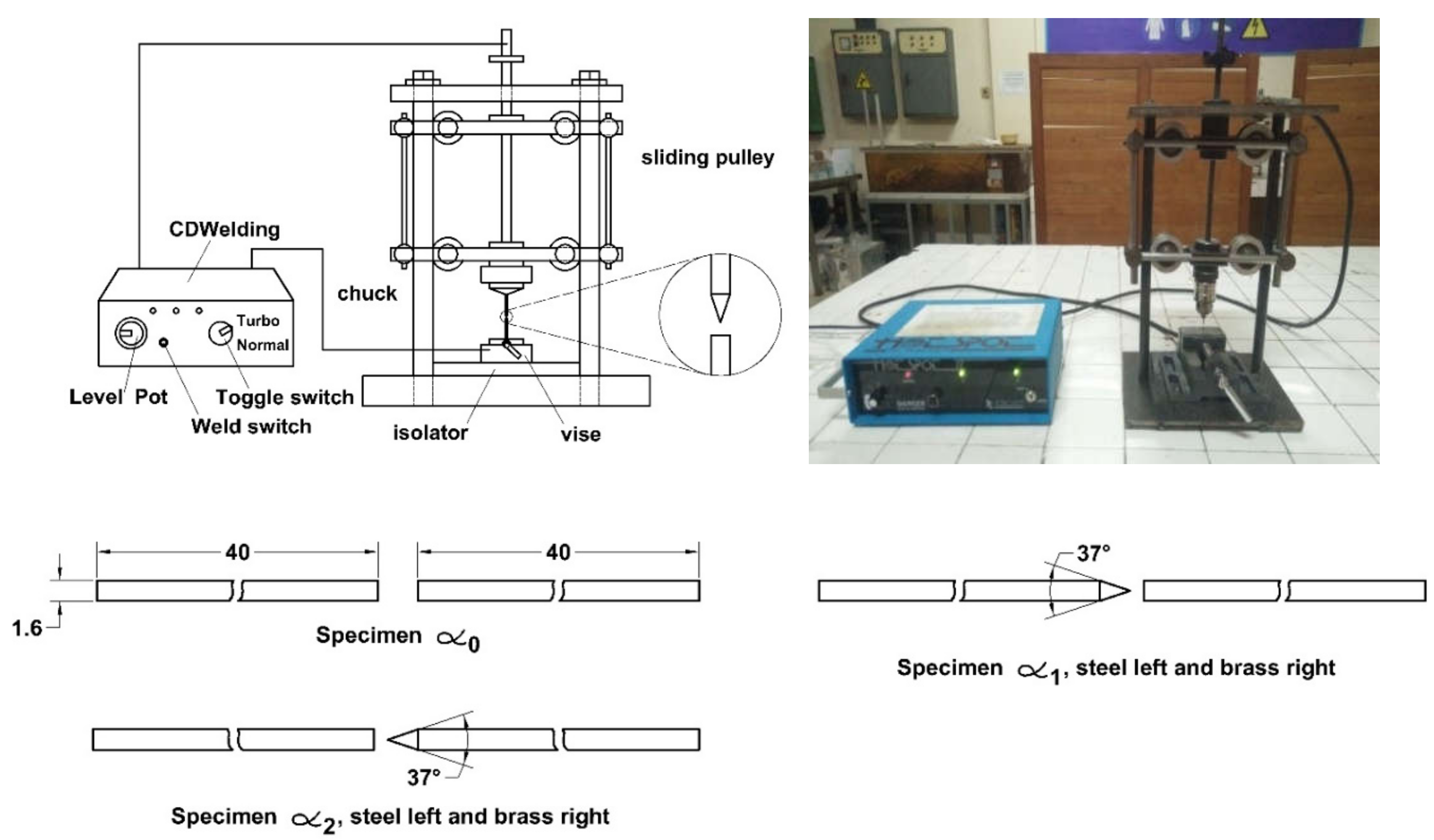
The CDW process was carried out using a special jig which was designed for this experiment and can be seen in Figure 1. Figure 1 shows a sketch and a photo of the CD Welder. With the special jig, welding parameters can be maintained in equal values or conditions. The inputted power, which in turn determines the heat input, was 120 Joule and the voltage was 75 Volt DC. The normal pressure is assumed equable by setting the load and tip distance before the drop, which were 4 kg and 5 mm, respectively.

The independent variable of this research is a different surface preparation, which is described in the lower part of Figure 1 and called α0, α1, and α2. In the figure, for the steel that is always on the left side, or also termed specimen α0, both surfaces are flat, while for specimens α1 and α2, the steel and brass are sharpened, respectively. It should be noted that, for the sharpened surface at two tips the good joint was hard to be obtained and always produced misaligned components. Thus, there is no specimen with a sharpened tip for both metals. For all surface combinations, the steel, which has better weldability, was always gripped at upper chuck to obtain better results. Using all the described methods, welding parameters were considered to be constant, and the only altered parameter is the surface preparation, which is the only independent variable in this article.

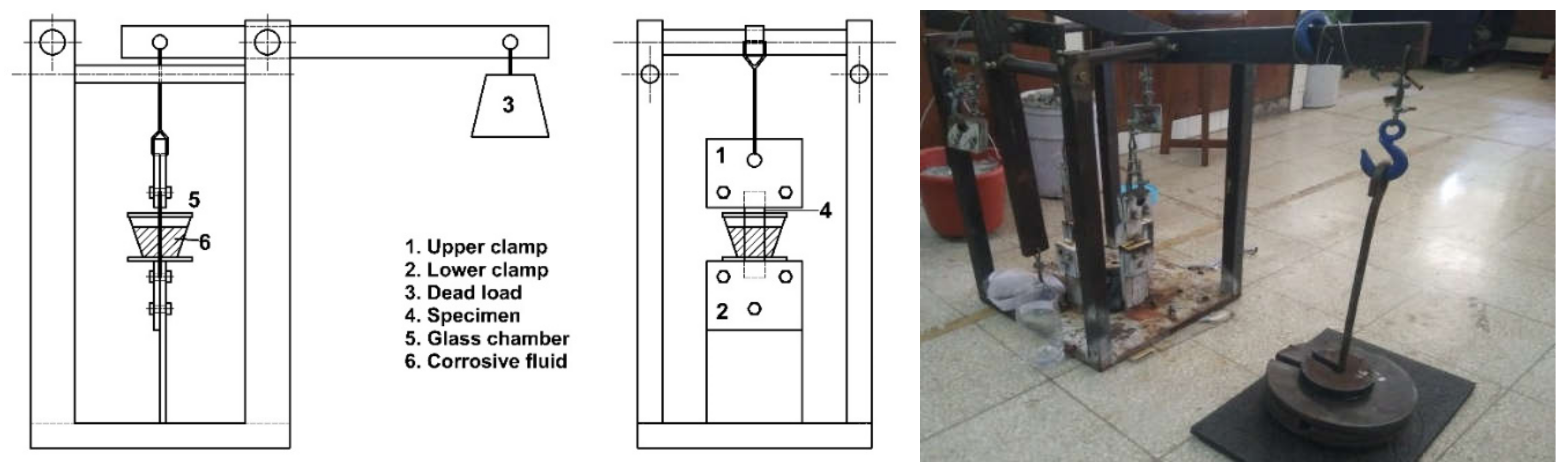
After the joints were obtained, the next step was the SCC corrosion test, which is the dependent variable of this article. The focus for the dependent variable is the stress corrosion threshold, which describes the maximum stress, which is defined as the maximum allowed exerted stress where the SCC is assumed to not occur. Figure 2 shows the installation of the SCC, which was designated for this research. Figure 2 shows a sketch and a photo of the SCC apparatus. The dead load is attached at the end of the loading arm (right arm) and the applied load at the upper clamp can be counted by considering the length of each arm. The exerted tensile stress can be calculated by dividing the load by the original area of the base metal (πD²/4). The specimens, especially the interface, were dipped in the 1 Molar HNO3 solution. To obtain the SCC threshold, the load must be varied, and for each load the time to fail was recorded.

The morphology of welded interfaces was analyzed using Hitachi SEM/EDS type FLEXSEM 100. The backscattered electron (BSE) was used to characterize the high magnification of cracks/voids of the welding joint. The composition mapping of the joint interface was analyzed using Energy Dispersive X-Ray Spectrometry (EDS).

3. Results and Discussions

As has been explained in Section 2, the dependent variable is the time to failure for the varied load. The load at the end of the arm (see Figure 2) was varied at 8, 10, 12, 14, 16, 18, 20, 22, and 24 kg, which can be converted into the tensile load for the specimen as follows: 115, 144, 173, 201, 230, 259, 288, 316, and 345 MPa, respectively. For each variation of load, three data of time to failure were recorded. In practice, the data were recorded in hours, minutes, and seconds, but for easy data processing they are tabulated in minutes. As an example, two hours, ten minutes, and thirty seconds are tabulated as 120 minutes, 10 minutes, and 0.5 minutes, which equals 130.5 minutes. The complete recorded data are presented in

Table 3. SCC test results.

Load (kg)	Stress (MPa)	α0		α1		α2
		Time to Fail (minute)	Mean (minute)	Time to Fail (minute)	Mean (minute)	Time to Fail (minute)	Mean (minute)
8	115	180.75	184.02	-	N/A	-	N/A
		183.67		-		-
		187.63		-		-
10	144	37.17	36.41	-	N/A	-	N/A
		36.67		-		-
		35.38		-		-
12	173	17.72	17.26	-	N/A	179.50	180.35
		17.22		-		180.48
		16.83		-		181.07
14	201	7.85	7.47	-	N/A	31.33	31.28
		7.37		-		30.68
		7.18		-		31.83
16	230	2.57	2.25	186.28	185.66	7.95	8.10
		1.97		185.38		7.58
		2.22		185.32		8.80
18	259	0.00	0.00	45.00	42.19	2.23	2.44
		0.00		41.22		2.67
		0.00		40.37		2.42
20	288	0.00	0.00	13.93	14.60	0.00	0.00
		0.00		14.78		0.00
		0.00		15.08		0.00
22	316	0.00	0.00	5.52	5.31	0.00	0.00
		0.00		5.15		0.00
		0.00		5.27		0.00
24	345	0.00	0.00	0.00	0,00	0.00	0.00
		0.00		0.00		0.00
		0.00		0.00		0.00

that shows the time to failure for varied surface preparation and load when the joint is exposed to the corrosive environment. When a load of 24 kg (345 MPa tensile stress) was applied, the welded joints failed immediately, since the load exceeded the ultimate strength of all joints. The α1 specimen revived around 5 minutes when 22 kg (316 MPa tensile stress) was applied whilst failure took place directly for two other specimens: α0 and α2. The 22 kg load roughly proved that the α1 specimen was the strongest joint by means of SCC threshold. The time to fail for the α1 specimen was obtained from three of α1 specimens to provide statistical acceptable data. The 316 MPa was considered to exceed the ultimate tensile strength of α0 and α2 specimens. When 250 MPa was applied, only the α0 specimen broke instantaneously while the others stood for a certain time, which more or less proved that the modified surface preparation improved the strength of the indigenously flat interfaces welded joint.

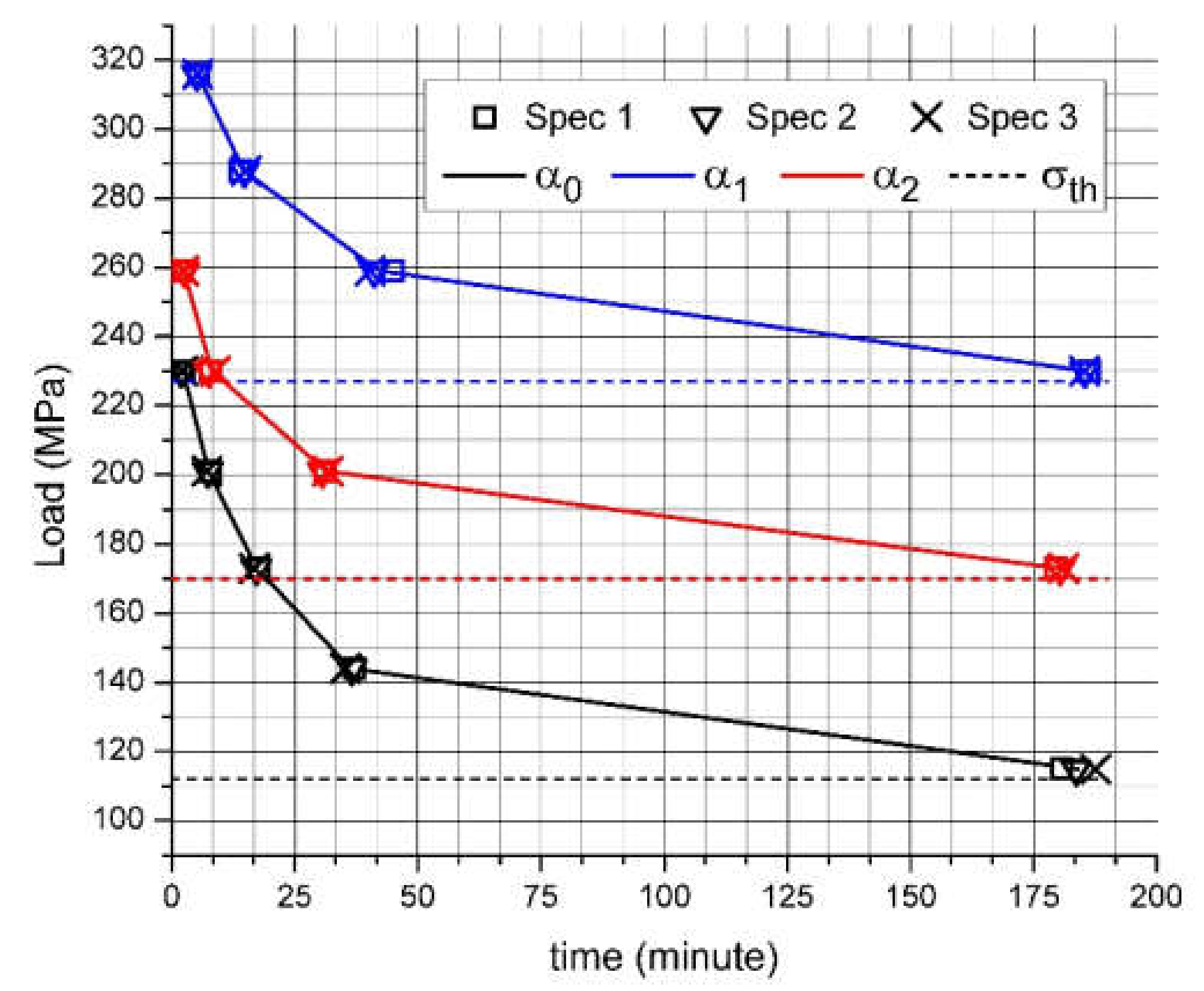
Table 3 represents in graph form what is depicted in Figure 3. For each treatment (certain load and surface preparation), data from three specimens were recorded. The first specimen, namely Spec 1, is represented using square symbols whilst the second and the third specimens, i.e., Spec 2 and Spec 3, are plotted using reversed triangles and cross symbols, respectively. Specimens without surface preparation, i.e., α0 specimen, are drawn in red color, whilst specimens with sharpened steel and sharpened brass are shown in red and blue colors, respectively. 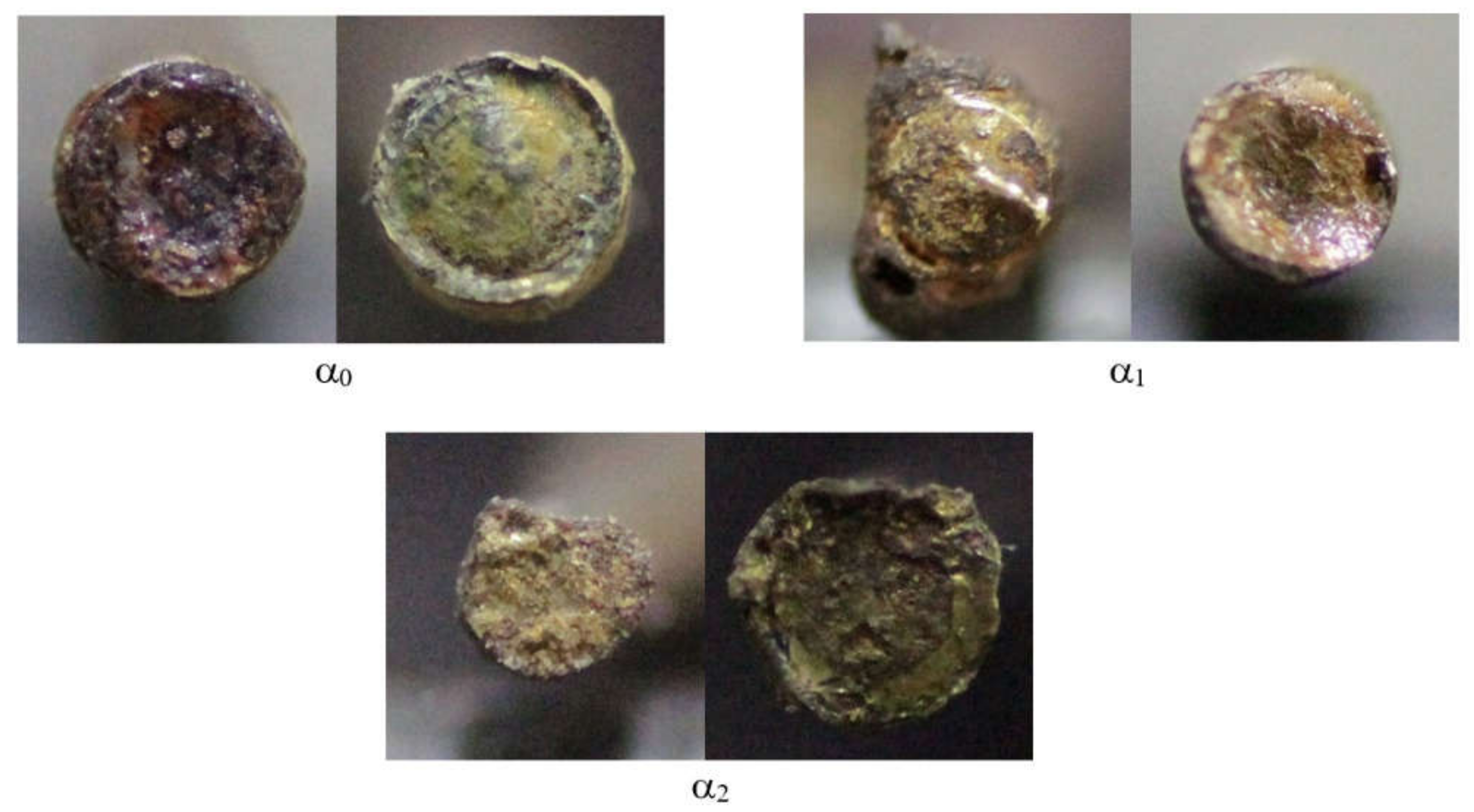From Figure 3, it can be concluded that the modification of the surface geometry does increase the resilience of the CDW joints to the SCC, which both the α1 and α2 specimens exhibited with a better performance on the SCC load compared to the flat interfaces of α0. For the α0 specimen, the stress corrosion cracking threshold can be assumed with 112 MPa, and for the α1 and α2 specimens with 227 MPa and 170 MPa, respectively, which shows the modified interfaces improve the SCC resilience significantly. The reason of the better performance, which is shown by the α2 and α1 specimens, can be obtained by evaluating the fracture surface of the welding joint. The macrograph of the fracture surfaces of α0, α1, and α2 is shown in Figure 4.

From Figure 4 it can be seen that the α1 specimens produce better coalescence, which is shown by the fracture on the steel and brass bars. By nature, the steel shows a black color in Figure 4 whilst the brass tends to be yellow. On the fracture surface of the α1 specimen, quite a lot of yellow dimples can be observed on the steel bar (left side), which represent the brass. Conversely, black dimples can be found on the brass bar (right side) for the steel. This appearance proves that by sharpening the steel bar, better smelting was obtained, which in turn improves the performance of the joint under a SCC load. The same trend is also found in the α2 specimen, but in a smaller number, while for the α0 specimen, no such dimples were found on the fracture surface, which shows the bad coalescence of the interface. Another confirmation can also be taken from the flash which develops in the joint. In the α1 specimen, a lot of flash is found in the fracture photo, especially in the steel bar. A small number of flashes can be found in the α2 specimen, especially on the brass side. It should be noted that it seems the flash was built at the sharpening side. The last and the least number of flashes can be found at the flat interface of specimen α0. The larger flash showed better melting. Evaluating the flashes confirms the obtained stress corrosion cracking threshold of Figure 3.

Our recent study suggests that the welding joint is more susceptible to the SCC when the welded materials have more residual stresses and voids. The void acts as crack initiator and may grow and form cracks [6,24]. Considering the embedded residual stresses and cracks, which easily occur in the welded joint: once it is exposed to the corrosive surroundings, all three ingredients of SCC are provided and the SCC failure exists in the welded joints.

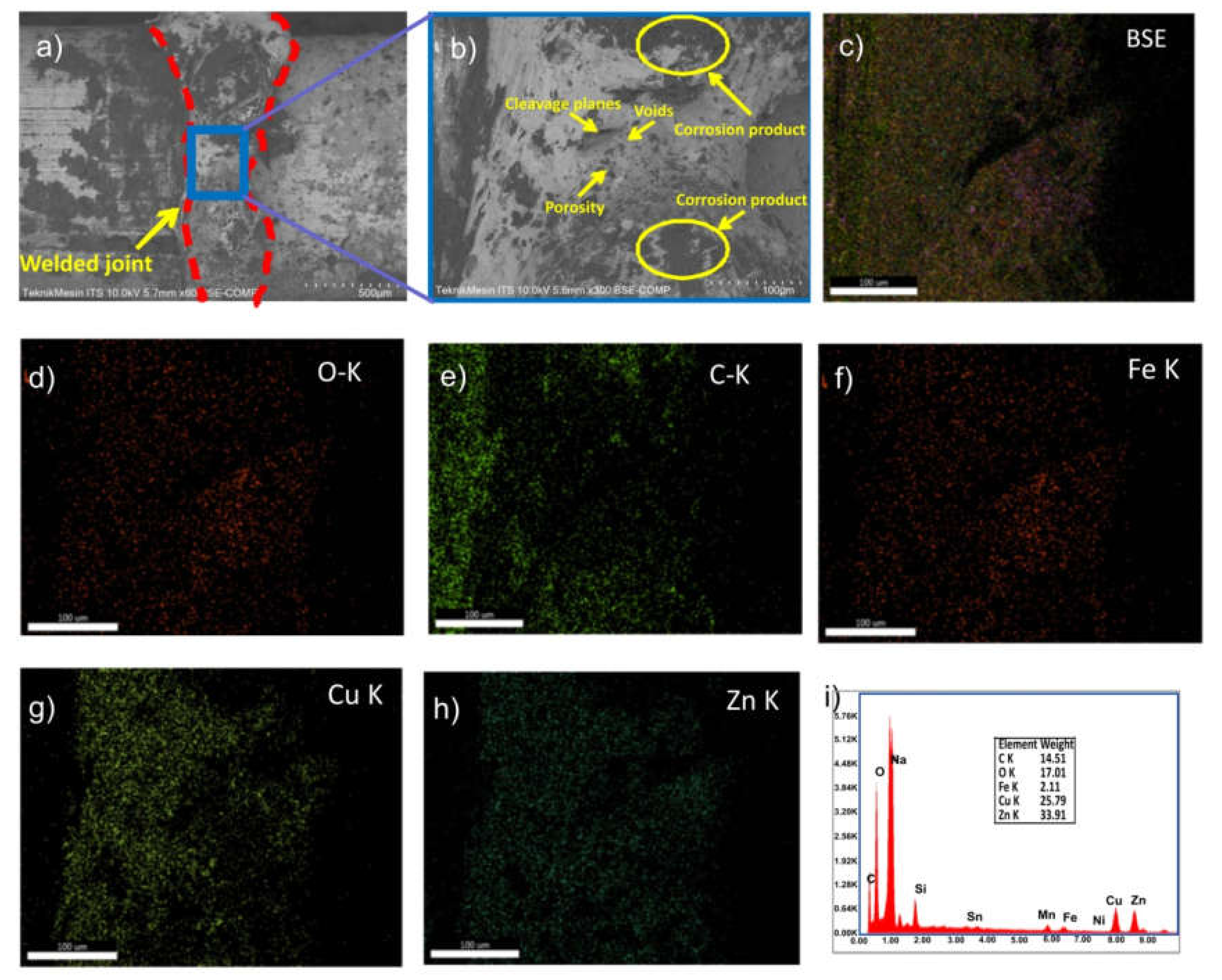
The SEM/EDS evaluation of the welded interface of the α0 specimen is shown in Figure 5. Figure 5a shows the interface with a 50x magnification. Figure 5a also shows the position where the EDS was applied. The position where SEM/EDS was exhibited in the joint between mild steel and brass is shown in Figure 5b. It can be seen that there are porosity and fibrous networks, which initiate fracture at the welded joint. The fibrous network indicates the ductile fracture [25]. The local pit corrosion is spread over the interface. The existence of the O element indicates the oxidation of the welded joint when exposed to the HNO₃ solution. The increasing C is able to promote local pitting corrosion. Figure 5d–g shows a mapping of C, O, Fe, Cu, and Zn elements. It should be noted that Fe-C is the major element of mild steels whilst Cu and Zn are the dominant elements of brass. In the interface, the elements of Cu and Zn increase, which indicates that the brass deliquesce easier than steel. This is plausible since the melting point of brass is lower.

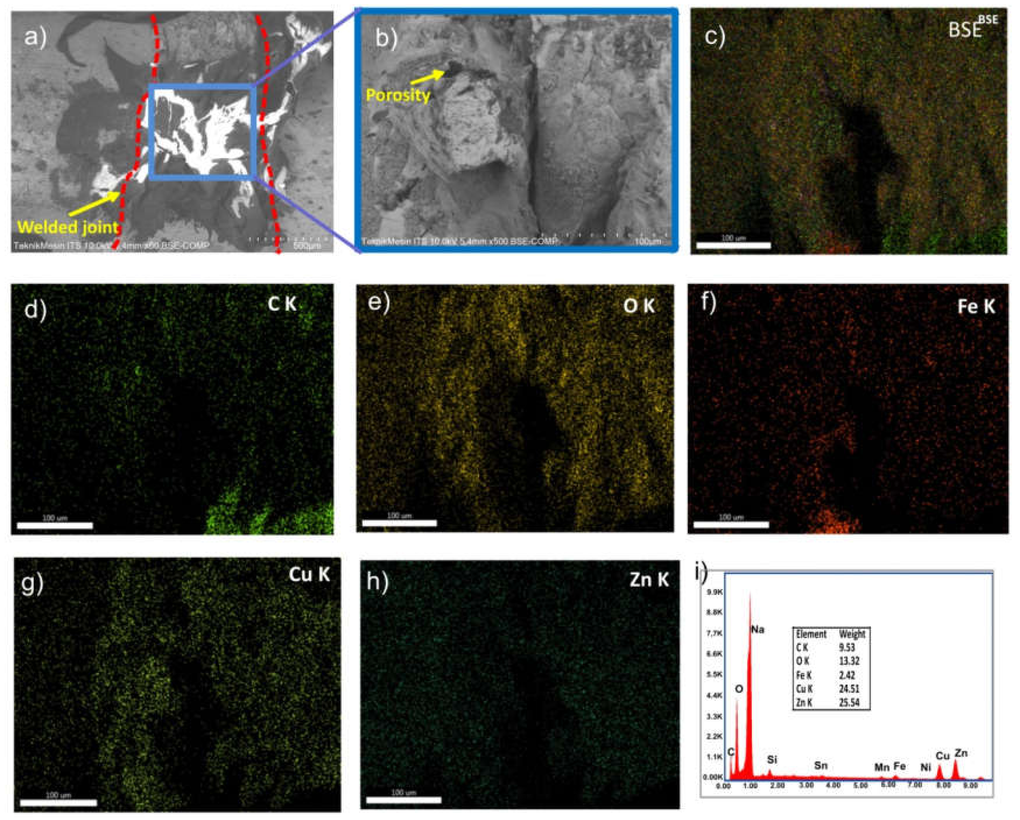
Figure 6 shows the SEM/EDS photos of α1 specimens. Compared to Figure 5, it can be seen that less void and corrosion products are found. As in Figure 5, Cu and Zn dominate more than Fe, although both elements are less compared to the α0 specimen. The O element decreases, which indicates that less oxidation took place, which in turn increases the strength of α1.

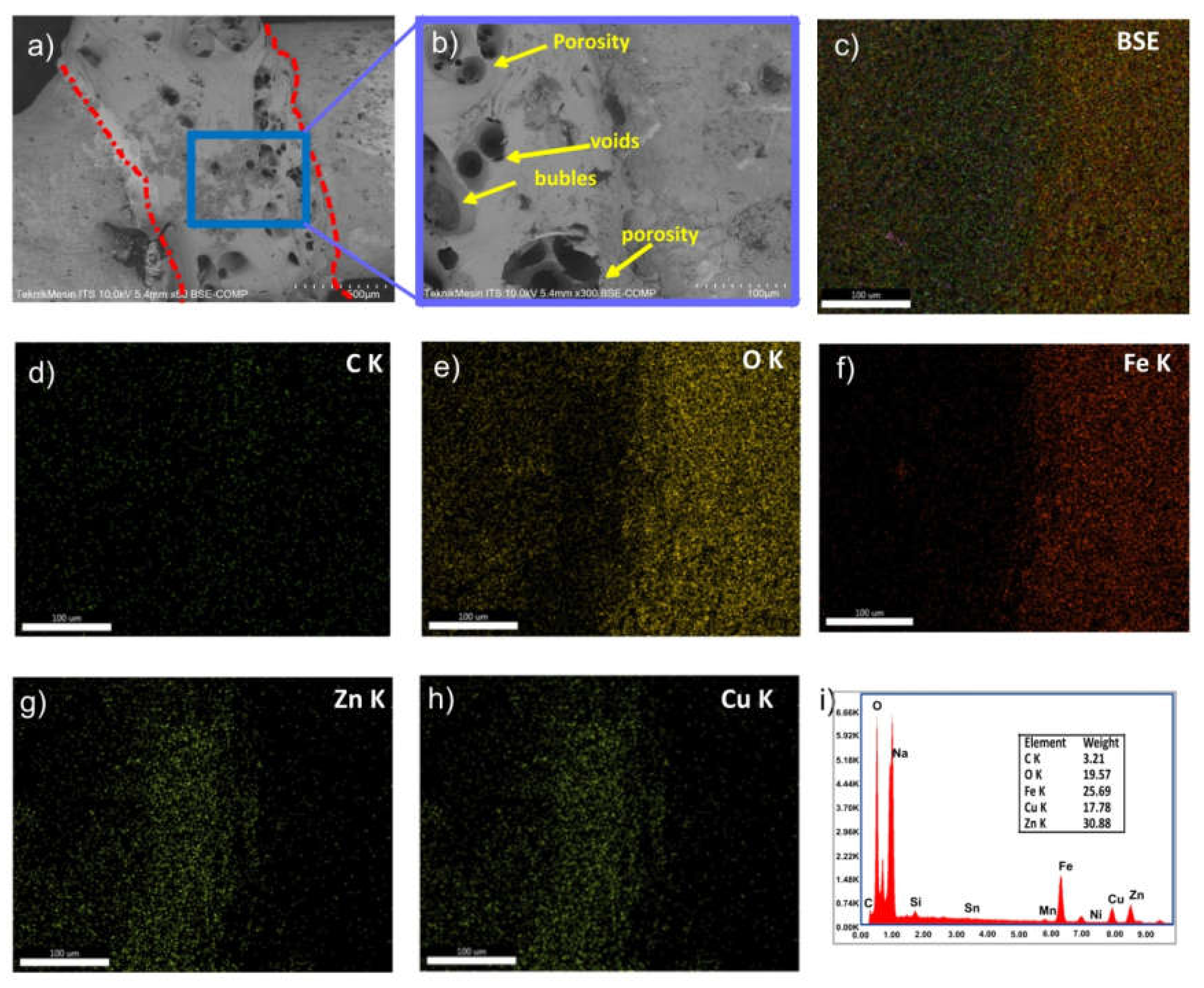
SEM/EDS photos for the interface of the α2 specimen are shown in Figure 7. There are many porosity, voids, and bubbles. The high O element provides the local corrosion. Compared to α0, only bubbles exist in α2 and no pits are available. The bubbles certainly cause the joint to become porous and fragile.

To evaluate the porosity, the analysis of the surface photo is shown in Figure 8. In the α2 specimen, the tapered surface of brass makes it easier to melt and coalesce to the steel surface. By nature, the steel (Fe) easily reacts with the oxygen in the HNO₃ [26]. These two phenomena can trap the air in the interface. The higher Fe content in α2 specimen increases the possibilities of the air trapped in the joint. The lesser amount of porosities, voids, and bubbles in α1 compared to α2 specimens confirms the stronger joint of the tapered steel configuration (α1).

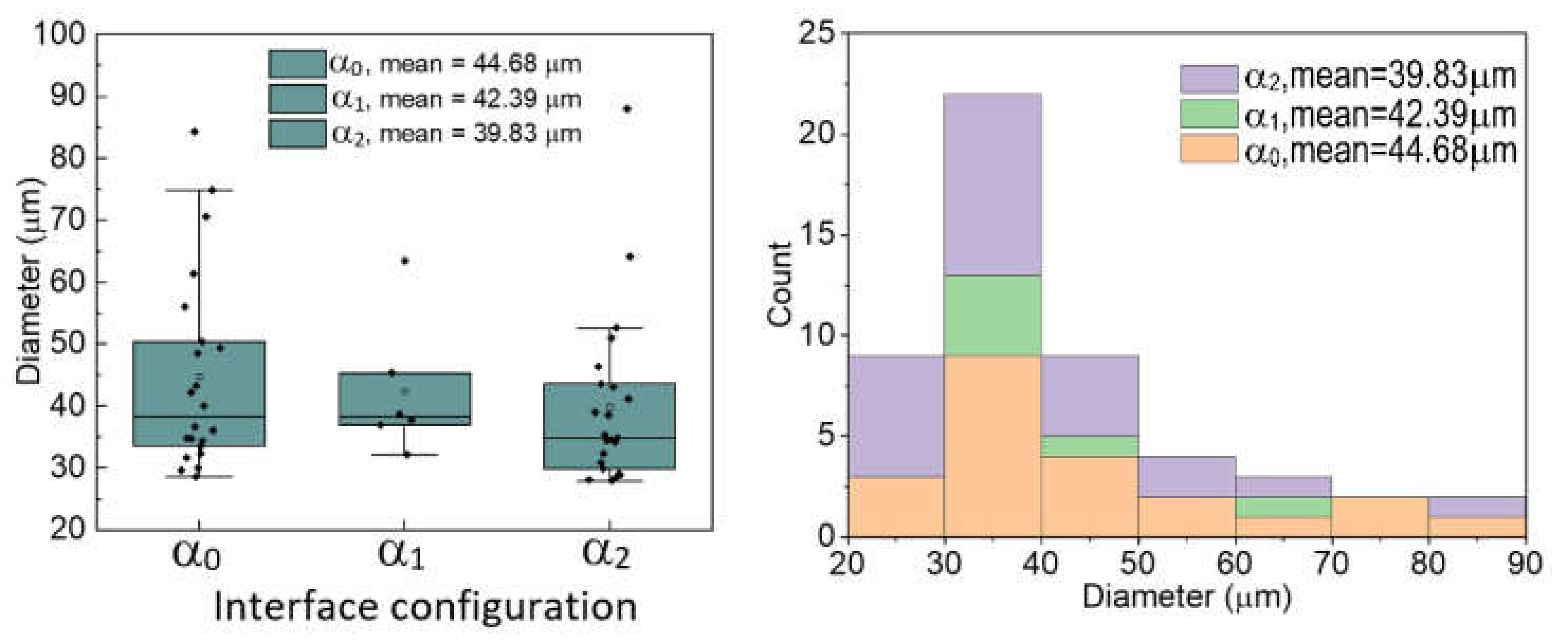
The quantitative analysis of pores was carried out using Phenom Phorometric analysis which is attached as Supplementary Materials of this paper. The mean pore size of α0, α1, and α2 are 44.7 μm, 42.5 μm, and 39.8 μm, respectively. Many pores are found in the α2 specimen with the lowest diameter. The distribution can be seen in Figure 8. α0 exhibits 22 pores with an average pore area ratio of 9.09%, calculated for one image. Observing the α1 image, six pores with an average pore area ratio of 1.13% are found, calculated for one image; whilst 23 pores are found for α2 with an average pore ratio of 4.96%, calculated for one image. The higher pore area ratio indicates the weaker welding joint. The α0 specimen shows a big amount of porosity since no melting existed at the steel and brass interfaces. Gaps on the interfaces take place in pore forms. The existence of a gap indicates that there is trapped air that forms visible pores. Big porosity on the welded joint enables a long crack in form of a line, and the product of corrosion spread over the joint surface. Based on microphotograph only, the strongest joint may be provided by the α1 specimen since this joint has the smallest porosity ratio. This confirms the macrophotograph of Figure 4 and the SEM/EDS analysis of Figure 8. On the α2 specimen, more porosity can be seen compared to α1. Although melting takes place at the interface of steel and brass, higher porosity and impurity decrease the strength of the joint. The decreased diameter and lower melting point of brass produces more brass deposit on α2 than on α1. In short, it can be said that the result of the SEM/EDS and porosity analysis supports the results of the SCC test: the strongest joint is obtained from the α1 configuration followed by α2 and α0, sequentially.

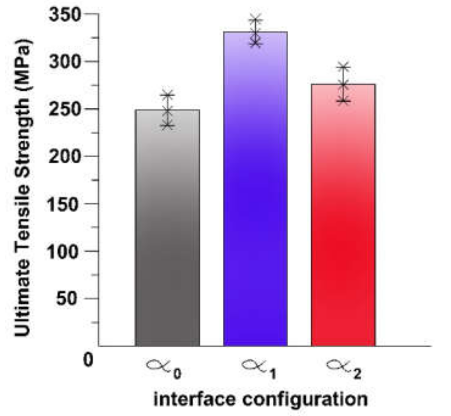
To prove the better coalescent of α1, we roughly obtained the tensile strength of the joint. Using the SCC apparatus (Figure 2), the ultimate tensile strength of the joint can be approached. The dead load at the end lever was increased gradually until the joint was broken. The ultimate tensile strengths were then presented in Figure 9. Three specimens were tested for each configuration. By this simple approach, the strongest joint was α1 followed by α2 and α0, consecutively, which supports all previous discussions.

4. Conclusions

The modified interface does improve the SCC resilience of a CDW dissimilar metal joint. The improvement is a result of better coalescent between interfaces, which is confirmed by evaluating the macrograph of the fracture surfaces and the existence of a flash. The microstructure observation also supports the SCC results. Without an interface modification (α0 specimen), the SCC threshold is 112 MPa. Sharpening the brass (α2 specimen) produces a 170 MPa SCC threshold whilst for the sharpened steel (α1 specimen) interface the strongest threshold of 227 MPa SCC is provided. The microstructure also follows this trend. Without modifying the interface, there is no melting that exists between steel and brass as shown by the micrograph of the α0 specimen. The α0 specimen had the biggest number of an average pore area due to the absence of melting. Regarding the portion pore area, the α1 specimen showed the smallest number, which shows good coalescent of steel and brass and in turn provides the strongest joint.