Multifocus Image Fusion Using a Sparse and Low-Rank Matrix Decomposition for Aviator’s Night Vision Goggle

Abstract

This study proposed the concept of sparse and low-rank matrix decomposition to address the need for aviator’s night vision goggles (NVG) automated inspection processes when inspecting equipment availability. First, the automation requirements include machinery and motor-driven focus knob of NVGs and image capture using cameras to achieve autofocus. Traditionally, passive autofocus involves first computing of sharpness of each frame and then use of a search algorithm to quickly find the sharpest focus. In this study, the concept of sparse and low-rank matrix decomposition was adopted to achieve autofocus calculation and image fusion. Image fusion can solve the multifocus problem caused by mechanism errors. Experimental results showed that the sharpest image frame and its nearby frame can be image-fused to resolve minor errors possibly arising from the image-capture mechanism. In this study, seven samples and 12 image-fusing indicators were employed to verify the image fusion based on variance calculated in a discrete cosine transform domain without consistency verification, with consistency verification, structure-aware image fusion, and the proposed image fusion method. Experimental results showed that the proposed method was superior to other methods and compared the autofocus put forth in this paper and the normalized gray-level variance sharpness results in the documents to verify accuracy.

1. Introduction

Night vision goggles (NVG) equipment can be used as nighttime visual aids by helicopter pilots in low-light environments. In particular, the NVG availability situation will directly affect the safety of nighttime aerial reconnaissance missions. Therefore, highly equipment availability should be maintained through regularly maintaining inspections and verifications. At present day, the aviator’s NVG model AN/AVS-6 (V) 1 and AN/AVS-6 (V) 2 still rely on lots of manpower to perform their calibration. While processing, NVGs need to be placed on a test bench in order to commence manual focus adjustment operations by observing the image through the eyepiece. After the focus adjustment operation is completed, to make sure that the equipment is in line with calibration standards is confirmed only by human eyes. Since automatic image detection technology is sophisticated and widely applied, the researcher aims to reduce the staff's education time and to achieve the goal of proper equipment used by means of automatic image detection [1].

After gaining an insight into the performance and limitations of NVG, the autofocus operating process can be more accurately developed. Referring to the document of basic structure [2], the image quality of NVG relies on the electromagnetic spectrum signals detected by the enlarged image intensifier. The electro-optic system of the image intensifier is an important component. This component significantly affects resolution and light amplification. However, this component is subject to damage under strong light or high-humidity environments, and the general architectural diagram of the image intensifier is as shown in Figure 1 [2]. As the image intensifier will affect aviator’s safety, image intensifier detection has become a standardized process. The current aviator’s nighttime NVG test bench (TS-3895A/UV) [3] can provide the nighttime low-light environment required for NVG calibration. However, the test bench itself is unable to automatically adjust the NVG focal length. In addition to the drawback of needing to observe NVG eyepiece images by human eye before manually adjusting nighttime NVG focal length, human factors may lead to inaccurate test results. Therefore, this project intends to use a direct current (DC) servo driver to promote the focal knob of NVG to achieve the purpose of adjusting focus and acquiring quantitative value of rotation angle. For the configuration and design, refer to the document [1]. At present the autofocusing methods can be divided into active autofocusing and passive autofocusing [4]. Active autofocusing involves installing external infrared or other tools to measure distance between camera lens and target. Passive autofocusing, on the other hand, involves calculating sharpness information of a single image obtained from the camera. After calculating the sharpness of multiple images, the sharpness curve is acquired. The peak value of the sharpness curve is the best focal distance. Since this case proposes to adjust focus via image information of NVG, the passive autofocusing method was adopted. The key to the application of this method lies in whether effective sharpness points can be calculated through image information. Light luminance is the key affecting the passive autofocusing system. In previous studies, many types of sharpness computing methods were compared [5] to determine merits and drawbacks, which were applied in NVG’s autofocusing [1]. In passive autofocusing, regardless of sharpness computing method, the subsequent image intensifier display on the screen undergoes defect testing, all of which are independent processes. Jian and Peng proposed autofocusing process for NVGs [1], which uses gradient-based variable step search and variation of normalized gray-level as the main method for accomplishing autofocus. Wang et al. [6] suggested the application of a robust principal component analysis method in multifocus image fusion. Additionally, an increasing number of related themes have undergone research [7], and low-rank matrix and sparse matrix themes aroused the study interest. Therefore, further development and application in NGV autofocusing and image fusion to aid in identifying NVG equipment availability were explored.

The configuration of the mechanism comprises an NVG testing autofocusing system that includes a platform, motor, mechanism, and camera, as shown in Figure 2, as well as the multifocus problem caused by the inaccuracy between lens and NVG, as shown in Figure 3. This study adopted the image fusion method to resolve multifocus problems. Targeting how to correctly fuse images to ensure results presenting better information representativeness compared to any single input image is also an important topic in image fusion [7]. So far, a large quantity of image fusion techniques have been proposed. Among them, wavelet transport-based image fusion is a popular subject of research [8,9] because it can maintain precision of spectrum while increasing and improving accuracy of the space. When using wavelet decomposition, if only a few decomposition stages are used, the fused image’s accuracy of space will be poorer. On the contrary, if too many decomposition stages are used, spatial similarity between the fused image and the original will be poorer [10]. Among those fusion methods, structure-aware image fusion [11] and image fusion in the discrete cosine transform (DCT) domain [12,13] are quite classic methods and widely used in various fields [14,15]. The following discusses wavelet-based image fusion in recent years. Vanmali et al. [16] proposed a quantitative measure using structural dissimilarity to measure the ringing artifacts. Ganasala and Prasad [17] especially focused on poor contrast and high-computational complexity issues of fusion outcomes. Seal and Panigrahy [18] focused on translation-invariant à trous wavelet transform and fractal dimension using a differential box counting method. Hassan et al. [19] implemented image fusion methods that are combined with wavelet transform and the learning ability of artificial neural networks. In recent years, deep learning networks have also been used to execute image fusion [20,21,22]. In general, deep learning networks’ fusion quality depend on the sample characteristics at the time of data training. Image fusion based on low-rank matrix and sparse matrix characteristics has been a popular topic in recent years. Maqsood and Javed [23] proposed a multimodal image fusion scheme, which was based on two-scale image decomposition and sparse representation. This technology mainly uses the edge information of the sparse matrix for fusion. Ma et al. [24] proposed a multifocus image fusion method, mainly established in one fusion rule of sparse coefficients, which is based on the optimum theory and solved by the orthogonal matching pursuit method. Wang and Bai [25] proposed a novel strategy on the low frequency fusion assisted through sparse representation. Wang [26] proposed a novel fusion method based on sparse representation and non-subsampled contourlet transform, and used some indicators to prove the fusion result was excellent. Fu et al. [27] proposed a multifocus image fusion method through distributed compressed sensing (DCS). This method is mainly considered the high-frequency images’ information. The final result was using visual and quantitative metric evaluations to analyze the results of the fusion. Among all the methods for decomposing data into low-rank matrix and sparse matrix, the most classic is robust principal component analysis (RPCA). There have been quite extensive expansion and application of RPCA, where RPCA via the principal component pursuit (PCP) method has been used to reduce the amount of calculation, with numerous extensions and expansions [28], including stable principal component pursuit (SPCP) [28], quantization based principal component pursuit (QPCP) [29], block based principal component pursuit (BPCP) [30], and local principal component pursuit (LPCP) [31]. Additionally, other methods for solving low-rank matrix and sparse matrix also include the subspace tracking series method [32], matrix completion series method [33], and nonnegative matrix factorization series method [34]. Of the discussions on these various methods, so far, studies have provided different pros to decompose matrices [28,35,36]. This study attempts to fuse the images of different focal distances by decomposing low-rank matrix and sparse matrix, not only taking into consideration decomposition and recombination of a single image [37,38] but also considering simultaneously decomposing and fusing more than two images [6,7] and even expanding to multiple images. Among those studies to date, there has not yet been a correct image fusion rating standard, and different fields result in different conclusions. Nevertheless, the rating standard currently provides evidential fusion results and field applicability related studies [39,40,41]. Thus, the indicators provided in the study by Liu [42] et al. were adopted to carry out fusion rating. The program for fusion rating standard used is provided by the website below: https://github.com/zhengliu6699/imageFusionMetrics, which discusses feasibility of applying deep semi- nonnegative matrix factorization (NMF) model [34] method in autofocusing and image fusion.

2. Materials and Methods

In order to examine the pros and cons of the NVG image autofocusing and fusion method proposed, the processing method was as shown in Figure 4. The process mainly consisted of several blocks, including low-rank and sparse matrix, image fusion, and autofocus. The image samples, proposing method, matrix decomposition process, and fusion method used were included in low-rank and sparse matrix and image fusion blocks. The explanation for this part is found in the description of tested images section and image fusion using low-rank and sparse matrix section. Autofocus block explains the use of sparse matrix information to complete the sharpness computing and to obtain the best focal image.

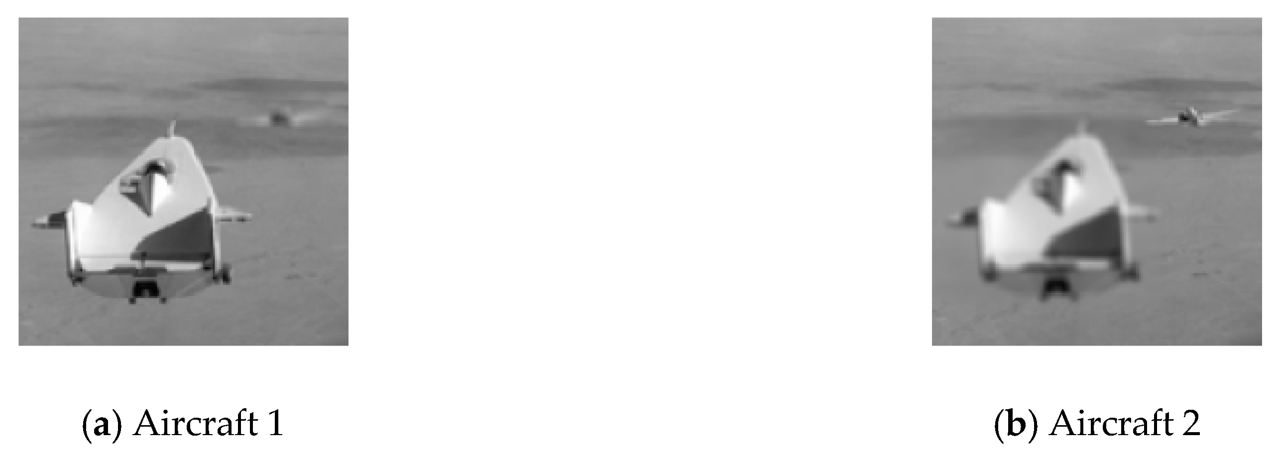
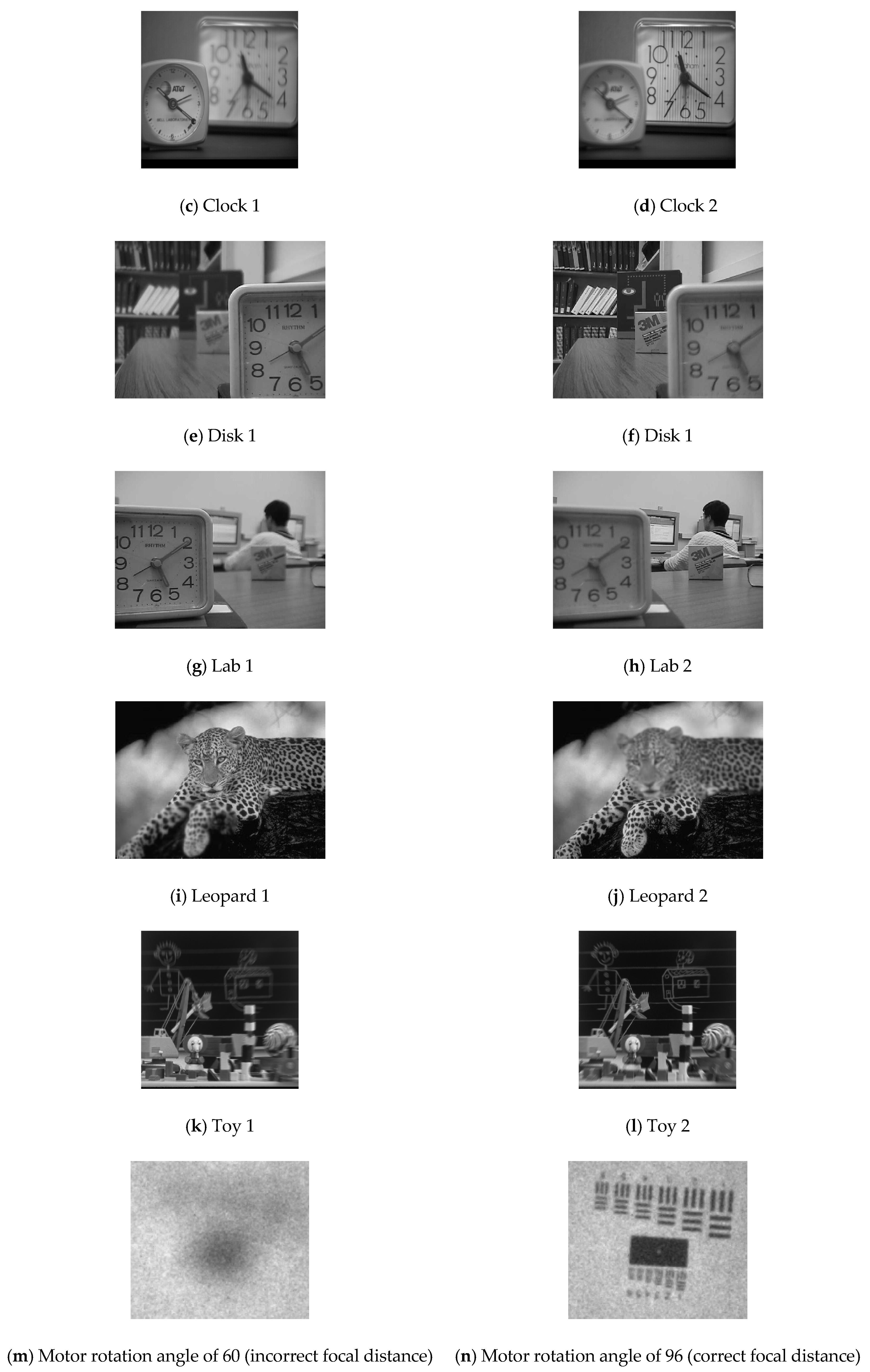
2.1. Description of Tested Images

In order to carry out various fusion method ratings, aircraft, clock, disk, lab, leopard, and toy images commonly used in research were used here to test the qualities of fusion methods. The images for testing were as shown in Figure 5a–l. In addition, the images for NVG testing of fusion results were as shown in Figure 5m,n. Through the aviaiton nighttime NVG testing bench (TS-3895A/UV) with NVG, the DC servo driver-driven focal knob was able to collect NVG testing images at the rotation angles ranging between 1 to 110 degrees. In order to simplify and facilitate the description of subsequent algorithms, the images collected were converted from colored ones into the gray-level, 110 images in total for autofocusing the algorithm used. To compare the quality of the traditional methods with the method in this paper, the same image sources as those of Jian and Peng [1] were used.

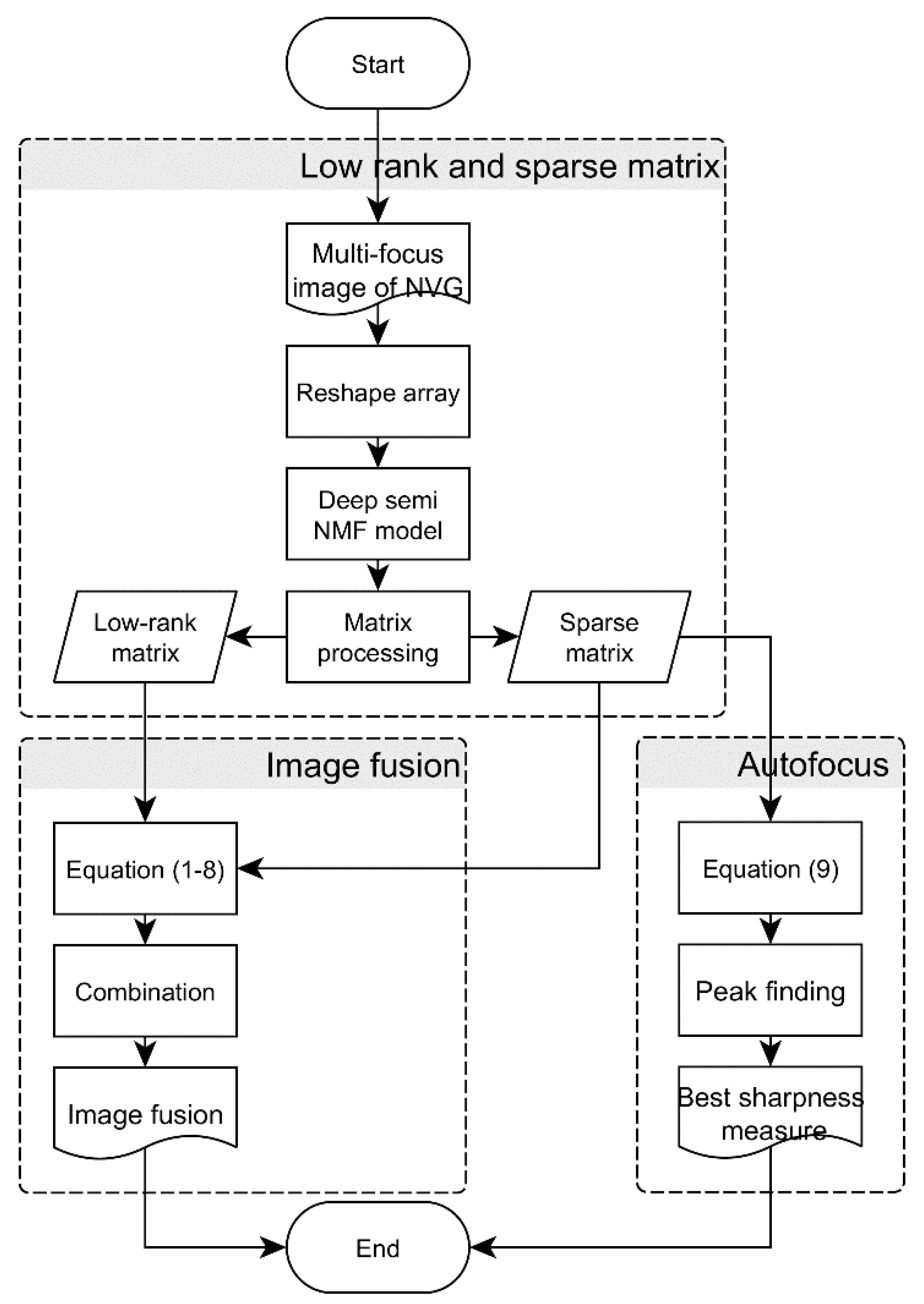
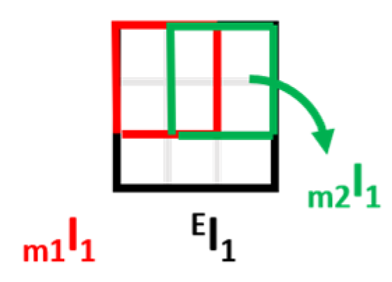
2.2. Image Fusion Using Low-Rank and Sparse Matrix

According to the fusion algorithm processing flow in Figure 4, the image fusion algorithm was verified. In the process, the diagram of a matrix structure of the source image for multifocus image of NVG was as shown in Figure 6. In particular, I is a two-dimenisonal image matrix, $t$ is the total number of images, the image height is $n$, and the width is m.

First, single source images were converted into one-dmeiensional vectors. Data arrangement in this step was as shown in Figure 7, where $I^R$ was a one-dimensional vector. Each one-dimensional vector $I_t^R$ was sequenced from top to bottom according to frame sequence. After combination, it was named D matrix (data matrix).

Then, the deep semi-NMF model method proposed by Trigeorgis, Bousmalis, Zafeiriou, and Schuller [34] was used here to obtain the low-dimensional representation. The equation is as shown in Equation (1):

$$D\approx Z\times H.$$

(1)

In particular, D is data matrix, Z is loadings matrix, and H is features matrix. This study adopted the method with low-dimesional characteristics to obtain A and E matrices. A is low-rank matrix and E is sparse matrix:

$$A=Z\times H,$$

(2)

$$E=D-A.$$

(3)

In A matrix, the relationship bewteen respective row vectors and images was as shown in Equation (4):

$$A=\left[\begin{array}{c}{}^{A}I{}_1^R\\ {}^{A}I{}_2^R\\ ⋮\\ {}^{A}I{}_t^R\end{array}\right],{}^{A}I{}_1^R:\mathrm{the}\mathrm{size}\mathrm{is}1\mathrm{by}\mathrm{L}$$

(4)

In particular, the length of $L\mathrm{is}n\times m$. In A matrix, the respective row vectors are, ${}^{A}I{}_1^R, {}^{A}I{}_2^R,\dots ,{}^{A}I{}_t^R$, respectively. In this paper, D matrix formed by respective images was decomposed into A and E matrices. Therefore, these two charactersitics were targeted for processing. In particular, A process involved reshaping the row vectors from ${}^{A}I{}_1^R$ through ${}^{A}I{}_t^R$ to the two-dimensional images of ${}^{A}I{}_1^{}-{}^{A}I{}_t^{}$ and obtaining the mean value. The result was called ${}^{A}I{}_{best}^{}$, and the process was as shown in Equation (5):

$${}^{A}I{}_{best}=\left({}^{A}I{}_1+{}^{A}I{}_2+\dots +{}^{A}I{}_t\right)/t$$

(5)

The first image corresponding to sparse matrix ${}^{E}I{}_1^{}$ and mask offset manipulation was as shown in Figure 8.

The corresponding image in sparse matrix was as shown in Equations (6) and (7):

$$OptIn{d}_z^x=\begin{array}{c}\arg \max \\ x\in \left[1, t\right]\end{array}\left(\mathrm{Var}\left({}_{m_z}I{}_x\right)\right), Z=1, 2, \dots ,len$$

(6)

$${}^{E}I{}_{best}={}^{E}I\left(OptInde{x}_z^x\right)$$

(7)

In particular, Var in Equation (6) is the computed variance, and $len$ is the total number of images undergoing mask offset. The best label obtained according to Equation (6) was used to acquire the ${}^{E}I{}_{best}^{}$ image in Equation (7), through which the best edge information was retained. Finally, the image obtained in Equation (5) was added to the images in ${}^{A}I{}_{best}^{}$ and Equation (7) to get the best fusion image $I_{best}$, as shown in Equation (8):

$$I_{best}={}^{A}I{}_{best}+{}^{E}I{}_{best}$$

(8)

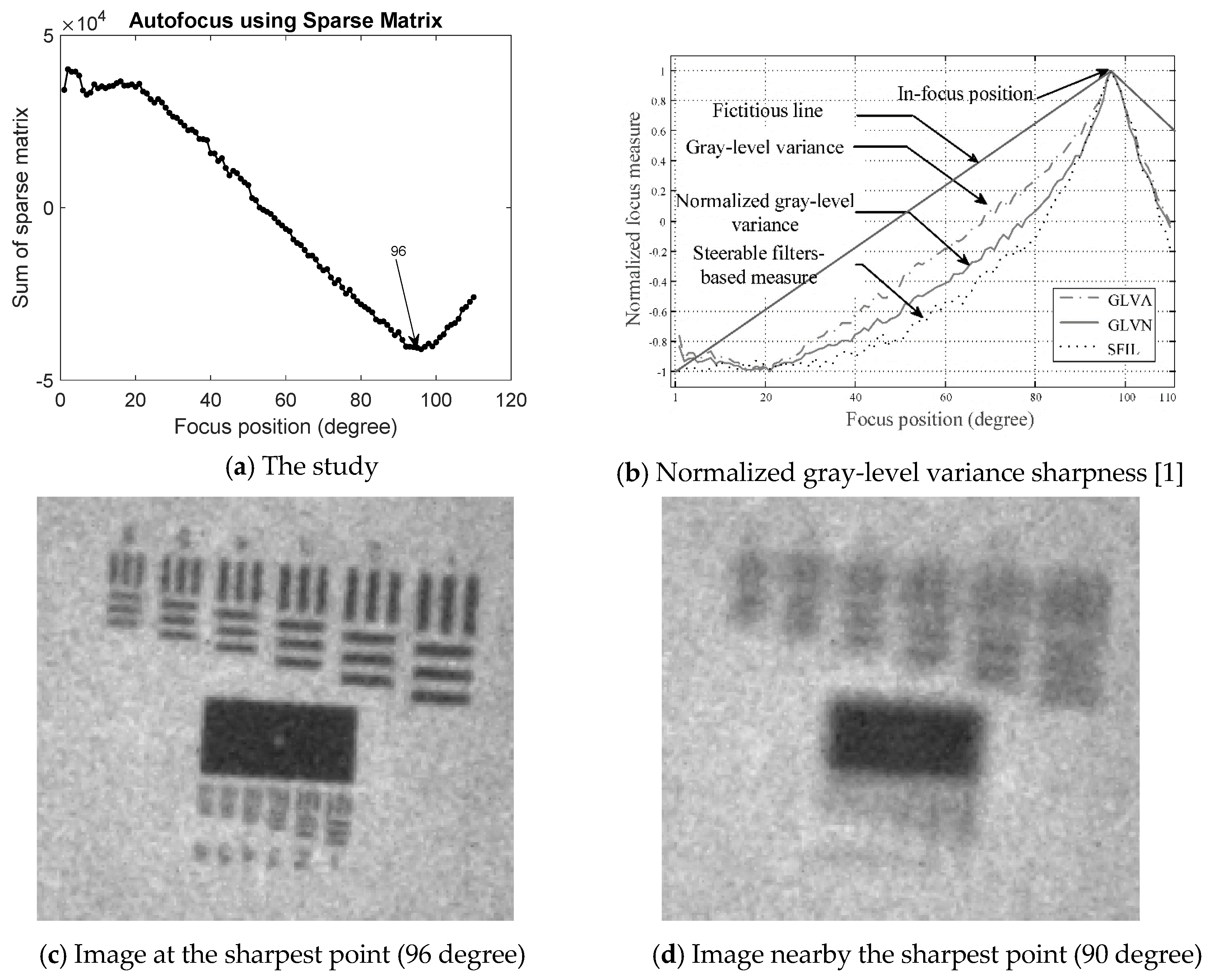
2.3. Autofocus Using Sparse Matrix

In addition to image fusion, autofocusing using sparse matrix method process was also put forward in this study. The sparse feature of sparse matrix was mainly used to test the focus stripe correlation generated from the testing bench. Since low-rank matrix had the main components of focus stripe, it had the same signficiance pointed out in Equation (3) where sparse matrix was the orignal image subtracted by low-rank matrix. Hence, the correpsonding frame information in sparse matrix can be used as a reference for sharpness. This concept was applied in the acutal practice. First, 110 images of different focal distances were compiled into D matrix accoridng to the arrangement diagram in Figure 6 and Figure 7. As shown in Equations (1) through (4), they were decomposed into low-rank matrix A and sparse matrix E. Then, ${}^{E}I{}_i^R ,$ i = 1,2,3…t corrsponding to different focal distances in E matrix were directly used to calulate the images corresponding to single ${}^{E}I{}_i^R ,$ to tally the results. An image frame corresponding to the lowest value was the sharpest frame. In particular, the lowest point in Figure 4 was the frame with the best sharpness. The calculation can be simplified into Equation (9).

$$\begin{array}{cc}\hfill FP& =\begin{array}{c}\arg \min \\ i\in \left[1, t\right]\end{array}\left({\displaystyle {\displaystyle \sum }_{k=1}^N}{}^{E}I{}_i^R\left(k\right)\right)\hfill \\ & =\begin{array}{c}\arg \min \\ i\in \left[1, t\right]\end{array}\left({\displaystyle {\displaystyle \sum }_{x=1}^m}{\displaystyle {\displaystyle \sum }_{y=1}^n}{}^{E}I{}_i\left(x,y\right)\right)\hfill \end{array}$$

(9)

where FP is focus position and N = m × n is image size.

3. Experiment Results and Discussion

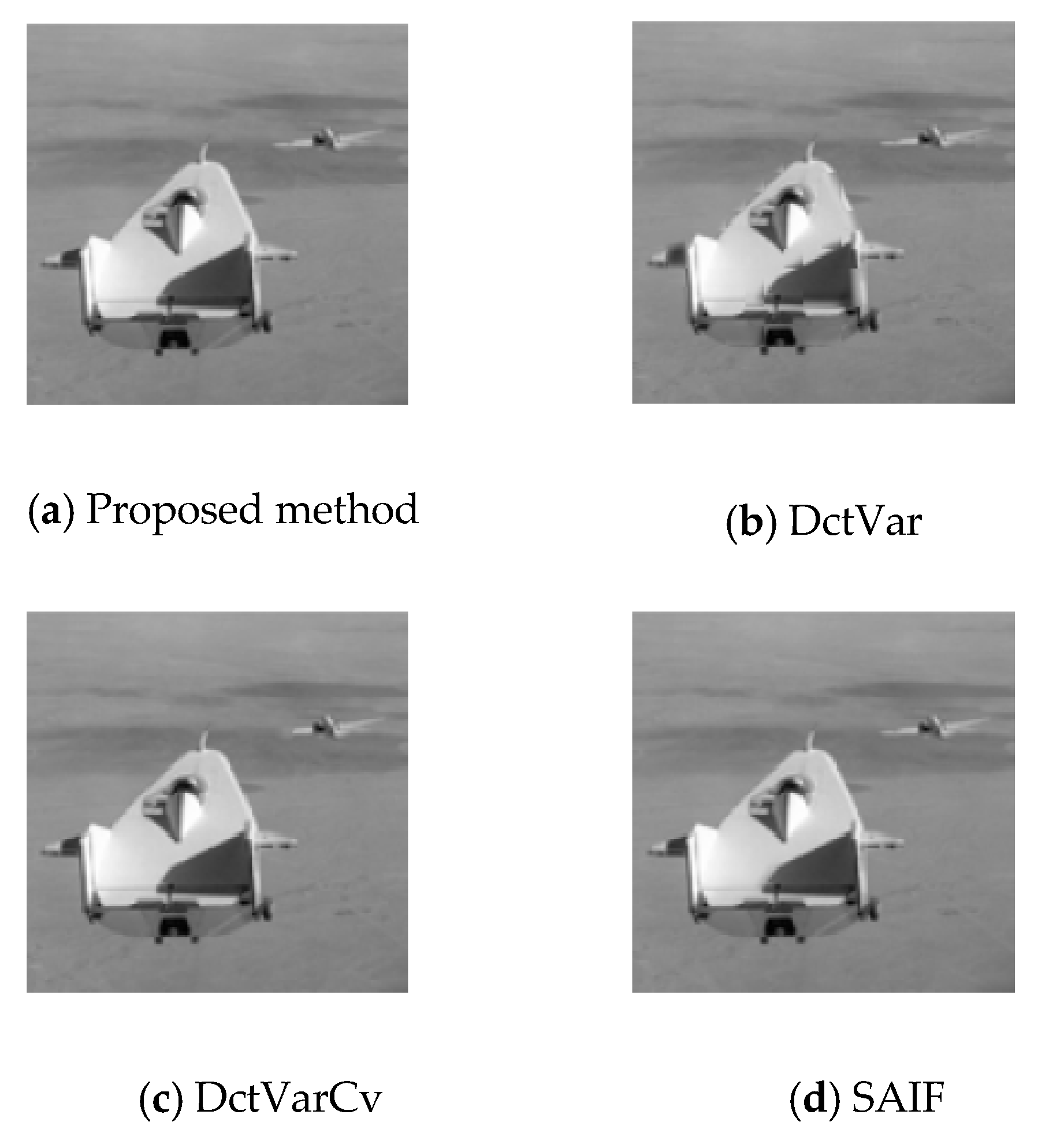
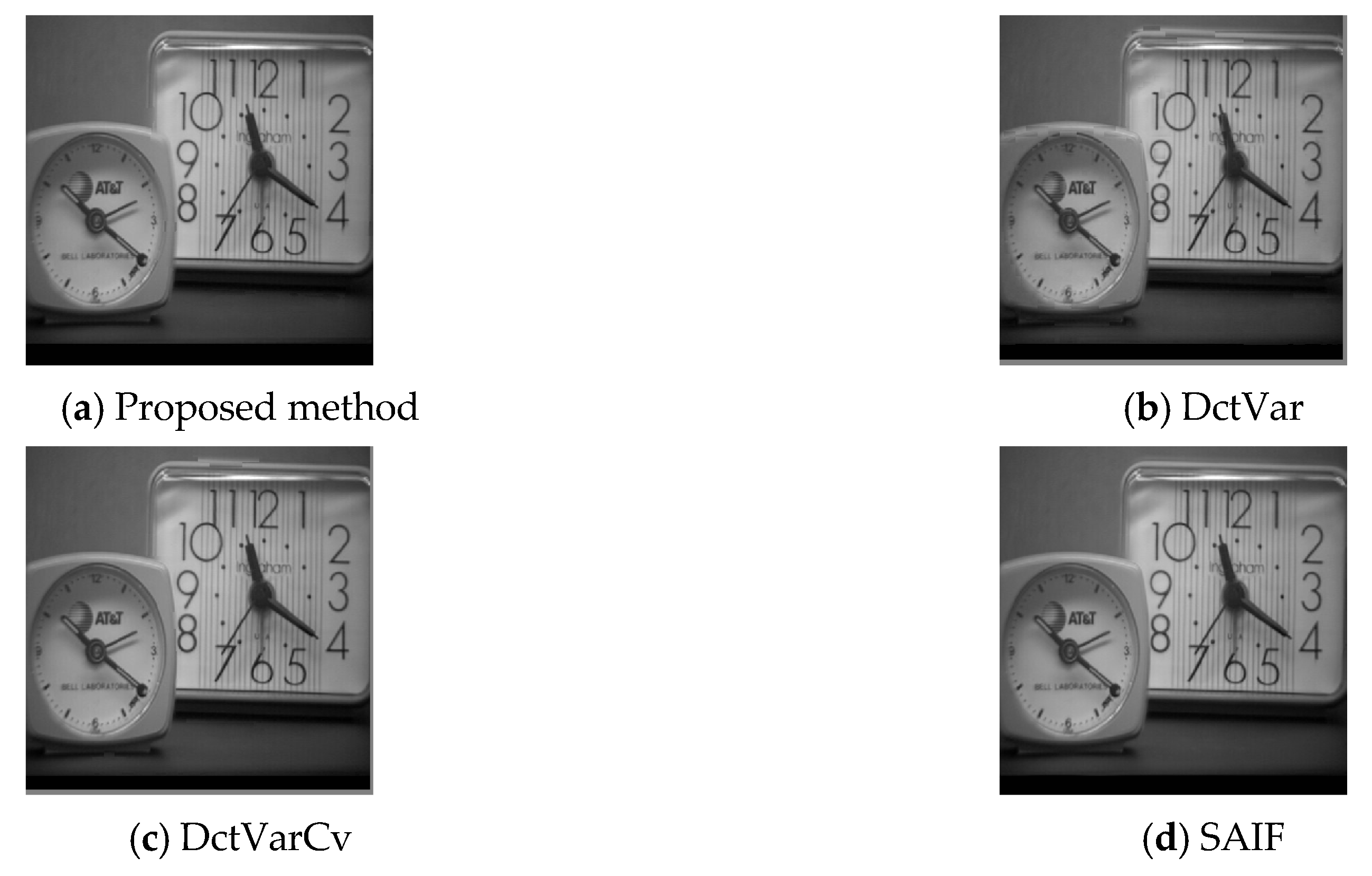
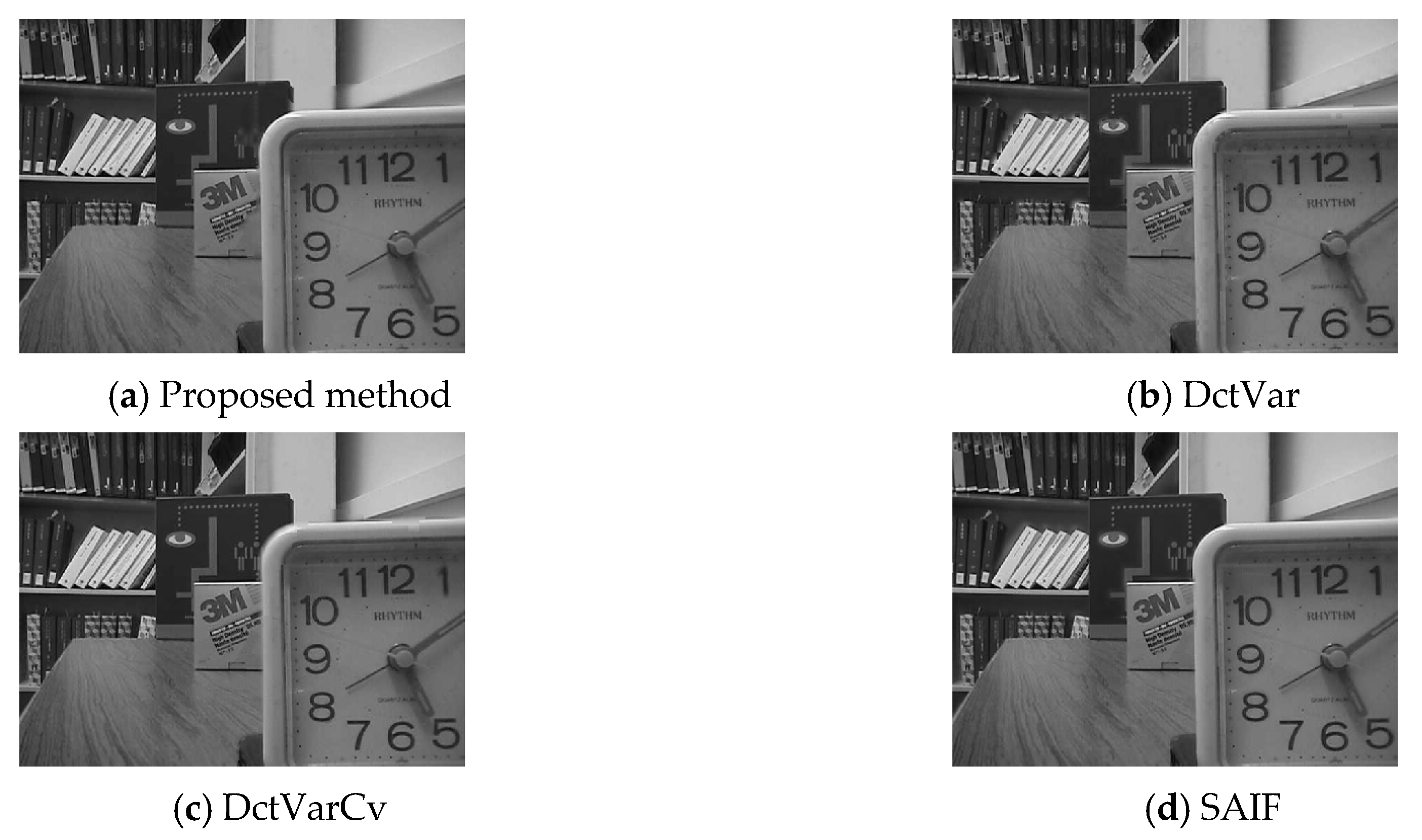
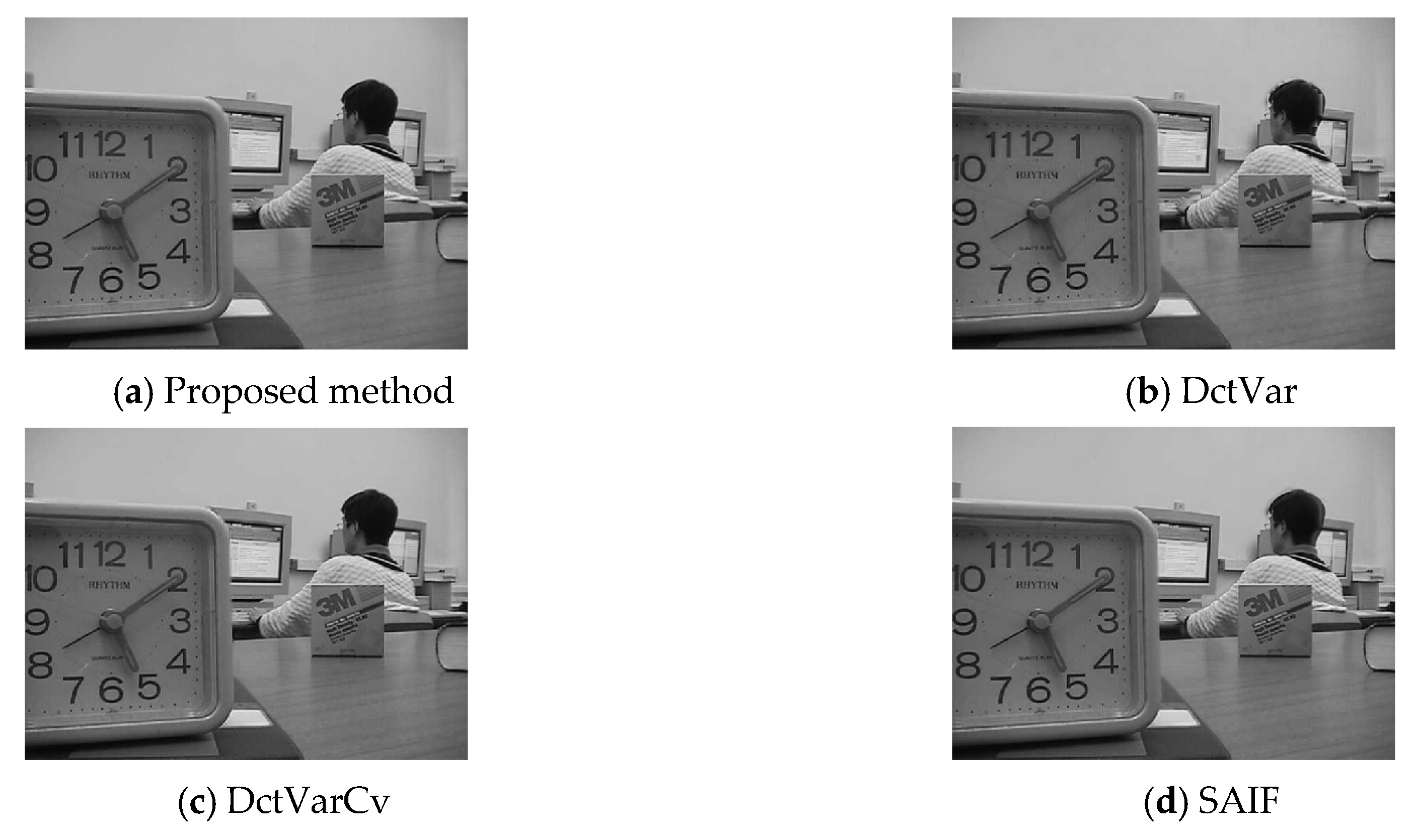
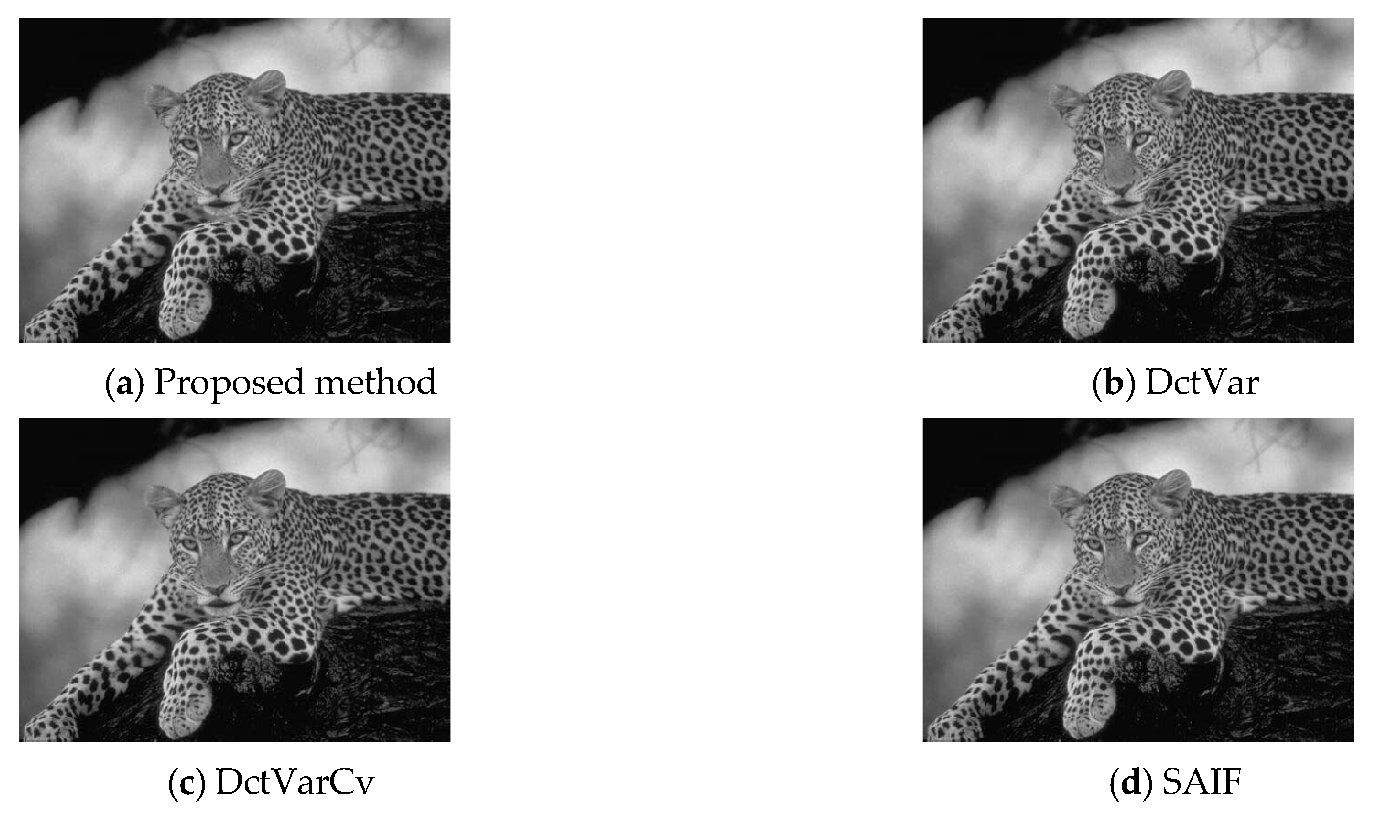
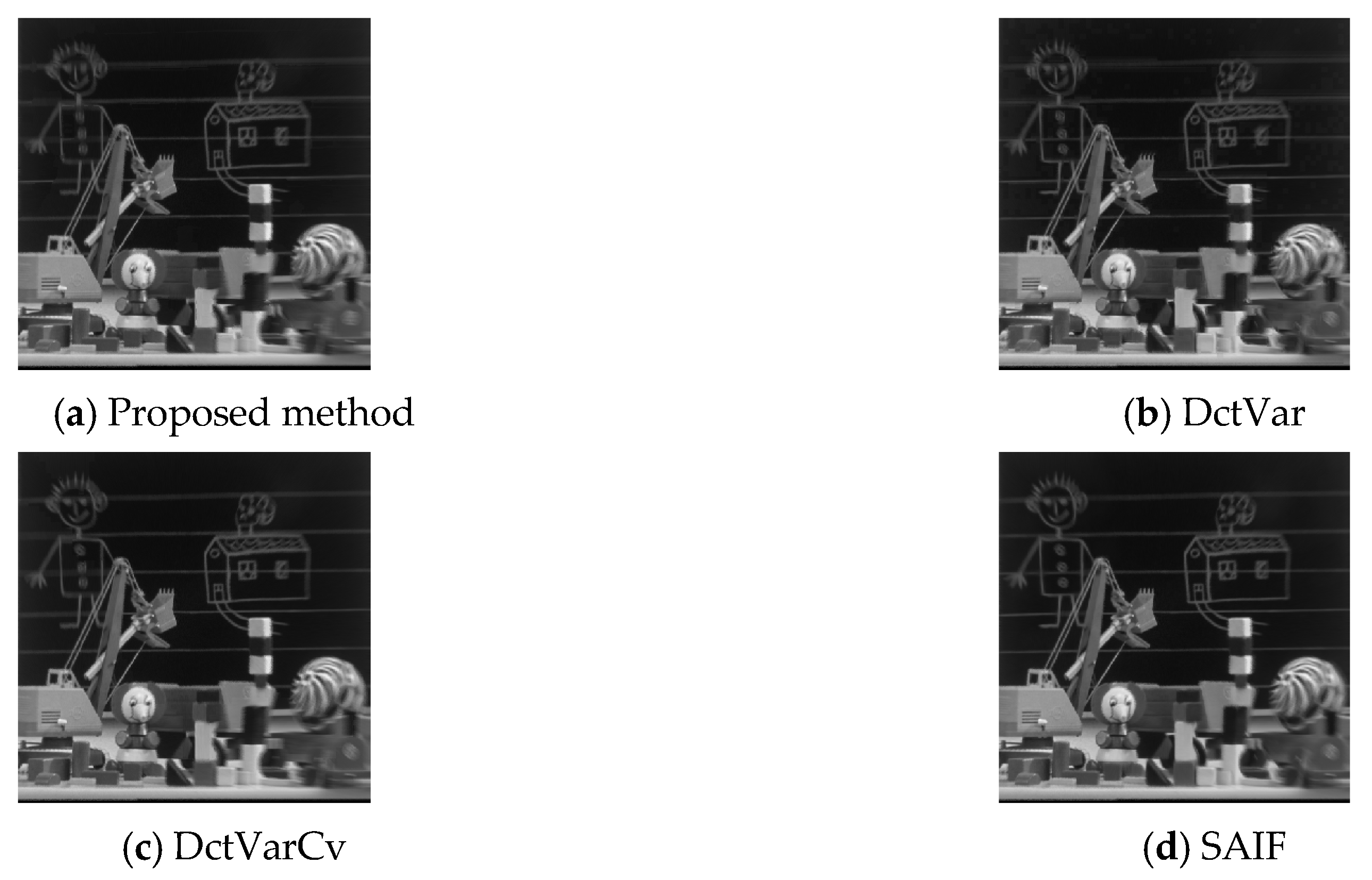
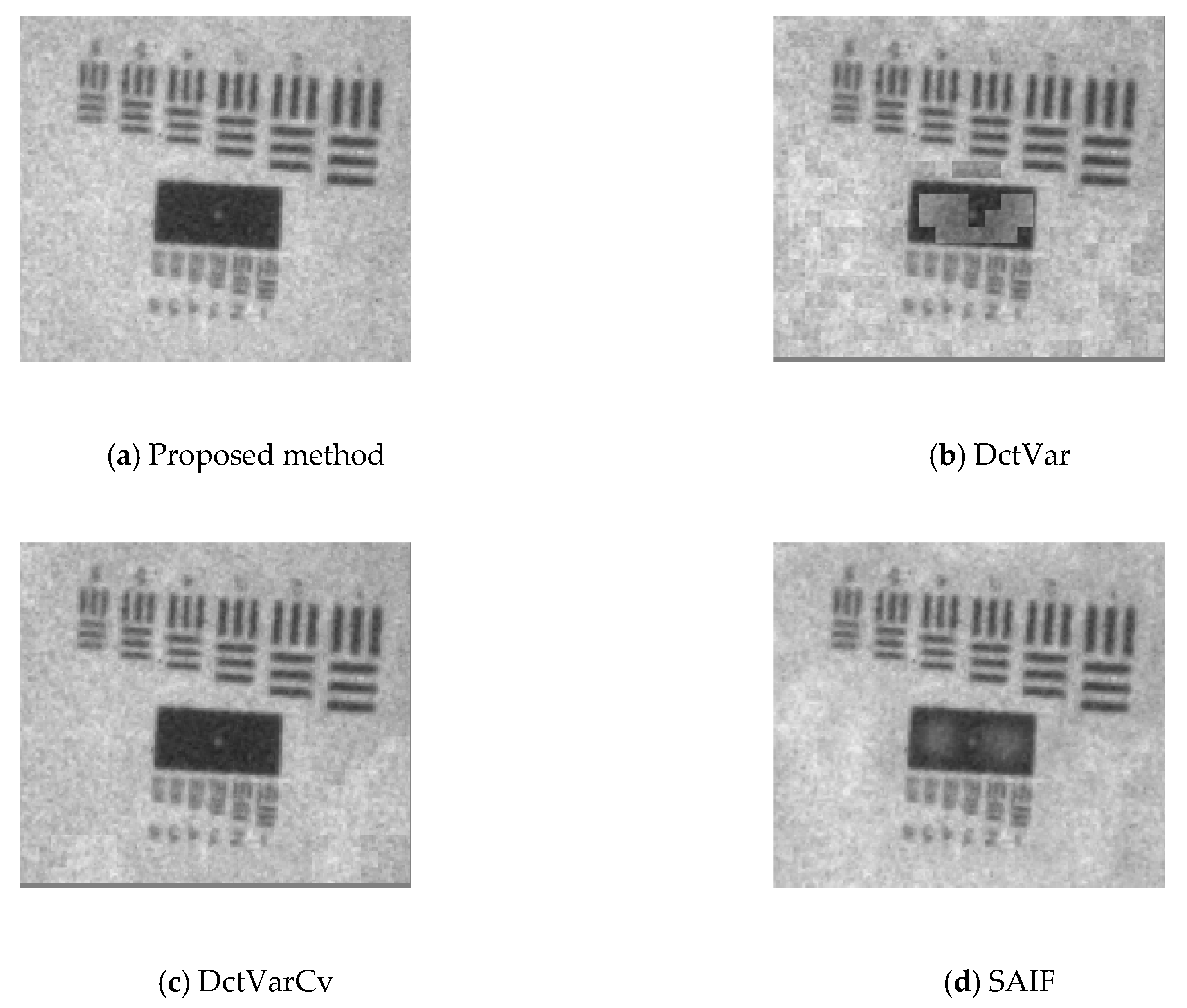
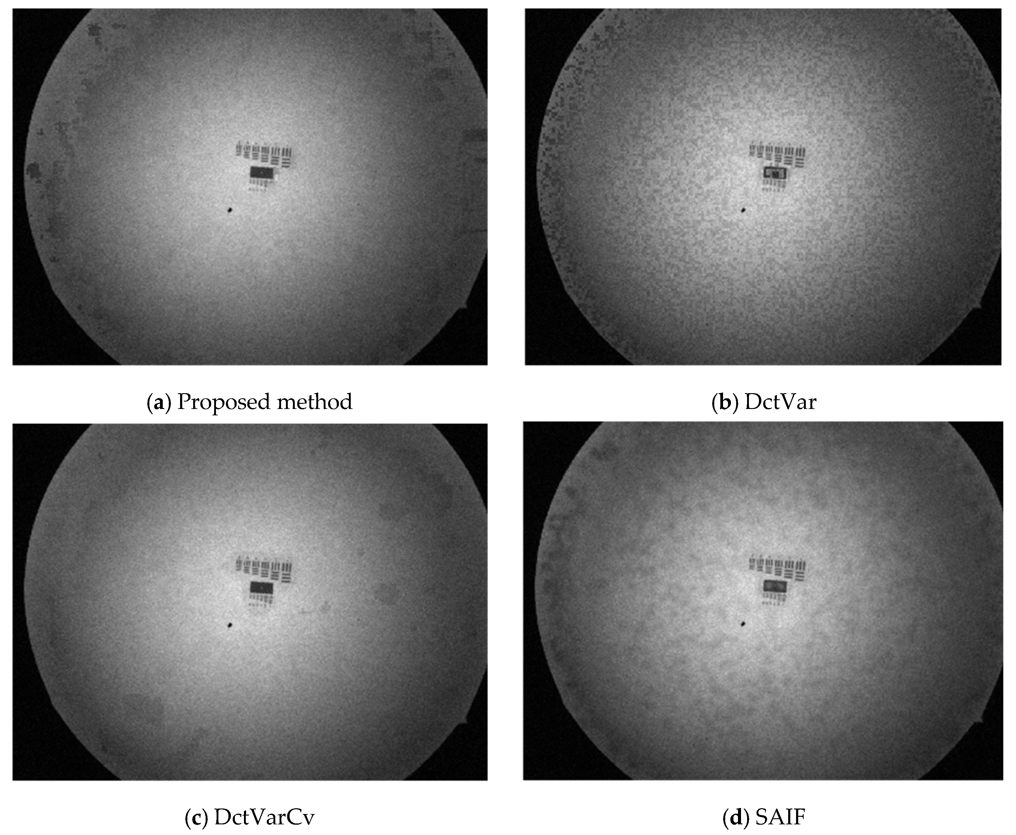
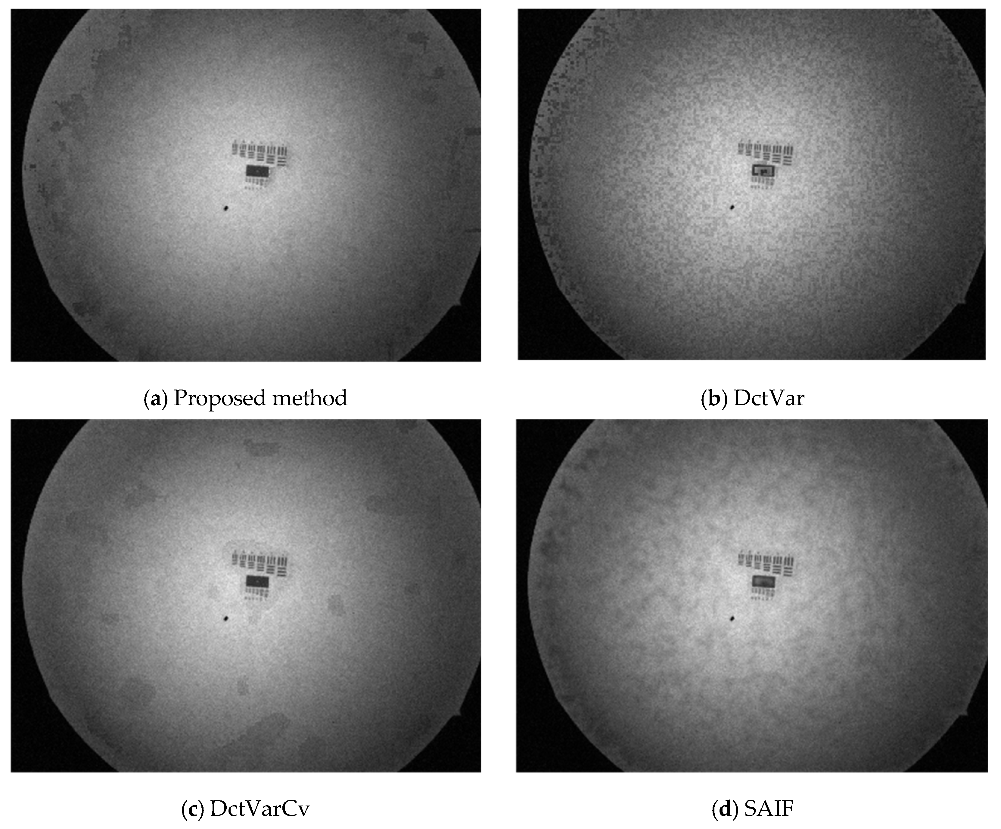
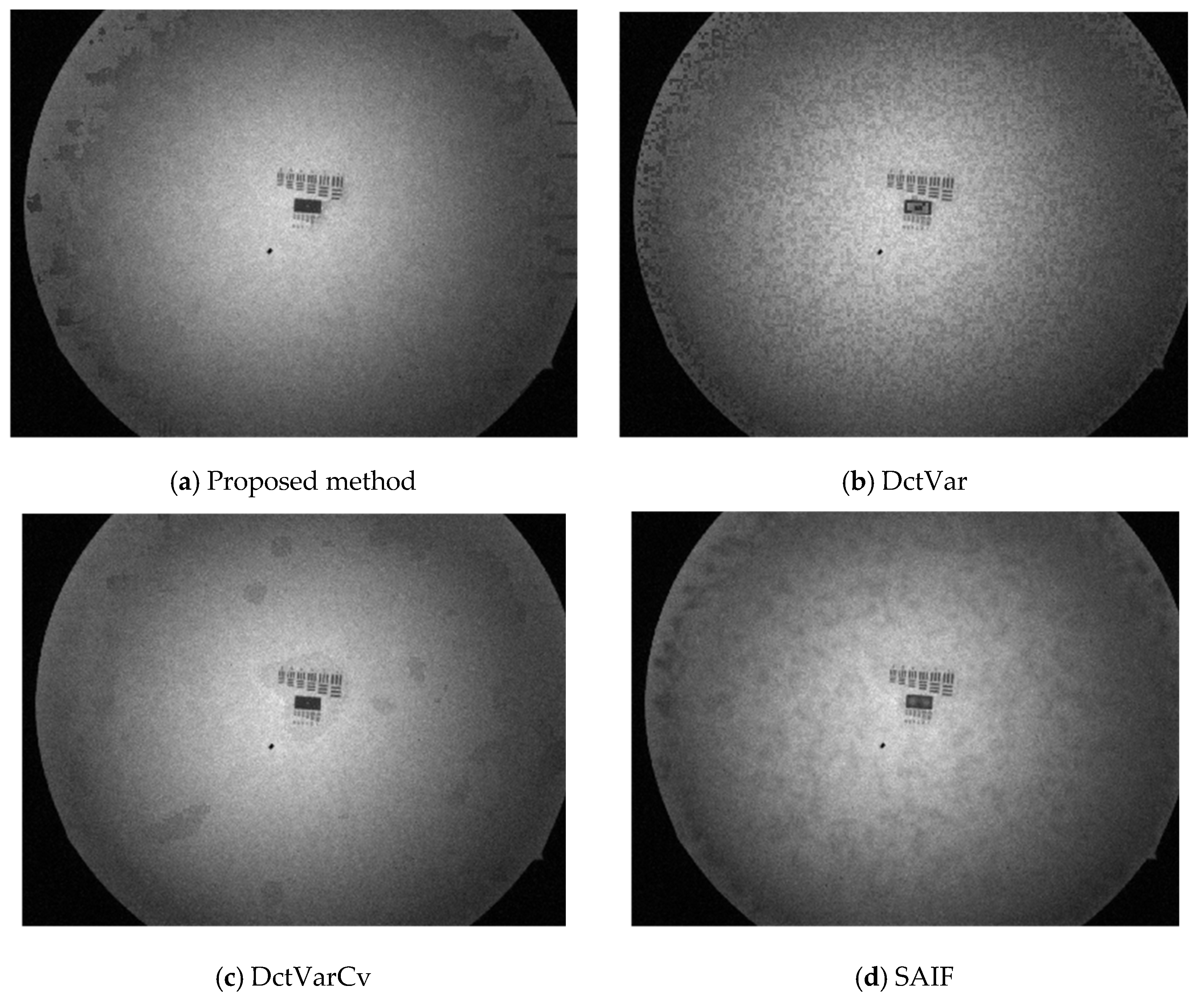
3.1. Image Fusion Results

According to the image fusion method propsed in Figure 4 and the based-on variance calculated in discrete cosine transform domain without consistency verification (DctVar) and based-on variance calculated in discrete cosine transform domain with consistency verification (DctVarCv) [12,13] and structure-aware image fusion (SAIF) [11] methods, comparison and verification were carried out. This study was to evaluate the quality of image fusion using relevant indicators compiled by Liu et al. [42]. The original images verified were as shown in the description of the tested images section. The fusion results of the respective images were as shown from Figure 9, Figure 10, Figure 11, Figure 12, Figure 13 and Figure 14. Among which, (a) is the mehtod proposed in this study, (b) is the fused image result of DctVar method, (c) is the fused image result of DctVarCv method, and (d) is the fused image result of SAIF method. The fusion indicator results of vairous images were as shown from

Table 1. List of aircraft fusion results and fusion quality indicators.

Aircraft	Proposed Method	DctVar	DctVarCv	SAIF	Optimum
$Q_{\mathrm{MI}}$	1.37	1.32	1.36	1.31	This study (4) > DctVarCv (3) > DctVar (2) > SAIF (1)
$Q_{\mathrm{TE}}$	0.442	0.434	0.441	0.441	This study (4) > DctVarCv (3) > SAIF (2) > DctVar (1)
$Q_{\mathrm{NCIE}}$	0.847	0.842	0.845	0.842	This study (4) > DctVarCv (3) > DctVar (2) > SAIF (1)
$Q_G$	0.672	0.648	0.674	0.662	DctVarCv (4) > This study (3) > SAIF (2) > DctVar (1)
$Q_M$	2.312	2.253	2.311	2.082	This study (4) > DctVarCv (3) > DctVar (2) > SAIF (1)
$Q_{\mathrm{SF}}$	-0.059	-0.091	-0.060	-0.068	This study (4) > DctVarCv (3) > SAIF (2) > DctVar (1)
$Q_P$	0.79	0.7	0.80	0.78	DctVarCv (4) > This study (3) > SAIF (2) > DctVar (1)
$Q_S$	0.948	0.948	0.948	0.953	SAIF (4) > DctVar (3) > This study (2) > DctVarCv (1)
$Q_C$	0.89	0.83	0.88	0.88	This study (4) > DctVarCv (3) > SAIF (2) > DctVar (1)
$Q_Y$	0.974	0.931	0.977	0.965	DctVarCv (4) > This study (3) > SAIF (2) > DctVar (1)
$Q_{\mathrm{CV}}$	9	18	9	9	DctVar (4) > This study (3) > DctVarCv (2) > SAIF (1)
$Q_{\mathrm{CB}}$	0.7597	0.709	0.76	0.745	DctVarCv (4) > This study (3) > SAIF (2) > DctVar (1)
Total score	41	20	37	22

Optimum rule: Index headed the table with maximum points. Normalized mutual information ($Q_{\mathrm{MI}}$); Fusion metric based on Tsallis entropy ($Q_{\mathrm{TE}}$); Nonlinear correlation information entropy ($Q_{\mathrm{NCIE}}$); Gradient-based fusion performance ($Q_G$); Image fusion metric based on a multiscale scheme ($Q_M$); Image fusion metric based on spatial frequency ($Q_{\mathrm{SF}}$); Image fusion metric based on phase congruency ($Q_P$); Piella’s metric ($Q_S$); Cvejie’s metric ($Q_C$); Yang’s metric ($Q_Y$); Chen–Varshney metric ($Q_{\mathrm{CV}}$); Chen–Blum metric ($Q_{\mathrm{CB}}$).

,

Table 2. List of clock fusion results and fusion quality indicators.

Clock	Proposed Method	DctVar	DctVarCv	SAIF	Optimum
$Q_{\mathrm{MI}}$	1.21	1.18	1.19	1.14	This study (4) > DctVarCv (3) > DctVar (2) > SAIF (1)
$Q_{\mathrm{TE}}$	0.415	0.406	0.41	0.411	This study (4) > SAIF (3) > DctVarCv (2) > DctVar (1)
$Q_{\mathrm{NCIE}}$	0.8447	0.8424	0.8441	0.8398	This study (4) > DctVarCv (3) > DctVar (2) > SAIF (1)
$Q_G$	0.682	0.662	0.68	0.676	This study (4) > DctVarCv (3) > SAIF (2) > DctVar (1)
$Q_M$	2.56	2.58	2.6	2.35	DctVarCv (4) > DctVar (3) > This study (2) > SAIF (1)
$Q_{\mathrm{SF}}$	-0.04	0.17	0.16	-0.06	DctVar (4) > DctVarCv (3) > This study (2) > SAIF (1)
$Q_P$	0.804	0.629	0.739	0.803	This study (4) > SAIF (3) > DctVarCv (2) > DctVar (1)
$Q_S$	0.946	0.926	0.933	0.956	SAIF (4) > This study (3) > DctVarCv (2) > DctVar (1)
$Q_C$	0.798	0.756	0.77	0.801	SAIF (4) > This study (3) > DctVarCv (2) > DctVar (1)
$Q_Y$	0.98	0.9	0.96	0.96	This study (4) > SAIF (3) > DctVarCv (2) > DctVar (1)
$Q_{\mathrm{CV}}$	13	104	98	12	DctVar (4) > DctVarCv (3) > This study (2) > SAIF (1)
$Q_{\mathrm{CB}}$	0.77	0.65	0.72	0.75	This study (4) > SAIF (3) > DctVarCv (2) > DctVar (1)
Total score	40	22	31	27

Optimum rule: Index headed the table with maximum points. Normalized mutual information ($Q_{\mathrm{MI}}$); Fusion metric based on Tsallis entropy ($Q_{\mathrm{TE}}$); Nonlinear correlation information entropy ($Q_{\mathrm{NCIE}}$); Gradient-based fusion performance ($Q_G$); Image fusion metric based on a multiscale scheme ($Q_M$); Image fusion metric based on spatial frequency ($Q_{\mathrm{SF}}$); Image fusion metric based on phase congruency ($Q_P$); Piella’s metric ($Q_S$); Cvejie’s metric ($Q_C$); Yang’s metric ($Q_Y$); Chen–Varshney metric ($Q_{\mathrm{CV}}$); Chen–Blum metric ($Q_{\mathrm{CB}}$).

,

Table 3. List of disk fusion results and fusion quality indicators.

Disk	Proposed Method	DctVar	DctVarCv	SAIF	Optimum
$Q_{\mathrm{MI}}$	1.12	1.11	1.15	1	DctVarCv (4) > This study (3) > DctVar (2) > SAIF (1)
$Q_{\mathrm{TE}}$	0.384	0.372	0.387	0.373	DctVarCv (4) > This study (3) > SAIF (2) > DctVar (1)
$Q_{\mathrm{NCIE}}$	0.836	0.837	0.84	0.831	DctVarCv (4) > DctVar (3) > This study (2) > SAIF (1)
$Q_G$	0.68	0.7	0.69	0.68	DctVar (4) > DctVarCv (3) > SAIF (2) > This study (1)
$Q_M$	2.3	2.8	2.7	2.2	DctVar (4) > DctVarCv (3) > This study (2) > SAIF (1)
$Q_{\mathrm{SF}}$	-0.04	-0.01	-0.04	-0.04	DctVar (4) > DctVarCv (3) > This study (2) > SAIF (1)
$Q_P$	0.777	0.666	0.795	0.797	SAIF (4) > DctVarCv (3) > This study (2) > DctVar (1)
$Q_S$	0.92	0.92	0.92	0.93	SAIF (4) > DctVarCv (3) > DctVar (2) > This study (1)
$Q_C$	0.769	0.746	0.756	0.766	This study (4) > SAIF (3) > DctVarCv (2) > DctVar (1)
$Q_Y$	0.983	0.919	0.989	0.956	DctVarCv (4) > This study (3) > SAIF (2) > DctVar (1)
$Q_{\mathrm{CV}}$	13	142	27	17	DctVar (4) > DctVarCv (3) > SAIF (2) > This study (1)
$Q_{\mathrm{CB}}$	0.76	0.68	0.78	0.73	DctVarCv (4) > This study (3) > SAIF (2) > DctVar (1)
Total score	27	28	40	25

Optimum rule: Index headed the table with maximum points. Normalized mutual information ($Q_{\mathrm{MI}}$); Fusion metric based on Tsallis entropy ($Q_{\mathrm{TE}}$); Nonlinear correlation information entropy ($Q_{\mathrm{NCIE}}$); Gradient-based fusion performance ($Q_G$); Image fusion metric based on a multiscale scheme ($Q_M$); Image fusion metric based on spatial frequency ($Q_{\mathrm{SF}}$); Image fusion metric based on phase congruency ($Q_P$); Piella’s metric ($Q_S$); Cvejie’s metric ($Q_C$); Yang’s metric ($Q_Y$); Chen–Varshney metric ($Q_{\mathrm{CV}}$); Chen–Blum metric ($Q_{\mathrm{CB}}$).

,

Table 4. List of leopard fusion results and fusion quality indicators.

Leopard	Proposed Method	DctVar	DctVarCv	SAIF	Optimum
$Q_{\mathrm{MI}}$	1.4509	1.4708	1.471	1.4631	DctVarCv (4) > DctVar (3) > SAIF (2) > This study (1)
$Q_{\mathrm{TE}}$	0.4598	0.4524	0.4539	0.4601	SAIF (4) > This study (3) > DctVarCv (2) > DctVar (1)
$Q_{\mathrm{NCIE}}$	0.8677	0.8695	0.8692	0.8688	DctVar (4) > DctVarCv (3) > SAIF (2) > This study (1)
$Q_G$	0.856	0.857	0.857	0.859	SAIF (4) > DctVarCv (3) > DctVar (2) > This study (1)
$Q_M$	2.476	2.7	2.695	2.667	DctVar (4) > DctVarCv (3) > SAIF (2) > This study (1)
$Q_{\mathrm{SF}}$	-0.0133	-0.0116	-0.0118	-0.0113	SAIF (4) > DctVar (3) > DctVarCv (2) > This study (1)
$Q_P$	0.947	0.947	0.949	0.952	SAIF (4) > DctVarCv (3) > This study (2) > DctVar (1)
$Q_S$	0.9734	0.9737	0.9737	0.9742	SAIF (4) > DctVar (3) > DctVarCv (2) > This study (1)
$Q_C$	0.945	0.944	0.945	0.946	SAIF (4) > This study (3) > DctVarCv (2) > DctVar (1)
$Q_Y$	0.9923	0.9904	0.9921	0.9929	SAIF (4) > This study (3) > DctVarCv (2) > DctVar (1)
$Q_{\mathrm{CV}}$	13.2	13.8	13.4	12.7	DctVar (4) > DctVarCv (3) > This study (2) > SAIF (1)
$Q_{\mathrm{CB}}$	0.836	0.872	0.874	0.844	DctVarCv (4) > DctVar (3) > SAIF (2) > This study (1)
Total score	20	30	33	37

Optimum rule: Index headed the table with maximum points. Normalized mutual information ($Q_{\mathrm{MI}}$); Fusion metric based on Tsallis entropy ($Q_{\mathrm{TE}}$); Nonlinear correlation information entropy ($Q_{\mathrm{NCIE}}$); Gradient-based fusion performance ($Q_G$); Image fusion metric based on a multiscale scheme ($Q_M$); Image fusion metric based on spatial frequency ($Q_{\mathrm{SF}}$); Image fusion metric based on phase congruency ($Q_P$); Piella’s metric ($Q_S$); Cvejie’s metric ($Q_C$); Yang’s metric ($Q_Y$); Chen–Varshney metric ($Q_{\mathrm{CV}}$); Chen–Blum metric ($Q_{\mathrm{CB}}$).

,

Table 5. List of lab fusion results and fusion quality indicators.

Lab	Proposed Method	DctVar	DctVarCv	SAIF	Optimum
$Q_{\mathrm{MI}}$	1.26	1.22	1.27	1.18	DctVarCv (4) > This study (3) > DctVar (2) > SAIF (1)
$Q_{\mathrm{TE}}$	0.43	0.417	0.427	0.418	This study (4) > DctVarCv (3) > SAIF (2) > DctVar (1)
$Q_{\mathrm{NCIE}}$	0.843	0.841	0.844	0.839	DctVarCv (4) > This study (3) > DctVar (2) > SAIF (1)
$Q_G$	0.73	0.74	0.73	0.72	DctVar (4) > DctVarCv (3) > This study (2) > SAIF (1)
$Q_M$	2.34	2.7	2.695	2.398	DctVar (4) > DctVarCv (3) > SAIF (2) > This study (1)
$Q_{\mathrm{SF}}$	-0.03	-0.01	-0.03	-0.03	DctVar (4) > DctVarCv (3) > This study (2) > SAIF (1)
$Q_P$	0.784	0.674	0.799	0.795	DctVarCv (4) > SAIF (3) > This study (2) > DctVar (1)
$Q_S$	0.95	0.948	0.951	0.956	SAIF (4) > DctVarCv (3) > This study (2) > DctVar (1)
$Q_C$	0.802	0.786	0.798	0.791	This study (4) > DctVarCv (3) > SAIF (2) > DctVar (1)
$Q_Y$	0.98	0.92	1	0.95	DctVarCv (4) > This study (3) > SAIF (2) > DctVar (1)
$Q_{\mathrm{CV}}$	5	18	5	8	DctVar (4) > SAIF (3) > This study (2) > DctVarCv (1)
$Q_{\mathrm{CB}}$	0.72	0.65	0.76	0.72	DctVarCv (4) > This study (3) > SAIF (2) > DctVar (1)
Total score	31	26	39	24

Optimum rule: Index headed the table with maximum points. Normalized mutual information ($Q_{\mathrm{MI}}$); Fusion metric based on Tsallis entropy ($Q_{\mathrm{TE}}$); Nonlinear correlation information entropy ($Q_{\mathrm{NCIE}}$); Gradient-based fusion performance ($Q_G$); Image fusion metric based on a multiscale scheme ($Q_M$); Image fusion metric based on spatial frequency ($Q_{\mathrm{SF}}$); Image fusion metric based on phase congruency ($Q_P$); Piella’s metric ($Q_S$); Cvejie’s metric ($Q_C$); Yang’s metric ($Q_Y$); Chen–Varshney metric ($Q_{\mathrm{CV}}$); Chen–Blum metric ($Q_{\mathrm{CB}}$).

and

Table 6. List of toy fusion results and fusion quality indicators.

Toy	Proposed Method	DctVar	DctVarCv	SAIF	Optimum
$Q_{\mathrm{MI}}$	1.17	1.16	1.2	1.06	DctVarCv (4) > This study (3) > DctVar (2) > SAIF (1)
$Q_{\mathrm{TE}}$	0.431	0.419	0.43	0.436	SAIF (4) > This study (3) > DctVarCv (2) > DctVar (1)
$Q_{\mathrm{NCIE}}$	0.836	0.836	0.837	0.831	DctVarCv (4) > This study (3) > DctVar (2) > SAIF (1)
$Q_G$	0.63	0.62	0.65	0.63	DctVarCv (4) > This study (3) > SAIF (2) > DctVar (1)
$Q_M$	1.5	2.1	2	1.7	DctVar (4) > DctVarCv (3) > SAIF (2) > This study (1)
$Q_{\mathrm{SF}}$	-0.11	-0.08	-0.11	-0.11	DctVar (4) > DctVarCv (3) > SAIF (2) > This study (1)
$Q_P$	0.771	0.695	0.824	0.821	DctVarCv (4) > SAIF (3) > This study (2) > DctVar (1)
$Q_S$	0.934	0.931	0.936	0.948	SAIF (4) > DctVarCv (3) > This study (2) > DctVar (1)
$Q_C$	0.8	0.756	0.823	0.816	DctVarCv (4) > SAIF (3) > This study (2) > DctVar (1)
$Q_Y$	0.94	0.86	0.98	0.95	DctVarCv (4) > SAIF (3) > This study (2) > DctVar (1)
$Q_{\mathrm{CV}}$	32	35	31	29	DctVar (4) > This study (3) > DctVarCv (2) > SAIF (1)
$Q_{\mathrm{CB}}$	0.73	0.66	0.77	0.76	DctVarCv (4) > SAIF (3) > This study (2) > DctVar (1)
Total score	27	23	41	29

Optimum rule: Index headed the table with maximum points. Normalized mutual information ($Q_{\mathrm{MI}}$); Fusion metric based on Tsallis entropy ($Q_{\mathrm{TE}}$); Nonlinear correlation information entropy ($Q_{\mathrm{NCIE}}$); Gradient-based fusion performance ($Q_G$); Image fusion metric based on a multiscale scheme ($Q_M$); Image fusion metric based on spatial frequency ($Q_{\mathrm{SF}}$); Image fusion metric based on phase congruency ($Q_P$); Piella’s metric ($Q_S$); Cvejie’s metric ($Q_C$); Yang’s metric ($Q_Y$); Chen–Varshney metric ($Q_{\mathrm{CV}}$); Chen–Blum metric ($Q_{\mathrm{CB}}$).

. Among these four fusion methods, gray background’s fusion quality indicator pointed out the best results for the 12 indicators, which in seuqence were: $Q_{\mathrm{MI}}$, $Q_{\mathrm{TE}}$, $Q_{\mathrm{NCIE}}$, $Q_G$, $Q_M$, $Q_{\mathrm{SF}}$, $Q_P$, $Q_S$, $Q_C$, $Q_Y$, $Q_{\mathrm{CV}}$, $Q_{\mathrm{CB}}$. The higher the value, the better the fusion quality.

3.2. Image Fusion Results of the Discussion

In the air craft image fusion result, seven indicators point out that the method in this study derived the best fusion result. From the subjective human eye observation, it was deemed that the fusion result using the DctVar method was clearly the poorest, while the other results were more approximate. In the clock image fusion result, the seven indicdators showed the study derived the best fusion result, while the subjective human eye observation deemed the DctVar and DctVarCv results to be the poorest. The study and the SAIF methods were equally matched in terms of the details. In the disk image fusion result, the five indicators showed the DctVarCv method derived the best fusion result, while the subejctive human eye observation deemed the DctVar and DctVarCv reuslts to be the poorest. The square effect clearly existed in the images. On the other hand, the SAIF method derived the best fusion result. There was a considerable difference between the indicator reuslts and the human eye congition. It was speculated that the square effect exerted less influence on the ratings of the indicdators. In the lab image fusion results, the five indicators showed the DctVarCv derived the best fusion results. The subejctive human eye observation deemed DctVar and SAIF results to be the poorest, with suqare effect and halo lines in the head region. The DctVarCv and the study derived the best fusion results. In the leopard image fusion results, the seven indicadtors showed SAIF derived the best fusion result, but the respecitve indidactors were basically quite approximate. The subjecitve eye observation deemed the respective methods derived the same results. In the toy image fusion results, the six indicators sshowed DctVarCv derived the best fusion result. The subejctive eye observation deemed the study and SAIF derived the best fusion result, while the square effect existed in the DctVar and DctVarCv in the details. Therefore, it was speculated that the indicators were unable to determine the influence of the square effect.

Overall, the respective methods showed advantageousness. Under the premise that the square effect was not considered, the DctVar and DctVarCv results under various indicator rations produced advantageous results. Moreover, under subjective observations, the image details were also sound. Without taking into account the halo effect, SAIF had the best details. Compared to other methods, the study was almost unaffected by the square effect and the halo effect, while DctVar and DctVarCv showed strong square effect. Under subjective observations, it already severely affected the fusion results. In the subjective rating of details, the study was the same as SAIF. However, in terms of indicator ratings, the study received 18 best ratings, which was superior to SAIF with 15 best ratings. Further, the study was not affected by the halo effect; thus the relatively more stable fusion result.

The NVG images in Figure 5m,n were used to test fusion quality. The fusion results of DctVar, DctVarCv, and SAIF methods were as shown in Figure 15a–d. Results showed that the image results using the DctVar method presented many squares that were completely unusable. Hence, the study was significantly superior to the DctVar method. In the surrounding of the focus stripe of DctVarCv, there was a large square, while a circular halo rose in the center for the SAIF. Therefore, the fusion test results of NVG images pointed out the study was also superior to DctVarCv and SAIF.

In addition to the night vision goggle image explored above, this study also observed night vision goggle images fusion with different focal lengths. The result were as shown in Figure 16, Figure 17 and Figure 18. Intuitively, the fusion results showed that the method proposed in this study has still some incomplete treatments in the peripheral edge area. Otherwise, compared to our methods, it was more advanced than other methods and the discussion was also consistent with the previous paragraph.

3.3. Autofocus Results

The image sources are the NVG images introduced in the description of the tested images section. According to the process introduced in the autofocus using sparse matrix section, an experiment was performed and Equation (9) was carried out for computing. The statistical result was as shown in in Figure 19a. The lowest point was the frame with the best sharpness. In the example, the 96th frame was the sharpest frame. The image in this frame is Figure 19c. In order to compare the accuracy of the sharpness in this study, Figure 19b was the same source image. The normalized gray-level variance sharpness method proved that the autofocusing application of NVG was effective. According to the calculation result using the normalized gray-level variance sharpness method, the 96th frame was also the one with the best sharpness. Figure 19d is the image in the vicinity of the sharpest point. Compared to Figure 19c, the 90th frame showed obvious differences, proving the robustness of the method in this study and the normalized gray-level variance sharpness method. The method in this study featured the advantages of simple and easy-to-understand computing. In Equation (9), only the sum of the sparse matrices corresponding to the respective images needed to be computed, and the least value was sought as the best sharpness point. This part also validated the concept that “the corresponding frame information in the sparse matrix serves as a reference for sharpness” proposed in the autofocus using sparse matrix section.

4. Conclusions

The decomposition process of the deep semi-NMF model was employed in this study to obtain the sparse and low-rank matrix information, based on which information the autofocusing requirements were completed. Additionally, the simple calculation can be completed using the sparse matrix. Experimental results also proved that under NVG images, the autofocusing method and the traditional normalized gray-level variance sharpness method derived the same calculation results, both deriving the sharpest image frame. Furthermore, in solving the multifocus problem arising from mechanism errors, taking into account the 12 image fusion indicators and the square effect and halo, overall experimental results proved that the method in this study was superior to the other three methods in terms of image testing. On top of it, 18 best ratings were obtained under the image fusion indicator rations. Finally, the autofocusing and image fusion algorithm put forth in this study possessed substantive value in terms of enhancing automated testing equipment process.

References

1. Jian, B.L.; Peng, C.C. Development of an automatic testing platform for aviator's night vision goggle honeycomb defect inspection. Sensors (Basel) 2017, 17, 1403. [Google Scholar] [CrossRef] [PubMed] [Green Version]
2. Sabatini, R.; Richardson, M.A.; Cantiello, M.; Toscano, M.; Fiorini, P.; Zammit-Mangion, D.; Gardi, A. Experimental flight testing of night vision imaging systems in military fighter aircraft. J. Test. Eval. 2014, 42, 1–16. [Google Scholar] [CrossRef] [Green Version]
3. Chrzanowski, K. Review of night vision metrology. Opto-Electron. Rev. 2015, 23, 149–164. [Google Scholar] [CrossRef] [Green Version]
4. Jang, J.; Yoo, Y.; Kim, J.; Paik, J. Sensor-based auto-focusing system using multi-scale feature extraction and phase correlation matching. Sensors (Basel) 2015, 15, 5747–5762. [Google Scholar] [CrossRef] [PubMed] [Green Version]
5. Pertuz, S.; Puig, D.; Garcia, M.A. Analysis of focus measure operators for shape-from-focus. Pattern Recognit. 2013, 46, 1415–1432. [Google Scholar] [CrossRef]
6. Wan, T.; Zhu, C.C.; Qin, Z.C. Multifocus image fusion based on robust principal component analysis. Pattern Recognit. Lett. 2013, 34, 1001–1008. [Google Scholar] [CrossRef]
7. Zhang, Q.; Liu, Y.; Blum, R.S.; Han, J.G.; Tao, D.C. Sparse representation based multi-sensor image fusion for multi-focus and multi-modality images: A review. Inf. Fusion 2018, 40, 57–75. [Google Scholar] [CrossRef]
8. Singh, R.; Khare, A. Fusion of multimodal medical images using daubechies complex wavelet transform-a multiresolution approach. Inf. Fusion 2014, 19, 49–60. [Google Scholar] [CrossRef]
9. Liu, Y.; Liu, S.P.; Wang, Z.F. A general framework for image fusion based on multi-scale transform and sparse representation. Inf. Fusion 2015, 24, 147–164. [Google Scholar] [CrossRef]
10. Zhang, Q.; Ma, Z.K.; Wang, L. Multimodality image fusion by using both phase and magnitude information. Pattern Recognit. Lett. 2013, 34, 185–193. [Google Scholar] [CrossRef]
11. Li, W.; Xie, Y.G.; Zhou, H.L.; Han, Y.; Zhan, K. Structure-aware image fusion. Optik 2018, 172, 1–11. [Google Scholar] [CrossRef]
12. Haghighat, M.B.A.; Aghagolzadeh, A.; Seyedarabi, N. Multi-focus image fusion for visual sensor networks in dct domain. Comput. Electr. Eng. 2011, 37, 789–797. [Google Scholar] [CrossRef]
13. Haghighat, M.B.A.; Aghagolzadeh, A.; Seyedarabi, H. Real-time fusion of multi-focus images for visual sensor networks. In Proceedings of the 2010 6th Iranian Conference on Machine Vision and Image Processing, Isfahan, Iran, 27–28 October 2010; pp. 1–6. [Google Scholar]
14. Dogra, A.; Goyal, B.; Agrawal, S. From multi-scale decomposition to non-multi-scale decomposition methods: A comprehensive survey of image fusion techniques and its applications. IEEE Access 2017, 5, 16040–16067. [Google Scholar] [CrossRef]
15. Paramanandham, N.; Rajendiran, K. Infrared and visible image fusion using discrete cosine transform and swarm intelligence for surveillance applications. Infrared Phys. Technol. 2018, 88, 13–22. [Google Scholar] [CrossRef]
16. Vanmali, A.V.; Kataria, T.; Kelkar, S.G.; Gadre, V.M. Ringing artifacts in wavelet based image fusion: Analysis, measurement and remedies. Inf. Fusion 2020, 56, 39–69. [Google Scholar] [CrossRef]
17. Ganasala, P.; Prasad, A.D. Medical image fusion based on laws of texture energy measures in stationary wavelet transform domain. Int. J. Imaging Syst. Technol. 2019, 1–14. [Google Scholar] [CrossRef]
18. Seal, A.; Panigrahy, C. Human authentication based on fusion of thermal and visible face images. Multimed. Tools Appl. 2019, 78, 30373–30395. [Google Scholar] [CrossRef]
19. Hassan, M.; Murtza, I.; Khan, M.A.Z.; Tahir, S.F.; Fahad, L.G. Neuro-wavelet based intelligent medical image fusion. Int. J. Imaging Syst. Technol. 2019, 29, 633–644. [Google Scholar] [CrossRef]
20. Liu, Y.; Chen, X.; Peng, H.; Wang, Z.F. Multi-focus image fusion with a deep convolutional neural network. Inf. Fusion 2017, 36, 191–207. [Google Scholar] [CrossRef]
21. Liu, X.Y.; Liu, Q.J.; Wang, Y.H. Remote sensing image fusion based on two-stream fusion network. Inf. Fusion 2020, 55, 1–15. [Google Scholar] [CrossRef] [Green Version]
22. Lin, S.Z.; Han, Z.; Li, D.W.; Zeng, J.C.; Yang, X.L.; Liu, X.W.; Liu, F. Integrating model-and data-driven methods for synchronous adaptive multi-band image fusion. Inf. Fusion 2020, 54, 145–160. [Google Scholar] [CrossRef]
23. Maqsood, S.; Javed, U. Multi-modal medical image fusion based on two-scale image decomposition and sparse representation. Biomed. Signal Process. Control 2020, 57, 101810. [Google Scholar] [CrossRef]
24. Ma, X.L.; Hu, S.H.; Liu, S.Q.; Fang, J.; Xu, S.W. Multi-focus image fusion based on joint sparse representation and optimum theory. Signal Process.-Image Commun. 2019, 78, 125–134. [Google Scholar] [CrossRef]
25. Wang, Z.; Bai, X. High frequency assisted fusion for infrared and visible images through sparse representation. Infrared Phys. Technol. 2019, 98, 212–222. [Google Scholar] [CrossRef]
26. Wang, K. Rock particle image fusion based on sparse representation and non-subsampled contourlet transform. Optik 2019, 178, 513–523. [Google Scholar] [CrossRef]
27. Fu, G.-P.; Hong, S.-H.; Li, F.-L.; Wang, L. A novel multi-focus image fusion method based on distributed compressed sensing. J. Vis. Commun. Image Represent. 2020, 67, 102760. [Google Scholar] [CrossRef]
28. Bouwmans, T.; Zahzah, E.H. Robust pca via principal component pursuit: A review for a comparative evaluation in video surveillance. Comput. Vis. Image Underst. 2014, 122, 22–34. [Google Scholar] [CrossRef]
29. Yan, Z.B.; Chen, C.Y.; Yao, Y.; Huang, C.C. Robust multivariate statistical process monitoring via stable principal component pursuit. Ind. Eng. Chem. Res. 2016, 55, 4011–4021. [Google Scholar] [CrossRef]
30. Tang, G.; Nehorai, A. Robust principal component analysis based on low-rank and block-sparse matrix decomposition. In Proceedings of the Information Sciences and Systems (CISS), 2011 45th Annual Conference, Baltimore, MD, USA, 23 March 2011; pp. 1–5. [Google Scholar]
31. Wohlberg, B.; Chartrand, R.; Theiler, J. Local principal component analysis for nonlinear datasets. In Proceedings of the International Conference on Acoustics, Speech, and Signal Processing (ICASSP) 2012, Kyoto, Japan, 25–30 March 2012. [Google Scholar]
32. Narayanamurthy, P.; Vaswani, N. Provable dynamic robust pca or robust subspace tracking. IEEE Trans. Inf. Theory 2018, 64, 1547–1577. [Google Scholar]
33. Kang, Z.; Peng, C.; Cheng, Q. Top-n recommender system via matrix completion. In Proceedings of the Thirtieth AAAI Conference on Artificial Intelligence, Phoenix, AZ, USA, 12–17 February 2016; pp. 179–185. [Google Scholar]
34. Trigeorgis, G.; Bousmalis, K.; Zafeiriou, S.; Schuller, B. A deep semi-nmf model for learning hidden representations. In Proceedings of the International Conference on Machine Learning, Bejing, China, 22–24 June 2014; pp. 1692–1700. [Google Scholar]
35. Vaswani, N.; Narayanamurthy, P. Static and dynamic robust pca and matrix completion: A review. Proc. IEEE 2018, 106, 1359–1379. [Google Scholar] [CrossRef]
36. Bouwmans, T.; Sobral, A.; Javed, S.; Jung, S.K.; Zahzah, E.-H. Decomposition into low-rank plus additive matrices for background/foreground separation: A review for a comparative evaluation with a large-scale dataset. Comput. Sci. Rev. 2017, 23, 1–71. [Google Scholar] [CrossRef] [Green Version]
37. Liu, X.H.; Chen, Z.B.; Qin, M.Z. Infrared and visible image fusion using guided filter and convolutional sparse representation. Opt. Precis. Eng. 2018, 26, 1242–1253. [Google Scholar]
38. Li, H.; Wu, X.-J. Multi-focus noisy image fusion using low-rank representation. arXiv 2018, arXiv:1804.09325. [Google Scholar]
39. El-Hoseny, H.M.; Abd El-Rahman, W.; El-Rabaie, E.M.; Abd El-Samie, F.E.; Faragallah, O.S. An efficient dt-cwt medical image fusion system based on modified central force optimization and histogram matching. Infrared Phys. Technol. 2018, 94, 223–231. [Google Scholar] [CrossRef]
40. Liu, Z.; Blasch, E.; Bhatnagar, G.; John, V.; Wu, W.; Blum, R.S. Fusing synergistic information from multi-sensor images: An overview from implementation to performance assessment. Inf. Fusion 2018, 42, 127–145. [Google Scholar] [CrossRef]
41. Somvanshi, S.S.; Kunwar, P.; Tomar, S.; Singh, M. Comparative statistical analysis of the quality of image enhancement techniques. Int. J. Image Data Fusion 2017, 9, 131–151. [Google Scholar] [CrossRef]
42. Liu, Z.; Blasch, E.; Xue, Z.; Zhao, J.; Laganiere, R.; Wu, W. Objective assessment of multiresolution image fusion algorithms for context enhancement in night vision: A comparative study. IEEE Trans. Pattern Anal. Mach. Intell. 2012, 34, 94–109. [Google Scholar] [CrossRef]
Figure 1. Structure of image intensifier [2].
Applsci 10 02178 g001
Figure 2. System installation [1].
Applsci 10 02178 g002
Figure 3. Situation of a minor error between lens and night vision goggles (NVG).
Applsci 10 02178 g003
Figure 4. Autofocusing and fusion algorithm handling method.
Applsci 10 02178 g004
Figure 5. Autofocusing and fusion algorithm handling method.
Applsci 10 02178 g005aApplsci 10 02178 g005b
Figure 6. Diagram of matrix structure of the source image.
Applsci 10 02178 g006
Figure 7. Diagram of the image matrix converted into one-dimensional vectors.
Applsci 10 02178 g007
Figure 8. Diagram of the corresponding image in sparse matrix and mask offset.
Applsci 10 02178 g008
Figure 9. The fusion result of the aircraft image.
Applsci 10 02178 g009
Figure 10. The fusion result of the clock image.
Applsci 10 02178 g010
Figure 11. The fusion result of the clock image.
Applsci 10 02178 g011
Figure 12. The fusion result of the lab image.
Applsci 10 02178 g012
Figure 13. The fusion result of the leopard image.
Applsci 10 02178 g013
Figure 14. The fusion result of the toy image.
Applsci 10 02178 g014
Figure 15. The fusion result of the NVG image (60 and 96 degrees).
Applsci 10 02178 g015
Figure 16. The fusion result of the NVG image (61 and 96 degrees).
Applsci 10 02178 g016
Figure 17. The fusion result of the NVG image (62 and 96 degrees).
Applsci 10 02178 g017
Figure 18. The fusion result of the NVG image (63 and 96 degrees).
Applsci 10 02178 g018
Figure 19. Result comparison of this study and normalized gray-level variance sharpness method under correct focal distances.
Applsci 10 02178 g019