Electric Vehicle Relay Lifetime Prediction Model Using the Improving Fireworks Algorithm–Grey Neural Network Model

Abstract

The relay reliability has an impact on the reliability of the entire electric vehicle system. This paper contributes to propose the improving fireworks algorithm optimizing the grey neural network model to predict the relay lifetime. This paper shows how the mutation operation and mapping operation in the fireworks algorithm are used to improve the convergence ability and running speed; the convergence performance and running speed of improved fireworks algorithm are tested with standard test function and compared with fireworks algorithm; and the grey neural network model–improved fireworks algorithm is used to predict the relay life and compared with grey model, grey neural network, and grey neural network model–fireworks algorithm. The results show that the convergence accuracy of the improved fireworks algorithm is better than the fireworks algorithm. The running time of improved fireworks algorithm is the shortest; the improved fireworks algorithm–grey neural network model has the best prediction effect and the root mean square error value is 6.75% smaller than the fireworks algorithm–grey neural network model.

1. Introduction

The problem of energy consumption is becoming increasingly serious with the development of science and technology. New energy systems have been applied in all facets of society to achieve the development goal of green energy-saving [1]. In the new energy industry, industries such as solar energy, wind power, and new energy vehicles are rapidly developing [2,3]. The relay is the core component in the control circuit, which can achieve remote switch control. The safe and reliable operation of the relay is an important basis for the development of the new energy industry. The electric vehicles’ reliability is an important guarantee for the safe operation. The relay is a part of the automatic control system. The relay lifetime value directly affects the safe and reliable operation of the entire system. In new energy vehicles, the line of charging and discharging is protected by using the relay to save the maintenance cost. At present, different prediction methods of relays mainly depend on various performance parameters that can affect the relay life. Common forecasting methods include neural network, grey theory, etc. The main problem is the parameter setting of the prediction model.

Previous research suggested some methods to improve relay reliability. Kagra et al. [4] proposed contact resistance to improve the reliability of the relay and developed an online automated measurement system. However, the complexity of working environment of relay has not been fully considered. In the aspect of model establishment, the grey neural network (GNN) model is established by combining the grey model (GM) with the neural network [5,6,7]. Uygur et al. [8] used artificial neural network to predict the fatigue lifetime of various metal matrix composites at different temperatures. Liu et al. [9] proposed an improved GNN model for traffic disruption prediction. The method uses a metabolic model in the grey modeling process to constantly eliminate old information and embed new information. The improved GM determines the optimal dimension of the neural network to improve the accuracy of the model.

Relay life is an important index for relay reliability evaluation. If the failed relay is not discovered in time, the failed relay affects the electric vehicles’ reliability entire system. By predicting the life of the relay, the impending failure of the relay is discovered in time, which improves the reliability of the entire system and the safety of system operation. At present, the reliability analysis method of relay mainly includes two parts. One is to determine the predictive variables. The other is to establish the prediction model. The predictive variables include the static contact resistance, the super-path time, and the pick-up time. The common methods include neural networks, expert systems, fuzzy methods, time series regression methods, cloud models, and GM [10,11,12,13]. Liu et al. [14] proposed a prediction model based on Fick diffusion and the Larson–Miller methods and used least squares to fit the sample data. Sun et al. [15] used a novel method to predict relay life. Principal component analysis is used to extract key performance parameters. The back propagation neural network is used to establish the prediction model. Wang et al. [16] used regression theory to establish prediction model. The wavelet transform is used to preprocess data, which can improve the prediction accuracy. A method based on particle filter to predict the remaining storage lifetime of electromagnetic relays was proposed to be effective [17].

In addition, prior studies have established the relay life prediction model based on the physical state information. The life of the relay with better performance information at the initial stage of its life is long through the analysis of the life data of the relay. Li et al. [18] extracted state performance parameters based on rough set theory and established life decision rules to predict relay life. Zhao et al. [19] established a relay life prediction model based on two physical state parameters of relay, namely super-path time and pick-up time, and identified the parameters of the model. The validity of this method is proved by experiments. Sun et al. [20] analyzed the failure mechanism of the relay and the correlation between the physical parameters of the relay. Finally, the prediction model was established based on the selected physical parameters. Prior studies have improved the prediction model or used the combined model for reliability analysis since the single model is not comprehensive enough. For instance, these improved models make up for the shortcomings of the single model to some extent. Liu et al. [21] predicted the remaining service lifetime by extreme learning machine, which could better reflect the degradation process of Rolling Bearings. Cheng et al. [22] predicted the remaining lifetime of lithium-ion batteries based on functional principal component analysis and Bayesian method. In sum, the analytical results show that their prediction had higher accuracy.

This paper proposes improved fireworks algorithm–grey neural network (IFWA-GNN) model to predict the relay lifetime. The IFWA enhances local search. By adding an improved Gauss transform operator to the traditional fireworks algorithm (FWA), the diversity of fireworks is enhanced and the convergence performance of the algorithm is improved. Secondly, ten sparks with better fitness are selected and each spark is divided into $p$-dimension variables. The mean value and standard deviation of each dimension variable are calculated. The distribution of the variable is determined. If the standard deviation is small, the local search should be strengthened. If the standard deviation is large, the position of the optimal solution cannot be determined. The explosion radius should be expanded to carry out the global search. The $q$ dimensions with better fitness are selected from $p$-dimension variables to enhance local search by comparing the standard deviation of each dimension variable. In the traditional FWA, the search and mutation are often performed on the whole sparks, which may lead to insufficient local search ability. The main purpose of this paper is to improve the security and reliability of relay operation by enhancing the prediction accuracy. The experimental results show the IFWA-GNN model has better prediction accuracy on the relay lifetime and can meet the requirements of practical engineering applications. Hence, the objections of this paper are as follows:

• establish GM (1,5) model to test the temperature, dynamic contact voltage drop peak, static contact voltage drop, dynamic contact resistance duration, and contact bounce time for relay lifetime;
• test the IFWA and FWA by using standard functions; and
• establish the multi-dimensional IFWA-GNN model.

The contributions of this paper are as the follows. (1) The IFWA is introduced. (2) The IFWA-GNN model is proposed to predict the relay life. (3) The electric vehicle reliability is improved by improving the prediction effect of the model. The rest of this paper is structured as follows. Section 2 presents FWA and IFWA. Section 3 introduces the relay experiment and parameter analysis. Section 4 introduces the experiment and a detailed analysis of the experimental results. Section 5 presents the conclusions, contributions, limitations, and future studies.

2. Model Establishment

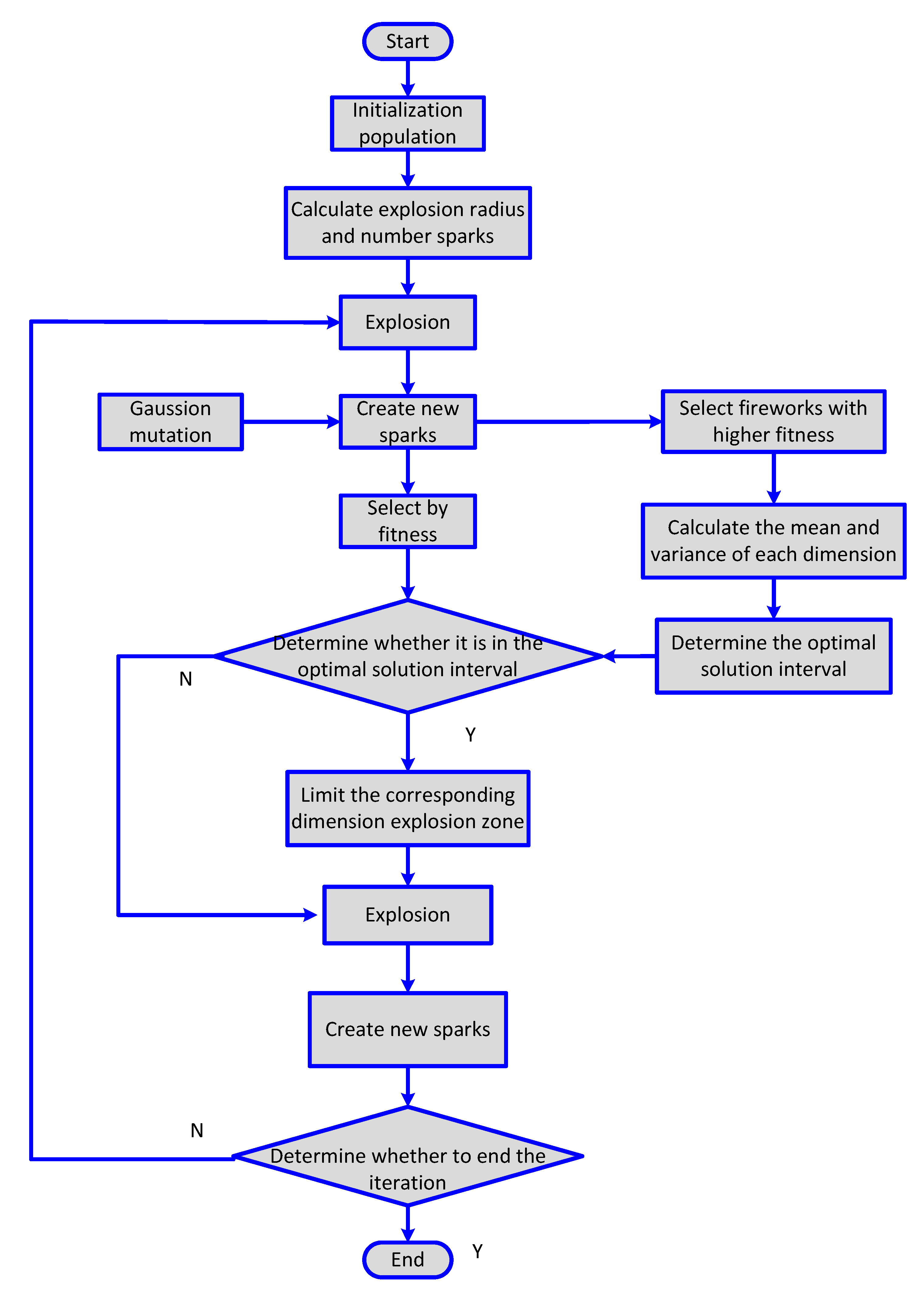
2.1. Fireworks Algorithm and Improved Fireworks Algorithm

The FWA is a new swarm intelligent algorithm, which originates from the phenomenon of fireworks explosion [23]. In the solution process, the firework is treated as a feasible solution of the optimization problem. The process of searching for the neighborhood union of the feasible solution is the fireworks explosion, which generates a certain number of sparks. The local search and global search are accomplished by controlling the number of sparks generated from each fireworks explosion. In the feasible solutions, the fireworks with poor fitness have larger explosion radius, which leads to greater exploration abilities. Conversely, the fireworks with better fitness have smaller explosion radius, which leads to more excavation capacity around the position. The Gaussian mutation is applied to the original sparks for increasing the diversity of the population.

The specific solution steps of FWA are as follows [24,25,26,27,28].

(1) For the optimization problem, the initial fireworks are $N$, which are randomly generated in the feasible solution space $\mathsf{\Omega }$.

(2) The fitness of each firework is evaluated. The radius of each firework $R_i$ and the number $S_i$ of sparks generated from the explosion are calculated. $R_i$ and $S_i$ are expressed as follows.

$$R_i=R_c\times \frac{f(x_i)-y_{\min }+\epsilon }{{\displaystyle \sum _{i=1}^N(f(x_i)-y_{\min })+\epsilon }}$$

(1)

$$S_i=u\times \frac{y_{\max }-f(x_i)+\epsilon }{{\displaystyle \sum _{i=1}^N(y_{\max }-f(x_i))+\epsilon }}$$

(2)

where $f(x_i)$ is the fitness function of the optimized problem. $y_{\min }$ and $y_{\max }$ are the best and the worst solution of the fitness in the current fireworks population. $R_c$ and $u$ are the constants, which are used to adjust the size of the explosion radius and the number of explosion sparks. $\epsilon$ is the smallest amount for the machine, which is used to avoid zero denominator.

(3) To further seek the optimal solution and avoid the coincidence of the explosion spark position, fireworks with better fitness should explode in a small range. The fireworks with worse fitness should explode in a large range to achieve better global search. Equation (3) is used to limit the number of explosion sparks as follows.

$$S_i=\{\begin{array}{l}\begin{array}{cc}round(a\ast u)& S_i<a\ast u\end{array}\hfill \\ \begin{array}{cc}round(b\ast u)& S_i>b\ast u\&a<b<1\end{array}\hfill \\ \begin{array}{cc}round(S_i)& other\end{array}\hfill \end{array}$$

(3)

where $a$ and $b$ are constants. $round$ is rounding function.

(4) If all sparks are generated from fireworks explosion, the spark population is too simple. Thus, the Gaussian mutation is applied to generate new sparks. The generating process of mutation sparks is as follows. A firework $x_i$ is randomly generated from the fireworks population. A certain number of sparks selected randomly are carried out Gaussian mutation operation. The sparks with $k$ dimensions are chosen from the fireworks $x_i$. Gaussian mutation operation is expressed as follows.

$${\widehat{x}}_{ik}=x_{ik}\times e$$

(4)

where $e~N(1,1)$, $N(1,1)$ is the Gaussian distribution; ${\widehat{x}}_{ik}$ is the -dimensional value of the Gaussian spark; $x_{ik}$ is the $k$ dimensional value of the explosion; and $e$ is generated randomly.

The range of sparks is expanding in the explosion process as the sparks are generated from the fireworks explosion. It is necessary to limit the spark position, because it may go beyond the boundaries of the viable domain $\mathsf{\Omega }$. Equation (5) is used to map the spark $x_i$, which is beyond the dimension.

$${\widehat{x}}_{ik}=x_{LowB,k}+\left|x_i\right|(x_{UpB,k}-x_{LowB,k})$$

(5)

where $x_{UpB,k}$ and $x_{LowB,k}$ are the upper and lower bounds of the solution space on the dimension $k$.

(5) If the new spark generated from the explosion and mutation cannot meet the termination condition, then $N$ sparks are selected from the fireworks. The sparks and the mutation sparks are selected as the fireworks of next generation explosion. The unselected fireworks disappear. This paper assumes the total number of fireworks, explosions sparks, and mutation sparks is $M$. The size of fireworks is $N$. The spark with best fitness should be chosen as the next generation firework. Then, $N-1$ sparks are chosen from the remaining $M-1$ fireworks by using the roulette method. The probability of the candidate sparks chosen as the next explosion fireworks is as follows.

$$p(x_{ik})=\frac{R(x_i)}{{\displaystyle \sum _{x_j\in k}{x}_j}}$$

(6)

where $R(x_i)={\displaystyle \sum _{x_j\in k}d(x_i-x_j)=}{\displaystyle \sum _{x_j\in k}\Vert x_i-x_j\Vert }$.

When the selection strategy is used, the fewer sparks there are around is an individual, the greater the probability that the spark is selected as the next explosion fireworks. The explosion and selection processes are repeated until the termination conditions are met.

The original mapping rules of the FWA algorithm cause the algorithm to converge slowly. In view of the deficiencies of the traditional fireworks algorithm, this paper proposes a new improved fireworks algorithm. The best position is at or near the origin. For the solution that is out of bounds in the FWA, according to the mapping rule of Equation (5), the value of one of the firework positions in one dimension is mapped to a position close to the origin. The optimal solution of optimization problems is at the origin, which can accelerate the convergence process of the algorithm to a certain extent. To avoid the illusion of the premature convergence, a new mapping rule is applied, which is expressed as follows.

$${\widehat{x}}_{ik}=x_{LowB,k}+U(0,1)(x_{UpB,k}-x_{LowB,k})$$

(7)

where $U(0,1)$ represents a random number of uniform distribution on the interval [0,1].

Gaussian mutation is applied to generate new sparks in the FWA to avoid the fireworks population of the explosion being too simple, which is shown in Equation (4). This Gaussian mutation has flaws. For example, when the $e$ is close to 0, the position of the Gaussian mutation fireworks is close to 0. The optimal solutions are close to the origin in optimization problems, which may converge to the optimal point after a small number of iteration times. The traditional Gauss mutation method not only enlarges the diversity of fireworks, but also reduces the convergence speed of the algorithm. To solve this problem, the optimal fireworks explosion position is introduced into the improved fireworks, which makes the fireworks ensure the diversity and accelerate the algorithm convergence speed. A new Gaussian mutation spark ${\widehat{x}}_{ik}$ equation is proposed to solve this problem, which is expressed as follows.

$${\widehat{x}}_{ik}=x_{ik}+(x_{Bk}-x_{ik})\times e$$

(8)

where $e~N(0,1)$; $N(0,1)$ represents a Gaussian distribution whose mean value and variance is 0 and 1. $x_{Bk}$ is the position of the fireworks with the best fitness of the current fireworks population in the $k_{th}$ dimension.

The traditional FWA controls the radius and the number of sparks generated from fireworks explosion using Equations (1) and (2). The better the original fireworks fitness is, the smaller the spark radius is. The poorer the fitness is, the larger the spark radius is. A better solution is obtained by expanding the search scope. The entire fireworks are treated variates during the fireworks explosion. Because of the randomness of the explosion, the dimension change in the fireworks may explode in the direction of deviation from the optimal solution, which may result that the local search cannot be completed. An improved method is proposed to enhance the local search. The specific process is as follows.

(1) Ten sparks with better fitness are chosen. Suppose that each spark $x_i$ is divided into $p$-dimensional variates $c_{i1},c_{i2},\cdots ,c_{ip}$. The mean value ${\overline{c}}_p$ and standard deviation $S_p$ of each dimension variate are calculated. The equations are expressed as follows.

$${\overline{c}}_p={\displaystyle \sum _{i=1}^{10}{c}_{ip}/10}$$

(9)

$$S_p=\sqrt{{\displaystyle \sum _{i=1}^{10}{(c_{ip}-{\overline{c}}_p)}^2/10}}$$

(10)

If the standard deviation of one demission variate in the spark is small, the variate with better fitness is more concentrated. The spark should be strengthened searching in the vicinity of the mean value. Conversely, if the standard deviation of one demission variate in the spark is large, the optimal solution position cannot be determined. Thus, the radius of the explosion should be expanded to complete the global search. The $q$-dimensional variate is chosen from $p$-dimensional variate with better fitness to enhance local search by comparing the standard deviation of each dimension variate.

(2) The best fitness spark is chosen from the first explosion sparks, mutation sparks, and the original fireworks. Then, remaining sparks are selected randomly. Before the fireworks explosion, the $q$-dimensional variate is screened to determine whether a dimension variate is in the interval $[{\overline{c}}_p-S_p,{\overline{c}}_p+S_p]$. If the dimension variate is in the interval, this dimension variate is in the optimal solution range. The next explosion range is defined in the interval $[{\overline{c}}_i-S_i,{\overline{c}}_i+S_i]$, which can strength local search ability. For variates that are out of $[{\overline{c}}_p-S_p,{\overline{c}}_p+S_p]$ and unselected $p-q$ dimension variates are exploded by the original way.

(3) Ten sparks with better fitness are chosen. Steps (1) and (2) are repeated.

(4) Judge whether the results satisfy the termination condition. If the condition is not satisfied, the explosion and selection steps are repeated until the condition is satisfied.

The main steps of IFWA are as follows

(1)

The parameters of IFWA are initialized: the number of fireworks, the number of variant sparks, the maximum number of iterations, etc.

(2)

The number of sparks and the radius of fireworks explosion are calculated.

(3)

The sparks explode, their position is obtained, and the fitness value of sparks is calculated.

(4)

The Gauss variation sparks are generated and the fitness value of Gauss sparks is calculated.

(5)

The sparks satisfying the conditions are limited to the explosion range and the sparks that do not satisfy the conditions are exploded in the original way.

(6)

If the termination condition is not satisfied, go to Step 2. if the result is satisfied, the iteration is terminated.

The flow chart of the IFWA is shown in Figure 1.

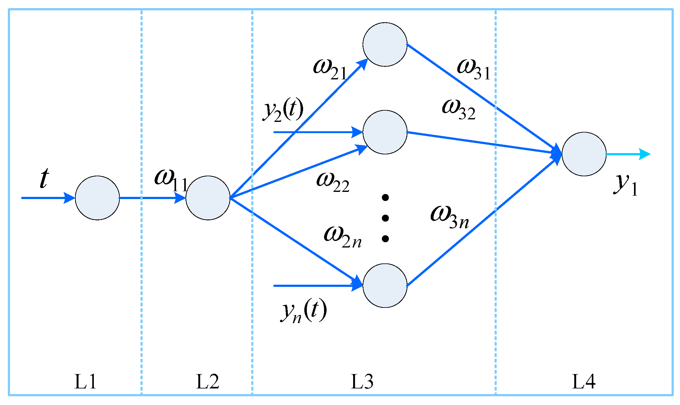
2.2. Multi-dimensional Grey Model and Grey Neural Network Model

Grey model (GM) is to set up grey differential equations through a small amount of discontinuous information. The basic idea of grey model is to use the original data to form the original sequence, which can weaken the randomness of the original data and reflect the continuous change process of internal things. The multi-dimensional grey dynamic prediction model is GM ($1$,$n$) model, which is order 1 and $n$ represents independent variables. The modeling process of GM ($1$,$n$) model is as follows [5].

Suppose that the original sequence has $n$ variates and each variate corresponds to the sequence of $m$ datasets [29,30].

$$\left\{x_i^{(0)}(k)\right\}(k=1,2,\cdots ,m;i=1,2,\cdots ,n)$$

(11)

The original sequence $x_i^{(0)}(k)$ is accumulated to obtain a new data sequence $x_i^{(1)}(k)$.

$$x_i^{(1)}(k)={\displaystyle \sum _{j=1}^k{x}_i^{(0)}}(j)$$

(12)

The mean value generation sequence with consecutive neighbors of $x_1^{(1)}(k)$ is $z_1^{(1)}(k)$.

$$z_1^{(1)}(k)=0.5\ast x_1^{(1)}(k)+0.5\ast x_1^{(1)}(k-1)\hspace{1em}k=2,3,\cdots ,n$$

(13)

The data matrix $B$ and the vector matrix $y_n$ is expressed as follows.

$$\begin{array}{l}B=\left[\begin{array}{cccc}-z_1^{(1)}(2)& x_2^{(1)}(2)& \cdots & x_n^{(1)}(2)\\ -z_1^{(1)}(3)& x_2^{(1)}(3)& \cdots & x_n^{(1)}(3)\\ ⋮& ⋮& ⋮& ⋮\\ -z_1^{(1)}(m)& x_2^{(1)}(m)& \cdots & x_n^{(1)}(m)\end{array}\right]\\ y_n={\left[\begin{array}{cccc}{x}_1^{(0)}(2),& x_1^{(0)}(3),& \cdots ,& x_1^{(0)}(m)\end{array}\right]}^T\end{array}$$

(14)

The parameter identification array $p_n$ is expressed as follows.

$$p_n=\left[\begin{array}{c}a\\ b_2\\ b_3\\ ⋮\\ b_n\end{array}\right]={(B^{T}B)}^{-1}{B}^T{y}_n$$

(15)

The predictive model is expressed as follows.

$${\widehat{x}}^{(0)}(k)={\displaystyle \sum _{i=2}^m{b}_i{x}_i^{(1)}(k)}-a{z}_1^{(1)}(k)$$

(16)

The relative error of the model is expressed as follows.

$$e(k)=\frac{\left|{\widehat{x}}_1^{(0)}(k)-x_1^{(0)}(k)\right|}{x_1^{(0)}(k)}\ast 100$$

(17)

The characters of grey model (GM) are small sample size and simple model structure. However, the self-learning ability of the grey prediction model is insufficient. The processing capacity of GM is relatively weak for more complex nonlinear systems [6]. Back propagation neural network has high mapping ability for the nonlinear function and can approximate any functions with any accuracy. The prediction accuracy is improved by combining the lower data modeling of the grey system theory with the nonlinear mapping of the neural network. The modeling process of grey neural network (GNN) is as follows [9].

The original sequence $x_t^{(0)}$ is expressed as $x(t)$. $x(t)$ is accumulated to obtain a new data sequence $x_t^{(1)}$. $x_t^{(1)}$ is expressed as $y(t)$ and the prediction result $x_t^{\ast (1)}$ is expressed as $z(t)$.

The differential equation of the GNN model with $n$ parameters are expressed as follows.

$$\frac{d{y}_1}{dt}+a{y}_1=b_1{y}_2+b_2{y}_3+\cdots +b_{n-1}{y}_n$$

(18)

where $y_2,\cdots ,y_n$ are the input parameters of the system; $y_1$ is the output parameter of the system; and $a,b_1,b_2,\cdots ,b_{n-1}$ are the coefficients of differential equations.

The time response of Equation (7) is expressed as follows.

$$\begin{array}{ll}z(t)=& \left[y_1(0)-\frac{b_1}{a}{y}_2(t)-\frac{b_2}{a}{y}_3(t)-\cdots -\frac{b_{n-1}}{a}{y}_n(t)\right]e^{-at}+\frac{b_1}{a}{y}_2(t)\\ & +\frac{b_2}{a}{y}_3(t)+\cdots +\frac{b_{n-1}}{a}{y}_n(t)\end{array}$$

(19)

Suppose $d=\frac{b_1}{a}{y}_2(t)+\frac{b_2}{a}{y}_3(t)+\cdots +\frac{b_{n-1}}{a}{y}_n(t)$ and Equation (19) is transformed as follows.

$$\begin{array}{ll}z(t)& =\left[(y_1(0)-d)\ast \frac{e^{-at}}{1+e^{-at}}+d\ast \frac{1}{1+e^{-at}}\right]\ast (1+e^{-at})\\ & =\left[(y_1(0)-d)\ast (1-\frac{e^{-at}}{1+e^{-at}})+d\ast \frac{1}{1+e^{-at}}\right]\ast (1+e^{-at})\\ & =\left[(y_1(0)-d)-y_1(0)\ast \frac{e^{-at}}{1+e^{-at}}+2d\ast \frac{1}{1+e^{-at}}\right]\ast (1+e^{-at})\end{array}$$

(20)

After transformation, Equation (20) is mapped to an extended back propagation neural network. The GNN model with $n$ input parameters and 1 output parameter is established. The topology is shown in Figure 2.

In Figure 2, $t$ is the input parameter for the network; n is the number of neurons in the third layer; $y_2(t),\cdots ,y_n(t)$ are the output parameters of the network; ${\omega }_{21},{\omega }_{22},\cdots ,{\omega }_{2n},{\omega }_{31},{\omega }_{32},\cdots ,{\omega }_{3n}$ are network weights; and $y_1$ is the network prediction value [23,24].

Set $\frac{2b_1}{a}=u_1,\frac{2b_2}{a}=u_2,\cdots ,\frac{2b_{n-1}}{a}=u_{n-1}$. The initial network weights are expressed as follows.

$$\begin{array}{l}{\omega }_{11}=a\\ {\omega }_{21}=-y_1(0),{\omega }_{22}=u_1,{\omega }_{23}=u_2,\cdots ,{\omega }_{2n}=u_{n-1}\\ {\omega }_{31}={\omega }_{32}=\cdots ={\omega }_{3n}=1+e^{-at}\end{array}$$

The threshold of the output node of the L4 layer is expressed as follows.

$$\theta =(1+e^{-at})(d-y_1(0))$$

(21)

In this paper, the number of L3 neurons is determined according to Equation (22).

$$L{3}_n=\sqrt{({input}_n+{output}_n)}$$

(22)

where ${input}_n$ is the number of model input variables. ${output}_n$ is the number of output variables.

2.3. Improved Fireworks Algorithm Optimization Grey Neural Network

The weights and thresholds of GNN are determined randomly. If the weights and thresholds are not selected properly, the GNN model easily falls into local optimum. The six variates $a,b_1,b_2,b_3,b_4,b_5$ of GNN model need to be optimized. The prediction effect of GNN model is improved by optimizing the parameters of GNN model. This study uses IFWA to optimize GNN parameters and establish the IFWA-GNN model. The modeling process of IFWA-GNN model for relay life prediction is as follows.

(1)

The input and output parameters of the predictive model are determined.

(2)

The input and output of the model are normalized.

(3)

The basic parameters of the fireworks algorithm are initialized: the maximum number of iterations, the number of fireworks, etc.

(4)

The IFWA is used to optimize the parameters of GNN model.

(5)

The optimized parameters are entered into the GNN model.

(6)

The IFWA-GNN model is used to predict the life of relay, and the predicted results are inversely normalized.

(7)

The evaluation indicators are used to evaluate the prediction model.

3. The Relay Experiment and Parameters Analysis

3.1. The Relay Experiment

When the relay is energized, the contacts are closed. The mechanical collision of dynamic and static contacts causes the vibration and bounce of the contacts, which indicates that the stable state of the contacts cannot be reached immediately. The contacts have a process of bounce. The dynamic contact and static contact have different dynamic contact characteristics. There are faults in electromagnetic relay and different kinds of failure mode. However, the failures caused by contact of relay account for more than 80% of relay failures.

Thirteen HH52P small relays (Shanghai People Electric Co., Ltd, Shanghai, China) were used for life test. The performance parameters of the relay are shown in

Table 1. HH52P type relay parameters.

Model	HH52P
Contact rating	5A
Contact form	2H, 2D, 2Z
Coil power	0.9W
Contact resistance	$\le 50m\mathsf{\Omega }$
Insulation resistance	$\ge 100M\mathsf{\Omega }$
Contact material	Silver alloy

. The relays are divided into three groups to simulate the actual working conditions due to the certain difference in the working environment of the relay. The reliability tests are carried out at temperatures of -20, 20, and 55 °C in the incubator. A constant current of 5 A is applied to the relay to obtain a large dynamic contact voltage drop peak and a static contact pressure drop since the contact resistance between the contacts is small and difficult to measure.

The bounce time of the contact, the duration of the dynamic contact resistance, the peak of the dynamic contact pressure drop, and the static contact pressure drop are tested. The measurement is performed every same time and the values of each parameter at different temperatures are recorded separately. The number of intermediate intervals is set to 10,000 times. If the measured values differ more or are unstable in a certain period, the number of measurements is appropriately increased. The test interval should be shortened and the number of test groups increased at the beginning of life since the relay life prediction is based on its vital state information. The life of the relay used in the test is generally about one million times. The test data of the first 10,000 times are used as the basis for judging the initial state of life.

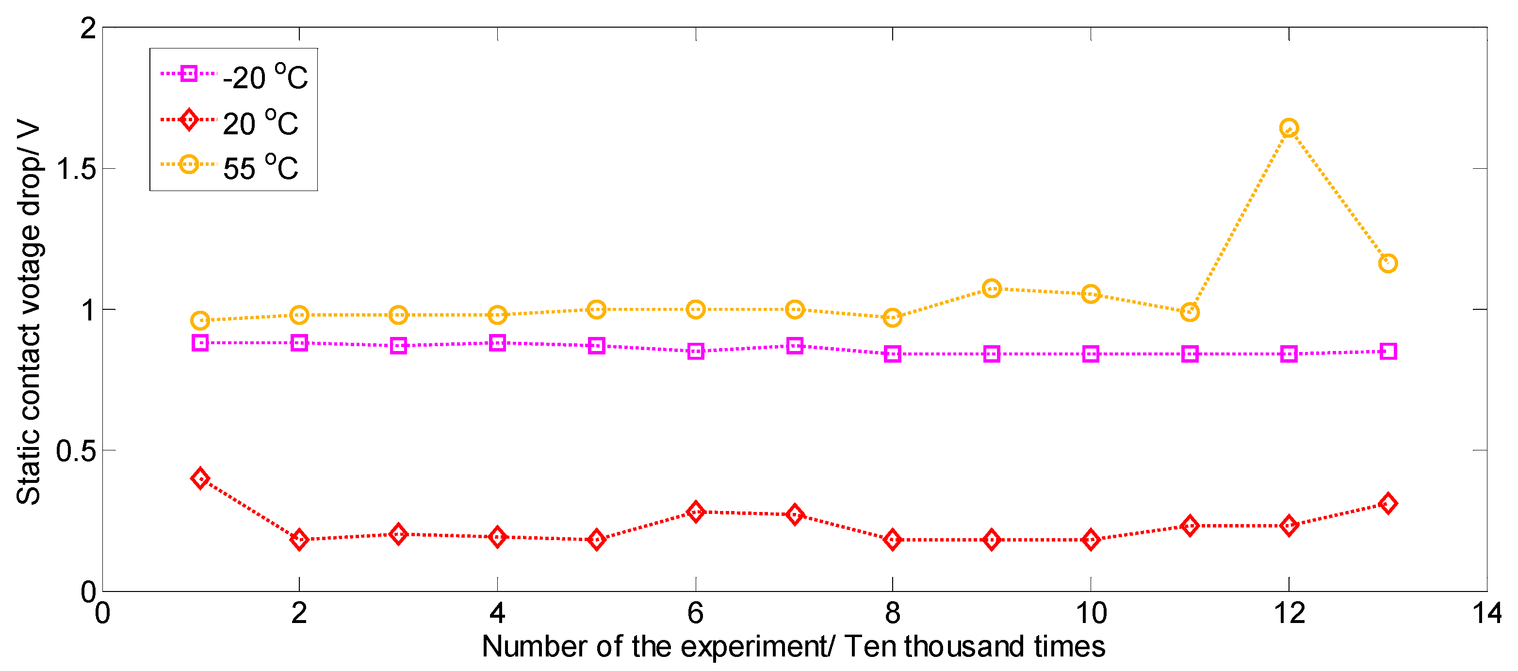
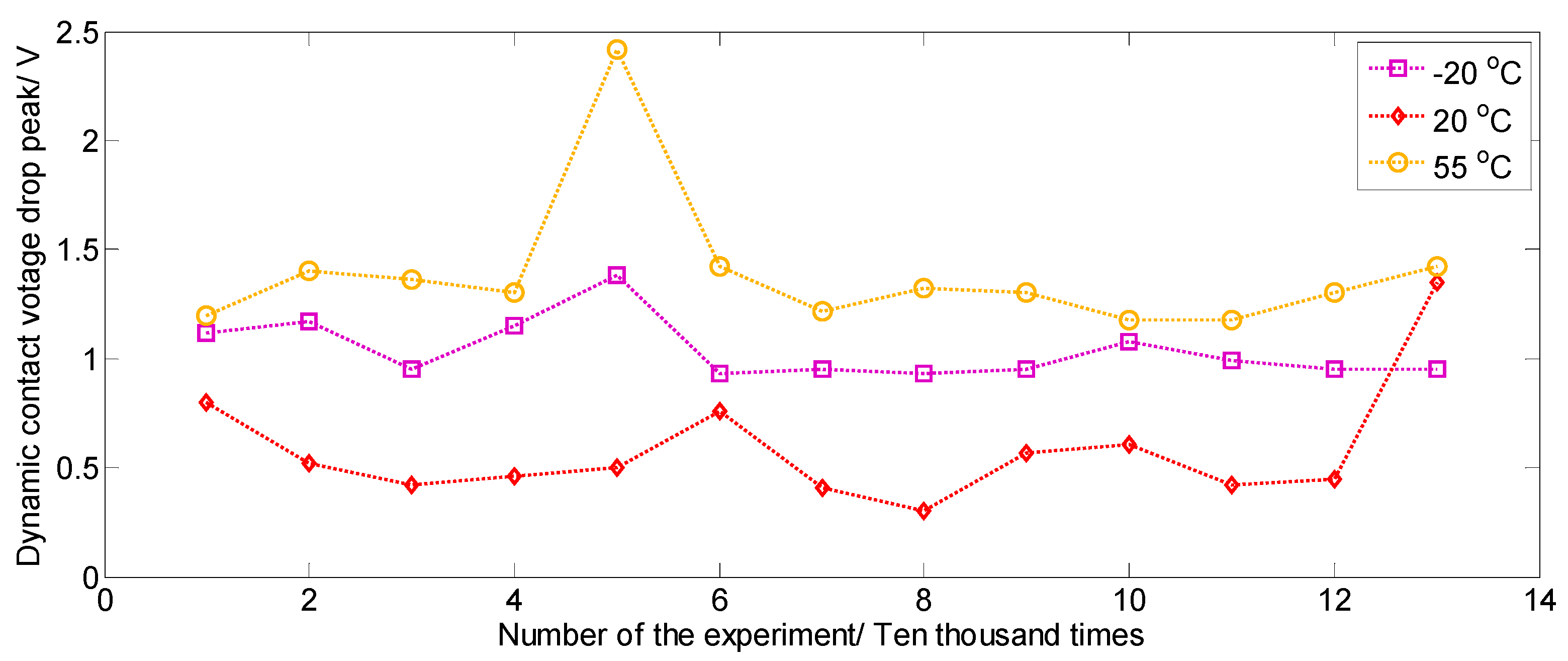
3.2. Parameter Analysis

Parameters describe the performance of a relay contact. The bounce time and contact resistance are commonly used. The bounce time includes the bounce time of the contact and the steady time of the contact in the dynamic process of closure. The contact causes grain fatigue on the contact surface and mechanical wear. The bounce time is changed by the wear of contact surface, thus the condition of contact wear is reflected by the bounce time.

In the applied process of the relay, the contact resistance value also changes constantly owing to the phenomena of oxidation, electrochemical reaction, and wear. The contact failure occurs when the contact resistance value exceeds the limit. The dynamic contact resistance and static contact resistance are two important parameters of the performance of relay. However, it is not easy to measure the contact resistance directly. The contact resistance is expressed by measuring the contact voltage drop indirectly. The contact voltage drop is also divided into the dynamic contact voltage drop and static contact voltage drop. The dynamic contact voltage drop is the voltage drop from just touching the steady state of the intermediate process, which is always reflected by the dynamic contact voltage drop peak. The static contact voltage drop is the voltage drop after steady contact.

The working environment of relay is complicated. The reliability of relay is related to the external environment. Temperature is an important parameter. High temperature causes the coil resistance to increase and accelerate the deformation of the insulating material. If the sealing is poor, the low temperature leads to the formation of frost between the contacts. Thus, temperature is a parameter that must be considered in the lifetime experiment of relay.

The HH52P relay is taken as an example. The four parameters are taken as the measuring indexes which contain contact bounce time $t_{\mathrm{T}}$, duration of dynamic contact resistance $t_{\mathrm{D}}$, dynamic contact voltage drop peak, and static contact voltage drop $V_{\mathrm{C}}$. Thirteen groups relay are taken to conduct lifetime experiment at −20 °C, 20 °C and 55 °C. The experimental results are shown in

Table 2. Experimental results of relay at −20 °C.

Temperature (°C)	Times (Ten Thousands Times)	${\mathit{t}}_{\mathit{T}}\left(\mathbf{ms}\right)$	${\mathit{t}}_{\mathit{D}}\left(\mathbf{ms}\right)$	${\mathit{V}}_{\mathit{m}}\left(\mathbf{V}\right)$	${\mathit{V}}_{\mathit{C}}\left(\mathbf{V}\right)$
−20	10	0.71	0.20	1.12	0.88
−20	50	0.44	0.69	1.17	0.88
−20	100	1.49	0.22	0.95	0.87
−20	150	0.91	0.62	1.15	0.88
−20	200	0.57	0.69	1.38	0.87
−20	250	0.50	0.76	0.93	0.85
−20	300	0.51	1.39	0.95	0.87
−20	350	1.06	0.75	0.93	0.84
−20	400	0.69	1.28	0.95	0.84
−20	450	0.54	1.08	1.08	0.84
−20	500	0.49	1.12	0.99	0.84
−20	550	0.69	1.28	0.95	0.84
−20	600	0.82	0.67	0.95	0.85

,

Table 3. Experimental results of relay at 20 °C.

Temperature (°C)	Times (Ten Thousands Times)	${\mathit{t}}_{\mathit{T}}\left(\mathbf{ms}\right)$	${\mathit{t}}_{\mathit{D}}\left(\mathbf{ms}\right)$	${\mathit{V}}_{\mathit{m}}\left(\mathbf{V}\right)$	${\mathit{V}}_{\mathit{C}}\left(\mathbf{V}\right)$
20	10	1.01	0.88	0.80	0.4
20	50	0.35	1.24	0.52	0.18
20	100	0.42	0.60	0.42	0.20
20	150	0.43	0.94	0.46	0.19
20	200	0.41	0.65	0.50	0.18
20	250	0.55	1.96	0.76	0.28
20	300	0.82	0.55	0.41	0.27
20	350	0.78	0.57	0.30	0.18
20	400	0.42	0.76	0.57	0.18
20	450	0.76	0.31	0.61	0.18
20	500	0.85	3.34	0.42	0.23
20	550	0.81	1.29	0.45	0.23
20	600	0.88	2.00	1.35	0.31

and

Table 4. Experimental results of relay at 55 °C.

Temperature (°C)	Times (Ten Thousands Times)	${\mathit{t}}_{\mathit{T}}\left(\mathbf{ms}\right)$	${\mathit{t}}_{\mathit{D}}\left(\mathbf{ms}\right)$	${\mathit{V}}_{\mathit{m}}\left(\mathbf{V}\right)$	${\mathit{V}}_{\mathit{C}}\left(\mathbf{V}\right)$
55	10	0.34	0.86	1.20	0.96
55	50	0.53	0.55	1.40	0.98
55	100	0.55	0.23	1.36	0.98
55	150	0.49	0.32	1.30	0.98
55	200	1.54	0.65	2.42	1.00
55	250	0.41	0.42	1.42	1.00
55	300	0.49	0.26	1.22	1.00
55	350	0.57	2.38	1.32	0.97
55	400	0.46	1.38	1.30	1.07
55	450	0.36	1.39	1.18	1.05
55	500	0.36	0.69	1.18	0.99
55	550	0.46	1.38	1.30	1.64
55	600	0.36	0.62	1.42	1.16

.

The static contact voltage drop and the dynamic contact voltage drop peak are taken as examples, which can reflect the change law of different parameters with the increase of the number of lifetime experiment at different temperatures. The line graphs are as follows.

There are some sharp points from the experimental data in Figure 3 and Figure 4, which are due to the influence of the experimental environment and the material itself. To imitate the operating state of the relay under real conditions, these sharp points are retained in this paper. Figure 3 and Figure 4 show that the static contact voltage drop of each relay at different temperatures is different. The static contact voltage drop at 20 °C is smaller than that at −20 °C and 55 °C. The static contact voltage drop at 20 °C is about 0.15–0.3 V, while the voltage drop is about 0.8–0.9 V at −20 °C and the voltage drop is about 0.9–1.1 V at 55 °C. The static contact voltage drop fluctuates greatly at 20 °C. The dynamic contact voltage drop is different at different temperatures. The dynamic contact voltage drop peak at 20 °C is lower than that at −20 °C and 55 °C. The performance of relay is different at different temperatures. Hence, the temperature should be taken into account when the performance parameters of relay are used to predict the lifetime.

4. Experiment Results

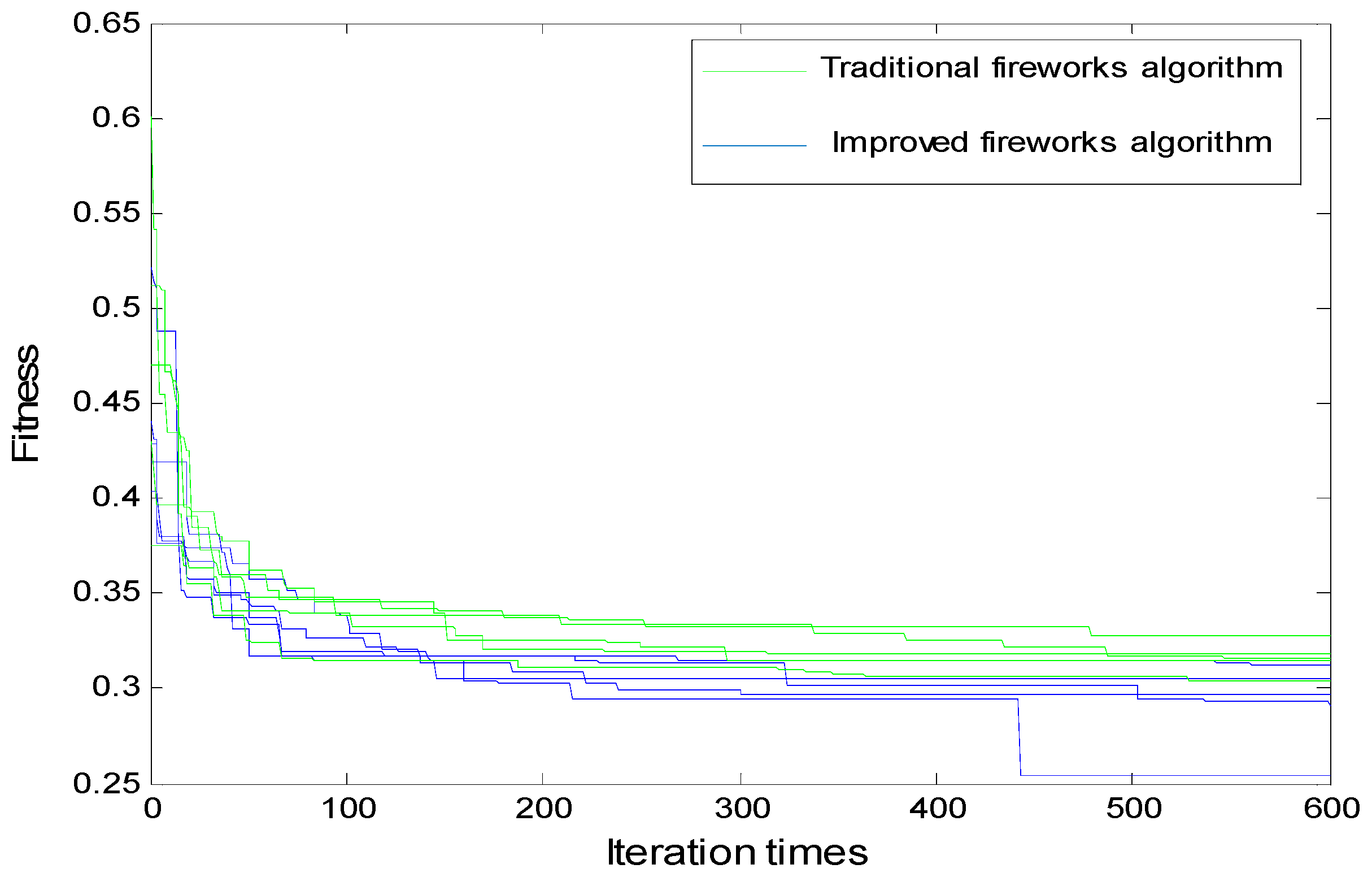
4.1. IFWA Performance Analysis

Three standard test functions are used to analyze the IFWA convergence performance and compare it with FWA. The standard test functions are shown in

Table 5. Test function.

Test Function	Optimal Value	Range of Values
	0	[−100, 100]
$Y_2={\displaystyle \sum _{i=1}^m\left|s_i\right|}+{\displaystyle \prod _{i=1}^m\left|s_i\right|}$	0	[−10, 10]
$Y_3={\displaystyle \sum _{i=1}^m(s_i^2-10\ast \cos (2\pi \ast s_i+10))}$	0	[−5.12, 5.12]

[31,32].

The parameter settings of FWA and IFWAs are shown in

Table 6. Parameter setting.

Algorithm	Parameters
FWA	Itera = 2000, D = 100, SeedN = 5, SonN = 50, MutaN = 5, Amp = 0.5, SparksmaxN = 40, SparksminN = 2
IFWA	Itera = 2000, D = 100, SeedN = 5, SonN = 50, MutaN = 5, Amp = 0.5, SparksmaxN = 40, SparksminN = 2

.

Table 6 presents that the maximum number of iterations is set to 2000 and the test dimension is 100. Seed_N is the number of fireworks. Son_N is the number of sparks. Muta_N is the number of variant sparks.

The three optimization algorithms are tested repeatedly for 15 times using three standard test functions. The test results are shown in

Table 7. Test results.

Y	Algorithm	Optimal Value	The Worst Value	Average Value	Average Running Time of Program (s)
Y1	FWA	4.51 × 10−21	2.88 × 10−6	2.11 × 10−7	1.14
	IFWA	2.20 × 10−32	8.59 × 10−25	5.81 × 10−26	0.86
Y2	FWA	7.79 × 10−10	1.51 × 10−5	4.21 × 10−6	0.98
	IFWA	1.74 × 10−16	1.69 × 10−13	2.07 × 10−14	0.77
Y3	FWA	1.77 × 10−15	5 × 10−2	3.8 × 10−3	1.01
	IFWA	0	0	0	0.88

.

Table 7 presents the optimal values of the three standard test functions are all 0. It is found that the optimal convergence, the worst convergence, and the average convergence of the IFWA in Table 7 are the closest to 0. The 15 tests of IFWA for function Y₃ converge to the optimal value of 0. Compared with the traditional FWA, the convergence accuracy of IFWA has been obviously improved. The average running time of IFWA is the shortest after 15 repeated tests of the three algorithms. Through comparison, the results show that the convergence accuracy and running speed of IFWA are improved compared with FWA.

4.2. Simulation Test Data and Evaluation Index

The relay lifetime prediction is based on multi-dimensional GM, GNN model, FWA-GNN model, and the IFWA-GNN model. The corresponding performance parameters and the final lifetime of each relay are recorded at different temperatures. The GM, GNN, FWA-GNN, and IFWA-GNN models were trained with the data in Table 2, Table 3 and Table 4. The four models were tested with the data in

Table 8. The initial performance parameters of relay and its lifetime.

Lifetime (Ten Thousands Times)	Temperature (°C)	${\mathit{t}}_{\mathit{T}}\left(\mathbf{ms}\right)$	${\mathit{t}}_{\mathit{D}}\left(\mathbf{ms}\right)$	${\mathit{V}}_{\mathit{m}}\left(\mathbf{V}\right)$	${\mathit{V}}_{\mathit{C}}\left(\mathbf{V}\right)$
612	−20	0.54	0.63	0.67	0.90
693	−20	0.71	0.20	0.91	0.88
752	−20	0.43	0.69	1.12	0.88
788	−20	0.92	0.69	1.61	0.88
900	−20	1.89	0.69	2.58	0.91
689	20	0.95	0.20	1.15	0.04
711	20	0.71	0.48	1.19	0.13
755	20	0.55	0.84	1.39	0.18
807	20	1.01	0.88	1.89	0.40
834	20	0.73	1.30	2.03	0.22
807	55	0.50	0.25	0.75	1.02
827	55	0.40	0.62	1.02	1.02
837	55	0.34	0.86	1.20	0.96
913	55	0.36	1.39	1.75	1.05
919	55	0.59	1.29	1.88	1.00

.

The average deviation (AD) and root mean square error (RMSE) are used as the evaluation index of model prediction error. The decision coefficient (R2) is used as the evaluation index of model fitting effect.

$$AD=({\displaystyle \sum _{j=1}^m\left|v_j-v_j^{\ast }\right|})/m$$

(23)

$$RMSE=\sqrt{\left({\displaystyle \sum _{j=1}^m{(v_j-v_j^{\ast })}^2}\right)/m}$$

(24)

$$R2=\frac{{(m{\displaystyle \sum v{v}^{\ast }}-{\displaystyle \sum v}{\displaystyle \sum v^{\ast }})}^2}{(m{\displaystyle \sum (v^{\ast }{)}^2}-{\displaystyle \sum (v^{\ast }{)}^2})(m{\displaystyle \sum (v{)}^2}-{\displaystyle \sum (v{)}^2})}$$

(25)

where m is the number of samples; v is the actual value of the sample; and v* is the prediction value of the sample. The range of decision coefficient R2 is between 0 and 1. When the decision coefficient R2 is closer to 1, the input and output of the model are better fitted.

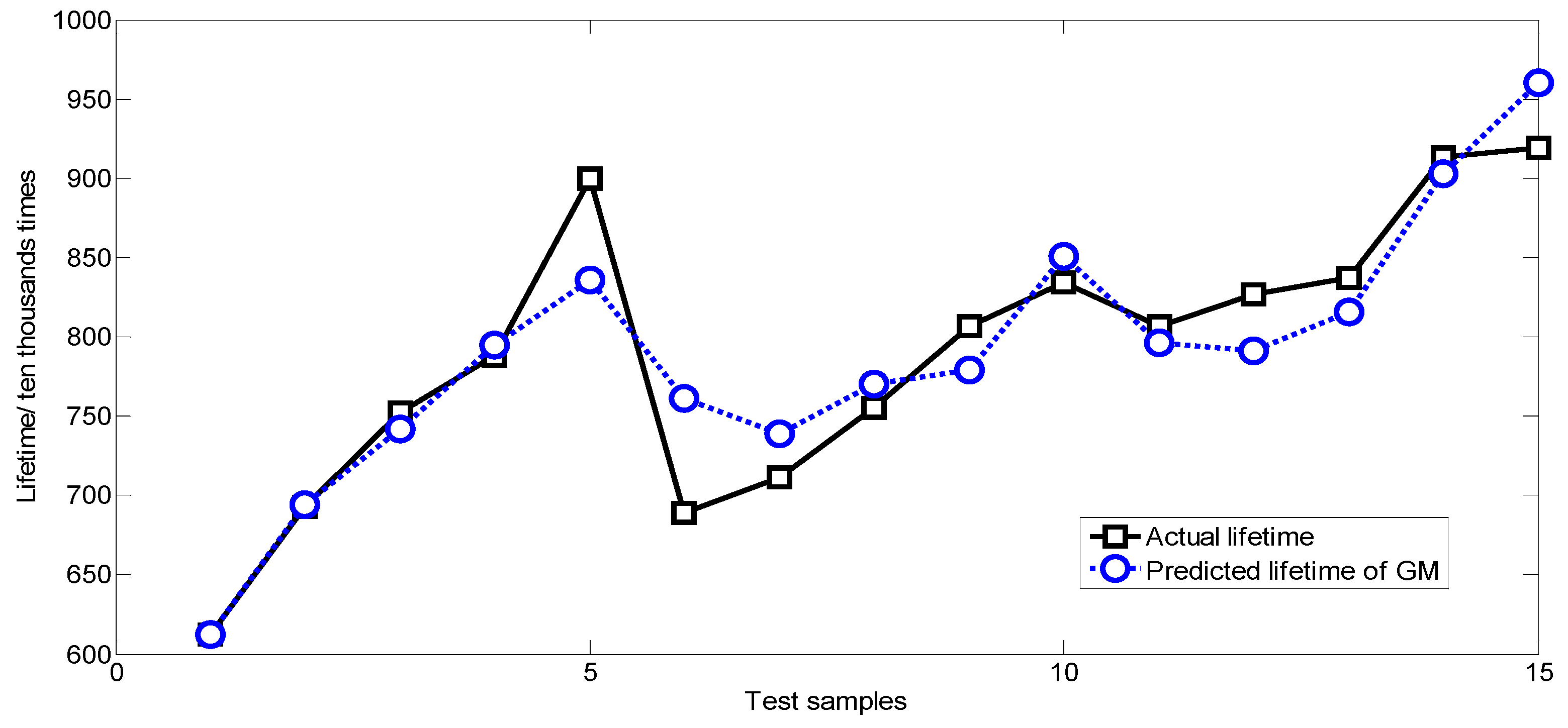
4.3. The Relay Lifetime Prediction Based on Multi-Dimensional GM

The GM (1, 5) model is established to predict relay life. The GM (1, 5) model includes the parameters of the final lifetime, the temperature, the dynamic contact voltage drop peak, the static contact voltage drop, the duration of the dynamic contact resistance, and the contact bounce time. Among them, the final lifetime is the dependent variate and others are the independent variates.

The original data are transformed to eliminate the errors caused by different magnitude between the variates. The transformation equation is expressed as follows:

$$x^{\prime }(k)=x(k)/x(1)$$

(26)

The parameter identification array $p_n$ of the GM is obtained by calculation:

$$p_n={[0.01290.03871.00171.3569-1.31720.0383]}^T$$

(27)

The final prediction equation is expressed as follows:

$$\begin{array}{ll}{\widehat{x}}_1^{(0)}(k)=& 0.0387x_2^{(1)}(k)+1.0017x_3^{(1)}(k)+1.3569x_4^{(1)}(k)\\ & -1.3172x_5^{(1)}(k)+0.0383x_6^{(1)}(k)-0.0129z_1^{(1)}(k)\end{array}$$

(28)

The prediction result of GM (1, 5) model is shown in Figure 5.

Figure 5 indicates the average error between the prediction value and the actual value of each relay is $\overline{e}={\displaystyle \sum _{i=1}^{15}e(i)=3.01\%}$. In sum, the lifetime value predicted by the multi-dimensional GM and the actual relay lifetime still has a larger error.

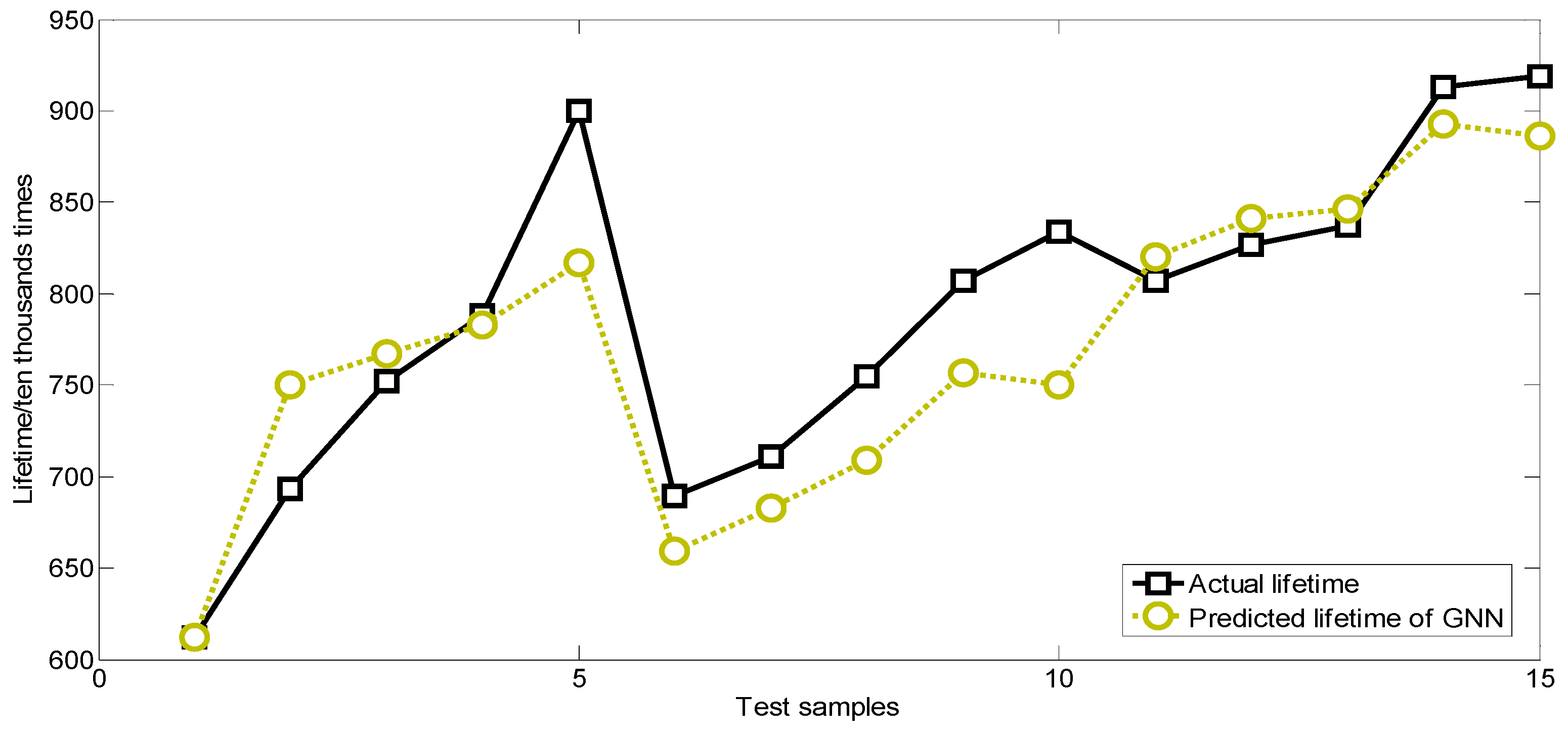
4.4. The Relay Lifetime Prediction Based on GNN Model

The relay lifetime experiment is long, so the number of samples is small. The relay lifetime belongs to the case of fewer data and poor information. Thus, the relay lifetime on the initial state is predicted with the GNN model. The process is as follows.

The original data are accumulated as network input and output parameters. The final output is lifetime and the input variates are the remaining five parameters.

The network parameters and the value of the parameters are initialized. $a,b_1,b_2,b_3,b_4,b_5$ is $0.3+rand(1)/4$.

Learning rate is set to $u_1=u_2=u_3=u_4=u_5=0.0015$.

The weights $\omega$ are calculated according to the definition of the network.

The output of each layer is calculated based on each input sequence $(t,y(t))t=1,2,\cdots ,n$.

L1 layer: $a={\omega }_{11}t$

L2 layer: $b=f({\omega }_{11}t)=\frac{1}{1+e^{-{\omega }_{11}}}$

L3 layer: $c_1=b{\omega }_{21},c_2=y_2(t){\omega }_{22},c_3=y_3(t){\omega }_{23},\cdots ,c_n=y_n(t){\omega }_{2n}$

L4 layer: $d={\omega }_{31}{c}_1+{\omega }_{32}{c}_2+\cdots +{\omega }_{3n}{c}_n-{\theta }_{y1}$

Then, the weights and thresholds are adjusted according to the error between the prediction value of the network output and the expected output.

Error of L4 layer: $\delta =d-y_1(t)$

Error of L3 layer: ${\delta }_1=\delta (1+e^{-{\omega }_{11}t}),{\delta }_2=\delta (1+e^{-{\omega }_{11}t}),\cdots ,{\delta }_n=\delta (1+e^{-{\omega }_{11}t})$

Error of L2 layer: ${\delta }_{n+1}=\frac{1}{1+e^{-{\omega }_{11}t}}(1-\frac{1}{1+e^{-{\omega }_{11}t}})({\omega }_{21}{\delta }_1+{\omega }_{22}{\delta }_2+\cdots +{\omega }_{2n}{\delta }_n)$

Adjust the connection weights of L2 layer to L3 layer:

${\omega }_{21}=-y_1(0),{\omega }_{22}={\omega }_{22}-{\mu }_1{\delta }_{2}b,\cdots ,{\omega }_{2n}={\omega }_{2n}-{\mu }_{n-1}{\delta }_{n}b$

Adjust the connection weights of L1 layer to L2 layer:

${\omega }_{11}={\omega }_{11}+at{\delta }_{n+1}$

Adjust threshold: $\theta =(1+e^{-{\omega }_{11}t})(\frac{{\omega }_{22}}{2}{y}_2(t)+\frac{{\omega }_{23}}{2}{y}_3(t)+\cdots +\frac{{\omega }_{2n}}{2}{y}_n(t)-y_1(0))$.

The prediction result of GNN model is shown in Figure 6.

The trend of training error decreasing with the increasing of evolution time is shown in Figure 7.

Figure 7 presents the convergence rate of the GNN model is fast and the error converges to the minimum at the 12th time. However, this study presents that the prediction results are not ideal. The prediction accuracy is lower than the multi-dimensional GM because the initial parameters of the GNN model are randomly generated and the premature convergence causes the network to jump into the local optimal solution. The GNN parameters are not optimal. The GNN parameters should be optimized to improve the prediction effect of GNN model.

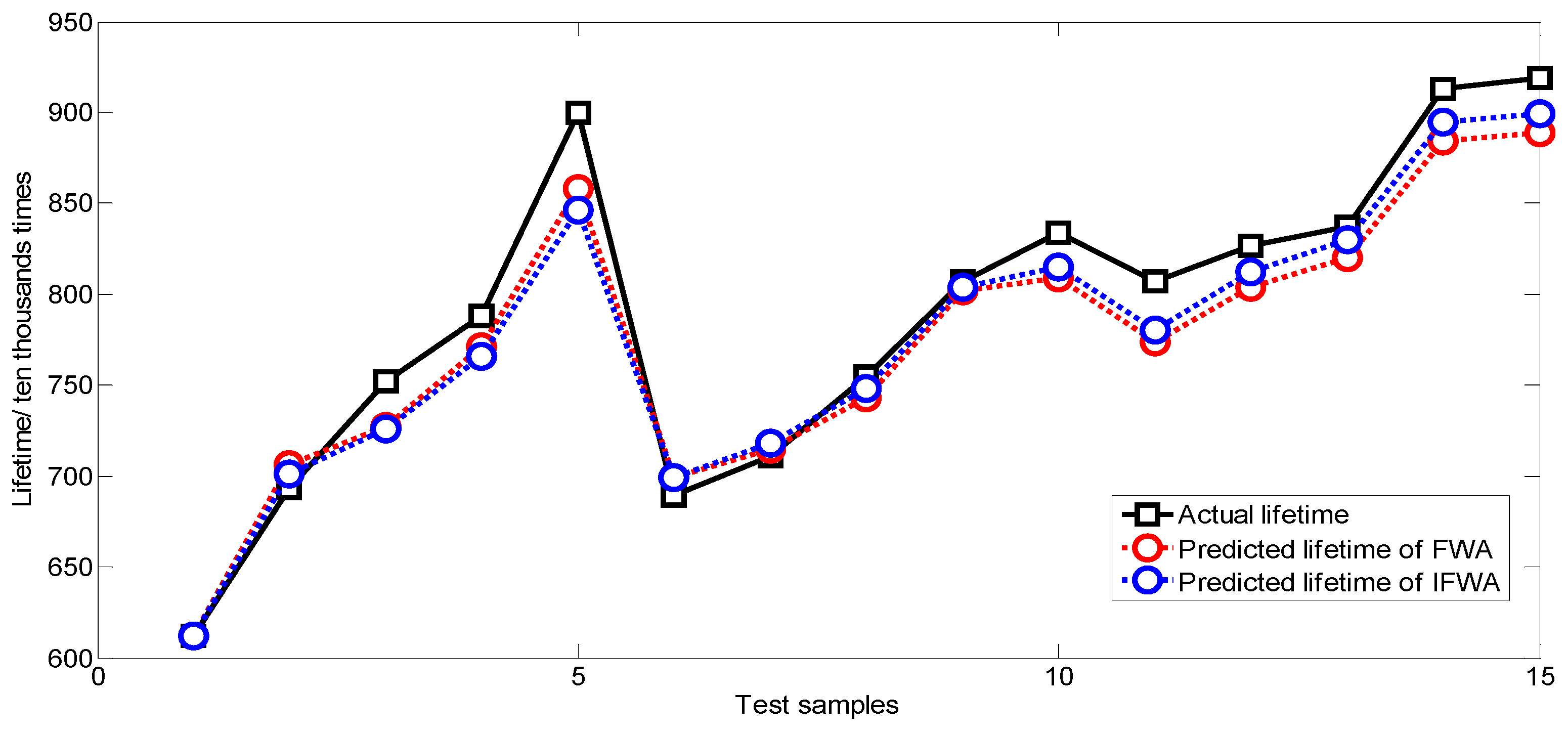
4.5. The Relay Lifetime Prediction Based on the IFWA Optimizing GNN Model

The six variates $a,b_1,b_2,b_3,b_4,b_5$ compose a whole firework and five seed fireworks are randomly generated. The number of each next generation seed fireworks is 5; the maximum number of sparks generated by each seed fireworks explosion is 50; the minimum is 10; the coefficient $u$ of the explosion sparks number $S_i$ is 160; the coefficient $R_c$ of the explosion radius $R_i$ is 0.5; the number of iteration is 600; and the sparks generated by Gaussian mutation is 5.

Ten sparks with better fitness are selected from the sparks generated from the initial fireworks explosion, Gaussian mutation sparks, and the original sparks. The mean value and standard deviation of each dimension variate are calculated. The two-dimensional variates with the smallest standard deviation are chosen to deeply local search. Taking the first explosion for example, the standard deviation and the mean value of each dimension variate of the ten sparks are calculated. Therefore, the local search of $b_2$ and $b_3$ whose standard deviation are smaller should be strengthened in next explosion. The radius of variate $b_2$ with the range [0.3780, 0.4530] and variate $b_3$ with the range [0.4161, 0.4675] should be limited in next explosion. The standard deviation and mean value of each dimension variates are shown in

Table 9. The standard deviation and mean value of each dimension variates.

Dimension Variate	a	b1	b2	b3	b4	b5
Standard deviation	0.0610	0.0826	0.0378	0.0257	0.0718	0.0695
Mean value	0.4889	0.3674	0.4158	0.4418	0.4824	0.3645

.

The one spark with best fitness and four other sparks selected randomly are regarded as the original fireworks of the next explosion. After the explosion is completed, the standard deviation and mean value of the ten best fitness sparks are calculated. Then, the two-dimensional variates and the scope of explosion are reconfirmed. The process is repeated until the termination condition is satisfied. There is certain randomness of the optimization results due to the randomness of the initial coefficient selection and the uncertainty of the explosion. The traditional FWA optimization model and the IFWA optimization model were run ten times. The relative errors between prediction value and the actual value are shown in

Table 10. The comparison of relative error.

No	1	2	3	4	5	6	7	8	9	10
FWA	2.45%	2.41%	3.68%	2.31%	2.89%	2.69%	2.48%	2.41%	3.09%	2.61%
IFWA	2.38%	2.22%	2.32%	2.25%	2.62%	2.30%	1.96%	2.12%	2.16%	2.05%

. The relative error of the IFWA is smaller compared with the traditional FWA and the calculation result is more stable.

The improved fireworks algorithm (IFWA) optimization model and fireworks algorithm (FWA) optimization model were run five times. Ten sets of fitness iteration curves were obtained. The curve comparison is shown in Figure 8.

Figure 8 shows that the convergence rate of the grey neural network model—improved fireworks algorithm (IFWA-GNN) model is faster than the traditional grey neural network model—fireworks algorithm (FWA-GNN) model. The improved fireworks algorithm (IFWA) fitness is lower than that of fireworks algorithm (FWA), which proves that the error of the IFWA is smaller and the fitness is better. The best results of the IFWA optimizing model and the traditional FWA optimizing model are compared. The average relative error of traditional FWA optimization model is ${\overline{e}}_1=2.31\%$, while that of the IFWA optimization model is ${\overline{e}}_2=1.96\%$.

The prediction results of FWA optimization model and the IFWA optimization model are shown in Figure 9.

Figure 9 presents the increase in the number of samples and the times of trains compared with the traditional FWA. The error between the lifetime prediction value and the actual lifetime value obtained by IFWA-GNN model is smaller and closer to the actual lifetime value.

4.6. Prediction Effect Evaluation of Each Model

Three evaluation indices of AD, RMSE, and R2 are used to evaluate the prediction effect of the three models. The evaluation results are shown in

Table 11. The evaluation results.

Model	AD	RMSE	R2
GM	24.06	31.78	0.86
GNN	32.46	41.37	0.81
FWA-GNN	19	22.21	0.98
IFWA-GNN	16.2	20.71	0.98

.

Table 11 presents that the AD and RMSE values in GNN model are the largest of the four prediction models, indicating that the prediction error of the GNN model is larger. Similarly, the decision coefficient R2 of the GNN model is 0.81 and is the smallest of the four models, indicating the input and output fits of the GNN model are worse. The AD and RMSE values of FWA and IFWA are obviously better than the GNN model. The FWA-GNN and IFWA-GNN have the highest coefficient R2 of determination. The fitting effect is better than the GNN model. The prediction error of the model is reduced by optimizing the parameters of the GNN model.

The analysis shows that fitting effect of IFWA-GNN model and FWA-GNN model are better than the other two models. The AD value of IFWA-GNN model is 14.73% smaller than the AD value of FWA-GNN model; the RMSE value of IFWA-GNN model is 6.75% smaller than the RMSE value of FWA-GNN model. Hence, the prediction effect of the IFWA-GNN model is better than the other three models.

5. Concluding Remarks

The relay is widely used in industrial production and daily life as a core device and in all aspects of the new energy industry. If a relay failure in an electric vehicle is not found, it may cause a greater safety accident. The reliability of relay is a significant guarantee for reliable operation of electric vehicles. The multi-dimensional GNN model was established, and the relay lifetime was predicted by the IFWA-GNN model. The purpose of this paper is to improve the safety and stability of the electric vehicles by improving the prediction accuracy of the model. The main conclusions of this paper are as follows.

(1)

The temperature is an important factor affecting the performance parameters of relay, and the parameters are various with the different temperatures. A multi-dimensional grey model is applied to predict the relay lifetime. The five parameters of temperature, contact bounce time $t_T$, dynamic contact resistance duration $t_D$, dynamic contact voltage drop peak $V_m$, and static contact voltage drop $V_C$ are used as initial performance parameters.

(2)

IFWA and FWA are tested by three standard test functions. The test results show that the convergence performance of IFWA is better than FWA. IFWA has the shortest running time. For the three standard test functions, the total average run time of the IFWA is 22.04% faster than the FWA.

(3)

This paper proposes an IFWA-GNN model. The test results show that the prediction effect of FWA-GNN model is better than the three other models. The AD value of IFWA-GNN model is 14.73% smaller than the AD value of FWA-GNN model; the RMSE value of IFWA-GNN model is 6.75% smaller than the RMSE value of FWA-GNN model.

The relay lifetime is predicted by the model. However, there are shortcomings in the relay lifetime prediction by using the initial performance parameters. For example, the five parameters selected are deficient. The other performance parameters related to the final lifetime are not considered such as the air humidity, atmospheric pressure, etc. The redundant parameters are effectively removed from a large number of parameters, which needs to be solved in future studies.

References

1. Fang, H.; Wang, B.X.; Song, W.Y. Analyzing the interrelationships among barriers to green procurement in photovoltaic industry: An integrated method. J. Clean. Prod. 2020, 249, 15. [Google Scholar] [CrossRef]
2. Li, L.L.; Lin, G.Q.; Tseng, M.L.; Tan, K.H.; Lim, M.K. A Maximum Power Point Tracking Method for Pv System with Improved Gravitational Search Algorithm. Appl. Soft Comput. 2018, 65, 333–348. [Google Scholar] [CrossRef]
3. Jeong, J.; Shim, M.; Maeng, J.; Park, I.; Kim, C. An Efficiency-Aware Cooperative Multicharger System for Photovoltaic Energy Harvesting Achieving 14 Efficiency Improvement. IEEE Trans. Power Electron. 2020, 35, 2253–2256. [Google Scholar] [CrossRef]
4. Kagra, H.; Sonare, P. On-Line Automatic Measurement of Contact Resistance of Metal to Carbon Relays Used in Railway Signaling. Comput. Intell. Inf. Technol. 2011, 469, 2932–2940. [Google Scholar]
5. Wang, Q.; Song, X.X.; Li, R.R. A Novel Hybridization of Nonlinear Grey Model and Linear Arima Residual Correction for Forecasting Us Shale Oil Production. Energy 2018, 165, 1320–1331. [Google Scholar] [CrossRef]
6. Xu, Q.M.; Li, X.; Chan, C.Y. A Cost-Effective Vehicle Localization Solution Using an Interacting Multiple Model Unscented Kalman Filters (Imm-Ukf) Algorithm and Grey Neural Network. Sensors 2017, 17, 1431. [Google Scholar] [CrossRef]
7. Zhou, J.; Ren, J.; Yao, C. Multi-objective optimization of multi-axis ball-end milling Inconel 718 via grey relational analysis coupled with RBF neural network and PSO algorithm. Measurement 2017, 102, 271–285. [Google Scholar] [CrossRef]
8. Uygur, I.; Cicek, A.; Toklu, E.; Kara, R.; Saridemir, S. Fatigue Life Predictions of Metal Matrix Composites Using Artificial Neural Networks. Arch. Metall. Mater. 2014, 59, 97–103. [Google Scholar] [CrossRef] [Green Version]
9. Liu, C.X.; Shu, T.; Chen, S.; Wang, S.; Lai, K.K.; Gan, L. An improved grey neural network model for predicting transportation disruptions. Expert Syst. Appl. 2016, 45, 331–340. [Google Scholar] [CrossRef]
10. Guo, L.; Li, N.; Jia, F.; Lei, Y.; Lin, J. A recurrent neural network based health indicator for remaining useful life prediction of bearings. Neurocomputing 2017, 240, 98–109. [Google Scholar] [CrossRef]
11. Drouillet, C.; Karandikar, J.; Nath, C.; Journeaux, A.C.; Mansori, M.E.; Kurfess, T. Tool life predictions in milling using spindle power with the neural network technique. J. Manuf. Process. 2016, 22, 161–168. [Google Scholar] [CrossRef]
12. Xu, N.; Dang, Y.; Gong, Y. Novel grey prediction model with nonlinear optimized time response method for forecasting of electricity consumption in China. Energy 2017, 118, 473–480. [Google Scholar] [CrossRef]
13. Zhou, K.P.; Lin, Y.; Deng, H.W.; Li, J.l.; Liu, C.J. Prediction of rock burst classification using cloud model with entropy weight. Trans. Nonferrous Met. Soc. China 2016, 26, 1995–2002. [Google Scholar] [CrossRef]
14. Liu, J.Q.; Zhang, M.; Zhao, N.; Chen, A.F. A Reliability Assessment Method for High Speed Train Electromagnetic Relays. Energies 2018, 11, 652. [Google Scholar] [CrossRef] [Green Version]
15. Sun, Y.K.; Zhang, Y.Z.; Xu, C.F.; Cao, Y. A Novel Life Prediction Method for Railway Safety Relays Using Degradation Parameters. IEEE Intell. Transp. Syst. Mag. 2018, 10, 48–56. [Google Scholar] [CrossRef]
16. Wang, Z.B.; Fu, S.; Shang, S.; Zhai, G.F. Storage Degradation Testing and Life Prediction for Missile Electromagnetic Relay. J. Beijing Univ. Aeronaut. Astronaut. 2016, 42, 2610–2619. [Google Scholar]
17. Zhao, Y.H.; Zio, E.; Fu, G.C. Remaining storage life prediction for an electromagnetic relay by a particle filtering-based method. Microelectron. Reliab. 2017, 79, 221–230. [Google Scholar] [CrossRef]
18. Li, L.L.; Zhang, S.N.; Li, Z.G.; He, P.J. The Life Prediction Method of Relay Based on Rough Set Theory and Relays Initial Life Information. Trans. China Electrotech. Soc. 2016, 31, 46–53. [Google Scholar]
19. Zhai, G.F.; Wang, S.J.; Xu, F.; Liu, M.K. Research on Double-Variable Life Forecasting Based on Model-Building of Super-Path Time and Pick-up Time for Relays. Proc. Chin. Soc. Electr. Eng. 2002, 22, 76–80. [Google Scholar]
20. Sun, Y.K.; Zhang, Y.Z.; Xu, C.F.; Cao, Y. Failure Mechanisms Discrimination and Life Prediction of Safety Relay. J. Traffic Transp. Eng. 2018, 18, 138–147. [Google Scholar]
21. Liu, Y.B.; He, B.; Liu, F.; Lu, S.L.; Zhao, Y.L.; Zhao, J.W. Remaining Useful Life Prediction of Rolling Bearings Using PSR, JADE, and Extreme Learning Machine. Math. Probl. Eng. 2016, 2016, 13. [Google Scholar] [CrossRef] [Green Version]
22. Cheng, Y.; Lu, C.; Li, T.; Tao, L. Residual lifetime prediction for lithium-ion battery based on functional principal component analysis and Bayesian approach. Energy 2015, 90, 1983–1993. [Google Scholar] [CrossRef]
23. Tan, Y.; Zhu, Y. Fireworks algorithm for optimization. Int. Conf. Adv. Swarm Intell. 2010, 2010, 355–364. [Google Scholar]
24. Zhang, T.; Liu, Z. Fireworks algorithm for mean-VaR/CVaR models. Phys. A Stat. Mech. Appl. 2017, 483, 1–8. [Google Scholar] [CrossRef]
25. Babu, T.S.; Ram, J.P.; Sangeetha, K.; Laudani, A.; Rajasekar, N. Parameter extraction of two diode solar PV model using Fireworks algorithm. Solar Energy 2016, 140, 265–276. [Google Scholar] [CrossRef]
26. Ren, Y.T.; Qi, H.; He, M.J.; Ruan, S.T.; Ruan, L.M.; Tan, H.P. Application of an improved firework algorithm for simultaneous estimation of temperature-dependent thermal and optical properties of molten salt. Int. Commun. Heat. Mass. Transfer. 2016, 77, 33–42. [Google Scholar] [CrossRef]
27. Li, J.M.; Tian, Q.; Zhang, G.Y.; Wu, W.F.; Xue, D.; Li, L.T.; Wang, J.X.; Chen, L. Task Scheduling Algorithm Based on Fireworks Algorithm. EURASIP J. Wirel. Commun. Netw. 2018, 2018, 256. [Google Scholar] [CrossRef]
28. Li, J.Z.; Tan, Y. Loser-out Tournament-Based Fireworks Algorithm for Multimodal Function Optimization. IEEE Trans. Evol. Comput. 2018, 22, 679–691. [Google Scholar] [CrossRef]
29. Li, B.W.; Zhang, J.; He, Y.; Wang, Y. Short-Term Load-Forecasting Method Based on Wavelet Decomposition with Second-Order Grey Neural Network Model Combined with ADF Test. IEEE Access. 2017, 5, 16324–16331. [Google Scholar] [CrossRef]
30. Zhang, J.L.; Li, D.Z.; Hao, Y.; Tan, Z.F. A Hybrid Model Using Signal Processing Technology, Econometric Models and Neural Network for Carbon Spot Price Forecasting. J. Clean. Prod. 2018, 204, 958–964. [Google Scholar] [CrossRef]
31. Li, L.L.; Liu, Z.F.; Tseng, M.L.; Chiu, A.S.F. Enhancing the Lithium-Ion Battery Life Predictability Using a Hybrid Method. Appl. Soft Comput. 2019, 74, 110–121. [Google Scholar] [CrossRef]
32. Liu, Z.F.; Li, L.L.; Tseng, M.L.; Lim, M.K. Prediction short-term photovoltaic power using improved chicken swarm optimizer-Extreme learning machine model. J. Clean. Prod. 2020, 248, 14. [Google Scholar] [CrossRef]
Figure 1. The flow chart of improved fireworks algorithm.
Applsci 10 01940 g001
Figure 2. The topology of GNN model.
Applsci 10 01940 g002
Figure 3. The variation curve of static contact voltage drop at different temperatures.
Applsci 10 01940 g003
Figure 4. The variation curve of dynamic contact voltage drop peak at different temperatures.
Applsci 10 01940 g004
Figure 5. The comparison of prediction value using GM (1, 5) with actual value.
Applsci 10 01940 g005
Figure 6. The comparison of actual value with prediction value using GNN model.
Applsci 10 01940 g006
Figure 7. The relationship curve between error and evolution time.
Applsci 10 01940 g007
Figure 8. The curve of fitness.
Applsci 10 01940 g008
Figure 9. The comparison of actual results and prediction results using two models.
Applsci 10 01940 g009