Abstract
The growth of nickel (Ni) particles in the porous anode is one of the most critical issues in solid oxide fuel cells (SOFC). It reduces the density of triple-phase boundaries (TPBs) over time and increases the polarization resistance of SOFC. Most of the three-dimensional models that are used to simulate this phenomenon in detail are numerically exhausting and as such intractable for on-line applications. This work presents a two-dimensional, microstructural model of reduced complexity as a trade-off between the numerical load and the level of detail. The model of Ni agglomeration is based on the power-law coarsening theory. The resulting model was validated by comparing the relative density of TPBs and the cell voltage to the experimentally measured values. It was shown that the calculated values closely fit the measured data. The advantage of the proposed model is that it takes lower computational load during the simulation compared to the complex phase field models and is suitable for estimation of SOFC electric performance over time.
1. Introduction
Solid oxide fuel cell (SOFC) systems are a promising technology for stationary applications since they convert hydrogen (H2) directly into electricity at high conversion efficiency (η) [1]. The η of chemical to electrical energy is usually higher compared to the gas turbines or engines with internal combustion, which are limited by the Carnot cycle [2]. SOFCs can be fueled with some other hydrocarbon gases (e.g., methane) that need to be reformed externally in a reformer [3] or internally within the cell [3,4]. When the cell is fueled with hydrocarbon gas, the exhaust gas also contains carbon dioxide (CO2). The major drawbacks of using SOFC systems are relatively high manufacturing costs and a fast degradation rate. The overall degradation of SOFC is commonly a combination of electrochemical degradation, structural degradation, and mechanical failure [5]. One of the most critical issues is structural degradation of the porous anode due to nickel (Ni) agglomeration. Ni agglomeration increases the polarization resistance of SOFC since it decreases the density of electrochemical reaction sites within the anode active layer.
Numerous experimental and theoretical studies have been conducted to elucidate the degradation processes. Electric performance losses were studied when the SOFC was fed with fuel containing poisonous gas [6]. It was found that sulfur (S) adsorbs on the nickel (Ni) surface within the porous anode layer and inhibits the reaction sites at triple-phase boundaries (TPBs). Consequently, an obvious drop in SOFC output voltage was observed in the initial few hours of the test. The degradation mechanisms occurring within a planar, nickel-yttria-stabilized zirconia (Ni-YSZ), anode-supported, SOFC with direct internal reforming of dry CH4-CO2 mixtures were investigated during the ageing tests [7]. One of the tests was conducted for about 300 h at the temperature of 770 °C, current of 15 A (current density of 0.3 A cm−2), and the fuel utilization of 60%. The CH4 and CO2 flow rates were both 43 cm3 min−1, whereas the airflow rate was 750 cm3 min−1. The SOFC output voltage decreased by about 20% in less than 300 h due to the deactivation of Ni particles as a consequence of carbon formation and deposition [7].
Industrial size (10 cm × 10 cm), planar SOFCs were tested under various polarization conditions to show their degradation rate [8]. Post-mortem analysis of the microstructure revealed that the average size of Ni particles increased within the anode. Small Ni agglomeration occurred in the cell that operated under activation polarization (low current density), whereas large Ni agglomeration was observed in the cell operated under concentration polarization (high current density) [8]. This implies that the agglomeration of Ni particles has detrimental effects on electro-catalytic performance. The degradation reflects an increased polarization resistance of the anode that is attributed to the reduced density of TPBs within the anode due to the Ni grain coarsening [9].
Another paper [10] aims to predict the degradation of SOFC due to the growth of Ni particles. A theoretical approach to assess the agglomeration of Ni particles was adopted. A simple power law was employed to model the growth of average particle diameter over time. An excellent agreement with experimentally observed changes of the microstructure during the initial 1000 h of the test was accomplished. The change of TPB density was accounted for accordingly.
An improved phase field model was proposed recently [11] to simulate the microstructure evolution of the SOFC electrode. Three different sets of parameters for the YSZ/Ni anode, YSZ/lanthanum strontium manganite (LSM) cathode, and reference electrode were used to tune the interfacial energies in the model. The model was validated by simulating the grain growth and particle coarsening. The exponential growth of grain diameter with time was in good agreement with the simulation results presented in other studies. However, the electrical performances of presented SOFC microstructures were not calculated.
Many other studies deal with electric performances of SOFC, but the degradation models presented therein [12] cannot address the microstructural peculiarities of the anode and cathode layers, such as the spatial distribution of reaction sites, since these models are basically zero- or one-dimensional (0-D or 1-D). There is a paper [13] that addresses degradation of the SOFC due to different mechanisms, but it relies on very complex relations between the model parameters, such as length of TPBs and diameter of Ni grains, and microstructural properties. However, these relations are hard to prove when a limited set of measured data is available.
The majority of the approaches that rely on detailed 3-D models are numerically exhausting. In this work a trade-off between the numerical load and the level of precision of the degradation model was sought. Therefore, a reduced-complexity, 2-D model of Ni agglomeration in the anode layer was derived. The goal of this work was to study how the SOFC electric performance evolves with time. A simplified grain growth model was fitted by the density of TPBs that follows the degradation of microstructure. It was shown that the model is capable of predicting SOFC performance over a long period of time. Thus, the main contribution of this paper is a novel, two-dimensional (2-D) model that enables description of porous electrode properties on a microstructural level, but keeps numerical load at a reasonable level.
2. Methods and Modeling
The model takes into account species, mass, and charge conservation laws. The model is governed by partial differential equations that are described in Section 2.1, Section 2.2 and Section 2.3. Since the analytic solution of the system of equations could not be found, the equations were discretized with the finite difference method (FDM), adjusted according to the boundary conditions, as presented in Section 2.4, and solved numerically. A grey-scale image was used as the input of the model to define the cross-section profile of the SOFC, different phases (i.e., solid, electrolyte, and gas), and TPBs, as described in Section 2.5 and Section 2.6. The degradation model is presented in Section 2.7, whereas the input parameters are listed in Section 2.8. The nomenclature used throughout the paper can be found in Abbreviation and Appendix A.
2.1. Conservation of Species
Reduction Equation (1) and oxidation Equation (2) describe chemical reactions that occur at the TPBs within the porous cathode and anode:
Since oxygen (O2) in air and hydrogen (H2) in fuel are consumed when SOFC operates as the electric source, their mass fractions (yi) within the pores are different from the mass fractions in the gas channels, so the conservation equation of gas species is written in the following form:
Gas density is denoted with ρ, yi is mass fraction of the i-th gas species (index i or j denotes H2, H2O, O2 or N2), v is the average velocity of mass flux, ji is the i-th component of the diffusive mass flux, Si is source or sink of the i-th gas species. Diffusion of gas species is modeled by considering the effective diffusion coefficient Di,j,eff. The ji is obtained by the following equation:
N denotes the number of gas species in gas mixture (N = 2 since only two gas species are present). The diffusion coefficient Di,j of a binary mixture of gas species i and j can be estimated as follows [14]:
T is the temperature in Kelvin (K), p is the pressure in bar (1 bar = 105 Pa), Mi/j is the molar mass (g mol−1) of gas species in the binary mixture, and Vi/j is the diffusion volume in cm3. Detailed values of Mi and Vi can be found in one of our previous papers [15]. The Si is calculated at the TPBs, where all three phases (i.e., solid, electrolyte, and gas) meet, otherwise it is zero. The fuel (H2) is consumed and water (H2O) is produced at the TPBs in the anode as the SOFC operates, so the sink/source term (SH2/SH2O) depends on anode current (ia). Faraday constant is denoted with F = 96,485 As mol−1.
The oxygen (O2) is consumed at the TPBs in the cathode as the SOFC operates, so the sink term (SO2) depends on cathode current (ic):
It should be noted that nitrogen (N2) is neither consumed nor produced, but its mass fraction depends on the mass fraction of oxygen, which changes within the pores as the SOFC operates at different output current. The mass fraction of water (yH2O) is calculated as 1 − yH2, whereas the mass fraction of nitrogen (yN2) is calculated as 1 − yO2.
2.2. Conservation of Mass
The mass conservation equation is written in the following form:
The density of a gas is denoted with ρ, v is the average velocity of mass flux, Si represents sink or source of gas species, N is the number of gas species in the air or fuel. Since an ideal gas is assumed, the density of air (ρair) and fuel (ρfuel) depends on temperature (T), total pressure (p), and mass fraction of gas species (yi). Ideal gas constant is denoted with R = 8.314 J mol−1 K−1.
It should be noted that discretization of the divergence terms in Equations (3) and (10) should be done carefully, since ρair/fuel changes within pores, and thus across each discretization step. If the central differencing scheme is used, ρair/fuel should be evaluated in the middle of the two adjacent discretization points. A good approximation is obtained if the average mass fraction is used in Equations (11) and (12). Figure 1 shows the aforementioned situation schematically.
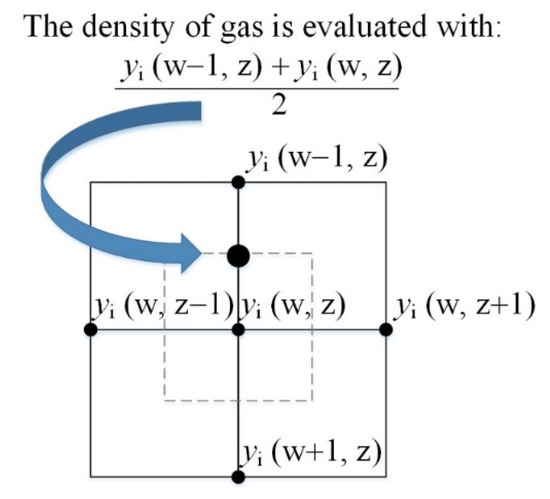
Figure 1.
Illustration of the discretization mesh of species/mass conservation equation.
2.3. Conservation of Charge
The charge transfer through the modeled SOFC is described by different charge exchange mechanisms that are modeled in the following subsections. A schematic diagram is shown in Figure 2 to illustrate these mechanisms. Each number (1–5) in Figure 2 depicts the mechanism that is described in the equally numbered subsection.
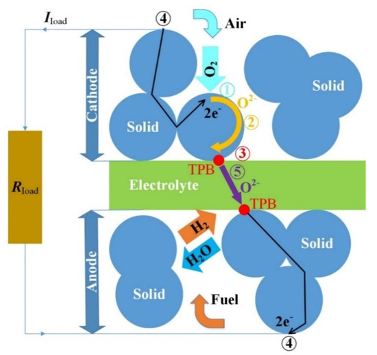
Figure 2.
Illustrated charge transfer within the solid oxide fuel cell (SOFC).
2.3.1. Surface Exchange
It is assumed the oxygen (O2) that fills the pores of solid (i.e., mixed ionic-electronic conductive—MIEC)) material is adsorbed into the cathode surface. Oxygen ions (O2−) are formed with a double negative charge by accepting electrons (e−) from the cathode. The flow of O2− (JO2−) can be modeled as follows [16]:
The surface exchange coefficient is denoted with ksurf. It depends on the temperature and the partial pressure of O2. The equilibrium oxygen ion concentration is denoted with CO2−, eq and depends on the partial pressure of O2 within pores. The concentration of oxygen ions (CO2−) decreases during the increasing electric current load (CO2− < CO2−, eq).
2.3.2. Bulk Diffusion
Since the electronic conductivity of the cathode MIEC material is high and should not limit the electric current, the diffusion of O2− is assumed to limit the current. The diffusion of O2− is modeled by using Fick’s first law:
Dchem is chemical diffusion coefficient that depends on temperature and partial pressure of O2 [17].
2.3.3. Charge Transfer
At the interface between the solid MIEC and electrolyte material the O2− are exchanged. The local charge transfer voltage (overpotential) is the driving force for this process [17]. The current density is modeled by the Butler–Volmer equation:
The anode/cathode exchange current density is denoted with i0,a/c, forward/backward exponential coefficient of anode/cathode with (for simplicity, , , , are used), Vs is solid potential, Vel is electrolyte potential, and V0,a/c is anode/cathode potential that can be obtained from Nernst equation, respectively.
Partial pressures of oxygen, hydrogen and water are denoted with pO2, pH2, and pH2O, respectively, and the ΔGH2 denotes Gibbs free energy for hydrogen. The temperature coefficient kth is calculated from Equation (17), considering open circuit voltage of measured SOFC (OCV = V0,c − V0,a), operating temperature, and partial pressures (or mass fractions) of gas species.
2.3.4. Electronic Current
Electronic current is modeled in solid MIEC material of the cathode by the continuity equation [17]:
The electronic conductivity of cathode MIEC material is denoted with σs,c, δads denotes delta function:
Similarly, the electronic current is modeled in solid MIEC material of anode:
The electronic conductivity of anode MIEC material is denoted with σs,a, δa denotes delta function.
2.3.5. Ionic Current
The ionic current in anode/cathode/electrolyte is modeled with the continuity equation [17]:
The ionic conductivity of anode/cathode/electrolyte is denoted with σion,a/c/el, δa/c denotes delta function.
2.4. Boundary Conditions
Boundary conditions (BCs) have to be specified at different interfaces of the modeled SOFC structure in order to obtain a closed solution of the system of coupled partial differential equations. Figure 3 shows the interfaces A–K within the modeled domain, whereas a description of BCs at these interfaces is given in Table 1.
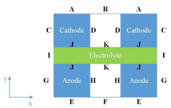
Figure 3.
Schematic of interfaces in the modeled domain.

Table 1.
The boundary conditions.
2.5. Modeled Structure
An image of a SOFC cross-section profile was used to define the geometry of modeled domains (cathode, electrolyte, and anode) within the SOFC. The image had to be processed properly to detect the three different phases (solid, electrolyte, and gas) present within the real SOFC. Different image processing algorithms can be found in the literature [18,19,20]. Many ideas of how to choose a global threshold have been already presented [19]. Most of these methods derive the threshold value using the properties of an image histogram. A similar problem of how to detect different phases from threshold values has been already addressed in Ref. [20]. It is assumed that the grey values of the phases are normally distributed and sufficiently apart from each other. Hence their superposition results in a local minimum between the two phases when inspected in the pixel histogram [20].
A simple algorithm for detecting the three different phases was developed in our case. First, a vector with 256 locations was created. Second, the pixels in the image that have a certain grey scale value (GSV) were counted and the sum was stored at the GSV-th location in the vector. This procedure was repeated for each GSV ∈ [0,1,…,255]. Third, three local maximums of the vector were sought. Each GSV at which a local maximum was found corresponded to one of the three different phases, considering these phases had normal distribution of the pixel number with respect to this GSV. Fourth, two local minimums were sought by considering each one as located between two maximums. Fifth, two threshold values were obtained from indexes of the locations in the vector, at which two local minimums were found. An example of detection of two threshold values that differentiate the three different phases from the grey-scale image is shown in Figure 4.
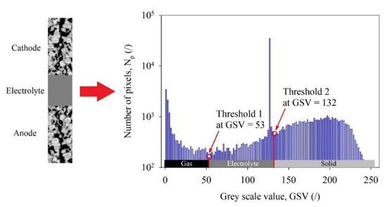
Figure 4.
Detection of two threshold values to differentiate three phases from a grey-scale image [10].
2.6. Solid-Electrolyte-Gas Interfaces
Three different phases (solid, electrolyte, and gas phases) were initially set to zero values at each discretized location (w, z) of the modeled SOFC. These phases had to be unambiguously determined based on two threshold values, which were resolved as described in Section 2.5. The following criteria were considered:
- if (GSV < Threshold 1) then Gas (w, z) = 1;
- else if ((GSV ≥ Threshold 1) and (GSV < Threshold 2)) then Electrolyte (w, z) = 1;
- else Solid (w, z) = 1;
In the next step, only the connected (percolated) solid and electrolyte phases were determined in between the electric contacts, which were denoted as interfaces A and E in Figure 3. The connected gas phases to interface B and F were determined. For example, delta function δa/c (w, z) = 1 since TPB was active within the porous anode or cathode if all three phases ere percolated and met in a single point (w, z). Otherwise, δa/c (w, z) = 0 since TPB was inactive. This situation is shown schematically in Figure 5a. The upper part of Figure 5b shows active TPBs within the modeled SOFC. The lower part of Figure 5b shows the actual 2-D profile of the mass fraction (Y) of O2 and H2 that corresponds to the percolated gas phase within the porous cathode and anode, respectively, as seen in the upper part. Please note that TPB detection actually needs four neighboring pixels (i.e., a small image of 2 × 2 pixels) that represent different phases. It is obvious that TPB detection strongly depends on both threshold levels. Consequently, there is some uncertainty in this kind of detection, as it is impossible to determine whether a TPB at the interface really exists or not. Moreover, the reconstruction of porous material in this paper was based on the 2-D grey-scale image, which may introduce additional uncertainty. Detailed analysis and detection of TPB would require three-dimensional (3-D) tomography techniques, e.g., focused ion beam-scanning electronic microscopy (FIB-SEM) [21] and X-ray computed tomography (CT) [22]. Those provide more accurate SOFC microstructure characterization. These cutting-edge 3-D characterization techniques are very expensive and time-consuming [23]. This is why the detection in our case was restricted to 2-D grey-scale images only.
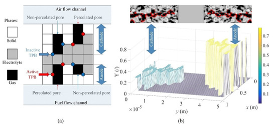
Figure 5.
(a) Schematic explanation of the detection of active triple phase boundary (TPB) and (b) percolated gas phases.
2.7. The Degradation Model
Degradation mechanisms of SOFC have been studied experimentally [24,25] and theoretically [11] to investigate how the microstructure evolves over long-term operation under different conditions, such as temperature, current density [24,25], and initial composition of the porous anode, and the average size of Ni and YSZ grains within the microstructure [11].
Since a real SOFC operates at high temperatures (at T = 800–1000 °C), the microstructure evolution, such as grain growth or particle coarsening, is significant [11]. The microstructure becomes increasingly coarser and denser with increasing testing temperature, current density, and testing time [24]. At 750 °C an increase in grain size occurs mainly in the bulk and interface compared with a non-degraded cell. At 850 °C and above, the grain coarsening in the bulk becomes more pronounced than at 750 °C. The coarsened interface region is about 1–2 μm in width at 850 °C and up to 5 μm at 950 °C. It was also seen that at 850 °C the process of grain coarsening and interface densification continues with increasing testing time up to 17,500 h [24]. From these results one can note that microstructure evolution generally progresses with increasing temperature and testing time. Ostwald-ripening is an important mechanism of Ni coarsening in SOFC anode [26]. It occurs due to the transport of volatile Ni species via the gas phase and diffusion of vacancies, driven by different grain sizes.
Despite the detailed studies, only a few papers [27,28] deal with the problem of how the microstructural degradation actually affects the electric performance of SOFC. In this paper the electric performance of a degraded SOFC was calculated by adjusting fewer parameters compared to the number of parameters that need to be set in the phase field model [11]. Moreover, the validation of such a model would require detailed analysis with three-dimensional (3-D) tomography techniques. These techniques have shown that the Ni (YSZ) grains grow exponentially with time [9]. Therefore, the degradation of SOFC due to grain growth was modeled by considering the power law [9]:
Time-dependent diameter of Ni grains is denoted with d, initial diameter with d0, growth coefficient with k and time with t. The exponential coefficient is denoted with κ. It equals 2 for grain growth and 3 for particle coarsening due to Ostwald-ripening [11].
However, Equation (22) has to be slightly adapted for numerical implementation. It is assumed that d0 is determined by the minimum distance between the two adjacent points where active TPBs are located. This simplification is done due to problems with detecting grain boundaries of the Ni (YSZ) particles and their actual diameter by processing a grey-scale image. Moreover, reconstruction of the porous anode according to the phase field model would be necessary if actual grain growth was considered rigorously [11]. That is beyond the scope of the present paper, so the following algorithm was proposed.
First, the active TPBs are resolved as described in Section 2.6. Second, two vectors are defined for storing two distances (d1,min, d2,min) from one to the closest two TPB points. Third, d1,min and d2,min are found. Fourth, the SOFC model is evaluated at each iteration (q) using a fixed time step (Δt). Fifth, the following condition is checked at each iteration and at each active TPB point:
This algorithm runs iteratively as long as it is defined by a maximum number of iterations q. It should be noted that after a certain number of iterations, the condition in Equation (23) is fulfilled at some active TPB point and this TPB is deactivated (δa (w, z) = 0). In this way, the particle diameter is increased. It is important to note the number of active TPBs is decreased, so this model enables fitting the parameters k and n to achieve good approximation to results of measured or calculated relative TPB density from the literature [10,11].
2.8. Model Parameters
Detailed descriptions of measured SOFC, including the lanthanum strontium cobalt ferrite (LSCF) cathode, Ni-scandia stabilized zirconia (Ni-SSZ) active (or support) anode layer, and electrolyte bilayer, can be found in Ref. [10]. The physical parameters are adopted from the literature, or fitted to match the desired characteristics of measured SOFC. Table 2 shows the list of input parameters.
Table 2.
Input parameters of the SOFC model.
3. Results and Discussion
The SOFC electric performance is simulated by using the model according the parameters in Table 2. We start with AC analysis because it is intended to adjust the anode/cathode exchange current density (i0,a/c) and qualitatively validate the simulation results with measured electro-impedance spectrum (EIS) in Ref. [10]. Note that the adjustment of i0,a/c should be done initially for online application of the model in practice, by fitting the calculated and measured EIS. Exact fitting of the EIS was not of the primary concern in this study case, but rather to achieve similar trends of simulated and measured EIS curves.
3.1. AC Analysis
The modeled cell was perturbed at OCV, according to the measurement results in Ref. [10], with sinusoidal voltage with the amplitude 14 mV. The frequency (f) of voltage signal was set to each of 31 logarithmically equally spaced values of frequency from 0.1 Hz to 100 Hz to simulate the EIS. The temperature was set to 900 °C. Other input parameters of the model can be found in Table 2. Figure 6 shows EIS of (a) non-degraded (i.e., at time t = 0 h) and (b) degraded SOFC (i.e., at time t = 1000 h). The low-range frequency arc was attributed to the anode charge transfer, whereas the mid-range frequency arc was correlated with charge transfer and surface exchange process in the cathode.
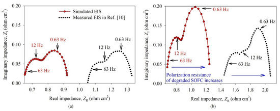
Figure 6.
Electro-impedance spectrum (EIS) of (a) non-degraded SOFC (at time t = 0 h) and (b) degraded SOFC (at time t = 1000 h). Three different frequencies (f = 0.63, 12, and 63 Hz) are labeled for guidance.
The anode and cathode polarization resistances increase over time (i.e., from 0 to 1000 h) due to the reduced density of TPBs within the anode and cathode. The increased polarization resistance of the degraded SOFC indicated a correct trend regarding the time evolution of measured EIS, as can also be seen in Figure 8c in Ref. [10]. The measured series resistances were higher than in this case, which may be attributed to the wiring and contact resistances, which were not considered in the presented model. Moreover, if considering only the series resistances (about 1.05 Ω cm2 at non-degraded and 1.4 Ω cm2 at the degraded cell) that can be deduced from measured EIS, the voltage drop of SOFC would be about 0.47 V and 0.63 V at the current density (J) of 0.45 A cm−2, so the direct current (DC) voltage of the SOFC (Vcell) should be lower than shown in Figure 8a in Ref. [10]. The measured Vcell of non-degraded SOFC was about 0.56 V (at time t = 0 h), whereas Vcell of degraded SOFC was about 0.42 V (at time t = 1000 h).
Since the open circuit voltage (OCV) of SOFC is about 0.97 V, the measured Vcell should have been 0.50 V and 0.34 V when the aforementioned voltage drops were considered, respectively. Due to these discrepancies, the model was fitted only to reproduce the degradation of Vcell, as presented in Section 3.2, since we focus on calculating the electric performance of SOFC over time. However, a profound inspection of the measurement equipment and physical parameters of the real SOFC device would be necessary to obtain a better fitting of EIS, whereas a comparison of impedances could be done only if detailed measurement data were available in Ref. [10].
3.2. DC Analysis
In the second set of experiments, the DC analysis was performed. A comparison between calculated and measured electric performance of SOFC was done to address more realistic degradation due to the coarsening of Ni particles within the anode. A fraction of backscattered electron (BSE) microscope pictures were taken from Figure 3a in Ref. [10] to define an approximation to the real structure of porous anode. The experimental degradation test was performed for 1000 h at the temperature of 900 °C and at current density of 0.45 A cm−2, whereas 3 vol% humidified H2 was supplied to the anode and air was supplied on the cathode side. The flow rates of hydrogen and air were 350 cm3 min−1 and 1500 cm3 min−1, respectively [10]. Due to this, the temperature and current density of the modeled SOFC was set to Tcell = 900 °C and Jcell = 0.45 A cm−2, respectively, during the simulation from 0 to 1000 h. Time increment Δt = 100 h was used since the experimental data was defined at 100 h intervals in Ref. [10]. The anode exponential coefficient (κa = 3) and the anode growth coefficient (ka = 2.1 × 10⁻²¹ m3 h−1) were manually fitted to match the relative TPB density of the measured SOFC in Ref. [10].
Figure 7a shows relative TPB density in the anode (TPBa) and in the cathode (TPBc) as a function of time. The calculated relative TPBa density had a similar profile as that in Figure 8d in Ref. [10]. The initial absolute value of TPBa (t = 0 h) was approximately four times lower (0.7 μm−2 vs. 2.9 μm−2), but another study revealed [30] that the density of active TPBs may be lower (0.74 μm−2). Since the TPBs that lie in the third dimension (i.e., in the plane of 2-D grey-scale image) cannot be resolved with our algorithm, it was obvious why the obtained density of TPBs from 2-D grey-scale image was lower. Although the TPB density was lower in our case than it should have been (or than it was in the real SOFC), it could be compensated for with higher activity of TPBs (i.e., higher exchange current density, i0,a/c) to achieve a similar electric performance of modeled SOFC. It is important to note the presented model approximated the spatial distribution of TPBs in real SOFC. Due to this, it could be expected that the simulation results may be more reliable compared to those obtained with 0-D or 1-D models.
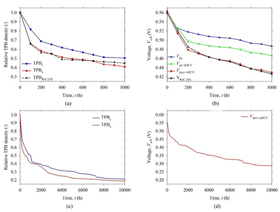
Figure 7.
(a) Relative TPB density and (b) output voltage (Vcell) of the SOFC as a function of time from 0 to 1000 h. (c) Relative TPB density and (d) output voltage (Vcell) of the SOFC as a function of time from 0 to 10,000 h. The anode and cathode exponential coefficients, κa = 3 and κc = 3, and the anode and cathode growth coefficients, ka = 2.1 × 10⁻²¹ m3 h−1 and kc = 1.4 × 10⁻²¹ m3 h−1, are considered.
Figure 7b shows the calculated voltage (Vda) of SOFC, with degraded anode, which is almost the same as the reference voltage (VRef.[10] in Figure 8a in Ref. [10]) from 0 to 100 h, whereas a higher voltage difference (0.03–0.06 V) were noticed from 200 h to 1000 h. This difference may be partly attributed to a noticeable drop of open circuit voltage (ΔOCV = 0.02 V) that occurs in real SOFC at t = 200 h, as seen in Figure 8a in Ref. [10], and partly to some other degradation processes that possibly were going on concurrently. The ΔOCV was attributed to different agents. Since OCV = V0,c − V0,a depends on mass fraction of hydrogen (y0, H2), referring to Equation (17), it can be speculated that y0, H2 was slightly decreased due to increased humidity in the fuel or hydrogen gas leak. To achieve this, the input molar fraction of hydrogen (x0, H2) was adjusted to 0.955 in order to simulate ΔOCV at t = 200 h.
The voltage (Vda+ΔOCV) of SOFC, with degraded anode and ΔOCV, followed the reference voltage (VRef. [10]) from 0 to 200 h, but the difference between Vda+ΔOCV and VRef. [10] that remained was probably attributed to some other degradation processes. The grain coarsening possibly occurred in the SOFC cathode due to high temperature (900 °C) [24], although there was no data about it in Ref. [10]. In order to reproduce the higher degradation rate of VRef. [10] the grain coarsening was also modeled in the SOFC cathode (growth coefficient kc = 1.4 × 10⁻²¹ m3 h−1 and cathode exponential coefficient κc = 3) The values were manually fitted to achieve a minimum standard deviation between the voltage (Vda/c+ΔOCV) of SOFC, with degraded anode/cathode and ΔOCV, and VRef. [10]. It should be noted that using the model for online estimation of SOFC degradation would require similar fitting procedure. The parameters ka/c and κa/c should be fitted automatically on the measured voltage profile within the first few 100 h intervals.
In Figure 7b, Vda/c+ΔOCV closely followed VRef. [10] if the degradation due to the grain coarsening was modeled in both electrodes. The maximum absolute difference between the Vda/c+ΔOCV and VRef. [10] was about 7 mV, whereas standard deviation was about 3 mV. Both values were negligibly small. The absolute degradation rate of VRef. [10] from 0 to 1000 h was estimated to be 0.14 V kh−1, whereas the relative degradation rate was about 25% kh−1. The Vda/c+ΔOCV had similar degradation rates. These rates were very high, most probably due to high operating temperature 900 °C, which was close to the melting point of the materials, so the agglomeration of grains progressed very quickly, as already argued in Ref. [10].
After the fitting procedure, the model was used to calculate the degradation of SOFC electric performance in the range of 10,000 h, which was a common operating period [24]. Two additional plots, as seen in Figure 7c,d, were added to show the calculated degradation of the modeled SOFC. It can be noticed that the relative TPB density of anode (cathode) dropped to about 0.18 (0.21), whereas the Vda/c+ΔOCV dropped to about 0.28 V at 10,000 h. In other words, in this period of time, the Vda/c+ΔOCV decreased by approximately 50% if considering the initial Vda/c+ΔOCV value of 0.56 V. To show how the degradation affects the electric conversion efficiency (η) of the SOFC, the η was evaluated at every Δt = 100 h from 0 to 1000 h, according to the following equation:
The Pel is electric power density, Pin is input power density, Φin,H2 is input molar flux of hydrogen. It can be noticed that η depends on the output voltage of SOFC (Vcell), Faraday constant (F), and standard enthalpy of formation for hydrogen (ΔHH2) only if it is assumed that each oxidized H2 contributes two electrons, Equation (2). Figure 8a shows the η of the SOFC as a function of time. The reference conversion efficiency (ηRef. [10]) dropped rapidly from 0 to 200 h and moderately from 200 h to 1000 h (by approximately 0.07 and 0.04, respectively). A similar trend of the conversion efficiency (ηda/c+ΔOCV) of SOFC, with degraded anode/cathode and ΔOCV, was observed. The absolute degradation rate of ηRef. [10] from 0 to 1000 h was estimated to be 0.11 kh−1, whereas the relative degradation rate was about 25% kh−1. Similar degradation rates of ηda/c+ΔOCV were noticed. These values were high, but it should be noted that the real SOFC degradation test was performed at high temperature (900 °C). The details about the experimental test can be found in Ref. [10].
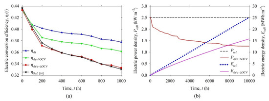
Figure 8.
(a) Electric conversion efficiency (η) of the SOFC as a function of time from 0 to 1000 h. Degradation is considered in the anode (ηda) layer alone, with drop of open circuit voltage (ηda+ΔOCV) and in both, anode and cathode layers, with drop of OCV (ηda/c+ΔOCV). (b) Electric power density (Pcell) and energy yield (Ecell) of non-degraded (Pref, Eref) and degraded SOFC (Pda/c+ΔOCV, Eda/c+ΔOCV) as a function of time from 0 to 10,000 h.
It is important to note that the proposed model reproduces reliable results which are closely related to the measured ones. Figure 8b shows the electric power density (Pcell) and energy density (Ecell) of SOFC that can be calculated by Equations (25) and (26).
The energy yield of non-degraded cell (Eref) equals 25.1 MWh m−2, whereas the energy yield of degraded cell (Eda/c+ΔOCV) equals 15.8 MWh m−2 at t = 10,000 h. The yield of electrical energy, generated by the real SOFC over a long time, would be much lower (by approximately 37%) than calculated by considering the initial electric performance (i.e., the non-degraded SOFC).
As a result, the overall cost per generated MWh of electric energy could be estimated when a high power SOFC generator was considered. This estimation is beyond the scope of the present study since the input data of the model is based on laboratory scale SOFC.
The model is very useful tool to predict the degradation rate and is suitable for online monitoring of the SOFC. However, the proposed Ni coarsening model should be improved in the future in order to consider the temperature, current density, and gas composition dependent growth of particles.
4. Conclusions
In this paper, the reduced-complexity, two-dimensional, microstructural model of solid oxide fuel cells (SOFC) was proposed since a numerically tractable model is sought for online evaluation of SOFC electric performance degradation. The SOFC degradation that occurs at high temperature due to the nickel agglomeration in the anode was modeled by using power law coarsening theory. The model was validated by comparing the electro-impedance spectra (EIS) of the modeled SOFC and measured EIS characteristics. The anode and cathode polarization resistances increased over the simulated time, which indicated the trends which are also observed in the real SOFC device.
The model was also validated based on the measurement data. The modeled structure was based on the backscattered electron (BSE) microscope cross-section picture of the measured SOFC. The input parameters were adjusted according to the known material parameters or fitted to match the relative density of TPBs profile and initial performances of the measured SOFC. The output voltage of the modeled SOFC closely follows the measured voltage from 0 to 1000 h when considering the degradation due to the grain growth in both electrodes. The absolute and relative degradation rate of electric conversion efficiency (η) equals 0.11 kh−1 and 25% kh−1, respectively. The electric energy yield (Ecell) of the degraded SOFC over the simulated time of 10,000 h was about 37% lower than it would be in the Ecell of non-degraded SOFC. Moreover, the overall cost per generated MWh of electric energy could be estimated when considering a commercial SOFC stack for high electric power.
Regarding the presented results, the model was found suitable for online estimation of the degraded SOFC electric performances. Future work is going to improve the proposed degradation model by adding the temperature, current density, and gas composition dependent growth of particles.
Author Contributions
The Author reviewed available literature about modeling and characterization of solid oxide fuel cells, implemented the presented two-dimensional, microstructural model of solid oxide fuel cell in Matlab R2016b, performed extensive searching of input parameters of the model, fitted the model to match calculated and measured characteristics, made all graphic processing of the results, and wrote the entire manuscript. The author have read and agreed to the published version of the manuscript.
Funding
This research received no external funding.
Acknowledgments
The Slovenian Research Agency (ARRS) through Research Program P2-0001 and the project PR-07383 is gratefully acknowledged. The Author would also like to kindly thank Đani Juričić, for fruitful discussions and suggestions that improved the content of this paper.
Conflicts of Interest
The Author declare that there is no conflict of interest regarding the content of this article.
Abbreviation
| 1-,2-,3-D | One-,two-,three-dimensional |
| AC | Alternate current |
| BC | Boundary condition |
| BSE | Backscattered electron |
| CT | Computed tomography |
| DC | Direct current |
| e | Electron |
| FDM | Finite difference method |
| FIB | Focused ion beam |
| GSV | Grey scale value |
| LSCFLSM | Lanthanum Strontium Cobalt FerriteLanthanum Strontium Manganite |
| MIEC | Mixed ionic-electronic conductor |
| NiNi-SSZ | NickelNickel-scandia stabilized zirconia |
| O2− | Oxygen ion |
| OCV | Open circuit voltage |
| S | Sulfur |
| SEM | Scanning electronic microscopy |
| SOFC | Solid oxide fuel cell |
| TPB | Triple-phase boundary |
| X-ray | High-energy electromagnetic radiation |
| YSZ | Yttria-stabilized zirconia |
Appendix A
| Gas Species | |
| CH4 | Methane |
| CO2 | Carbon dioxide |
| CO | Carbon monoxide |
| H2 | Hydrogen |
| H2O | Water |
| N2 | Nitrogen |
| O2 | Oxygen |
| Symbols | |
| Forward anode exponential coefficient | |
| Backward anode exponential coefficient | |
| Forward cathode exponential coefficient | |
| Backward cathode exponential coefficient | |
| δ | Delta function |
| i, j | Indexes of gas species |
| κ | Exponential coefficient |
| κa | Anode exponential coefficient |
| κc | Cathode exponential coefficient |
| Normal unit vector | |
| Quantity | |
| Cdl,a | Double layer capacitance of anode |
| CO2− [mol m−3] | Concentration of oxygen ions |
| d [m] | Diameter of nickel grains |
| Dchem [m2 s−1] | Chemical diffusion coefficient |
| Di,j [m2 s−1] | Diffusion coefficient of gas species |
| E [J m−2] | Energy density |
| ΔGH2 [J mol−1] | Gibbs free energy for hydrogen |
| f [Hz] | Frequency |
| F [A s mol−1] | Faraday constant |
| Φ [mol m−2 s−1] | Molar flux density |
| η [/] | Conversion efficiency |
| ΔH [J mol−1] | Standard enthalpy of formation |
| ia/c [A m−2] | Anode/cathode current density |
| i0,a/c [A m−2] | Anode/cathode exchange current density |
| j [kg m−2] | Diffusive mass flux |
| J [A m−2] | Current density |
| Jcell [A m−2] | Output current density of SOFC |
| ka/c [m3 s−1] | Anode/cathode growth coefficient |
| ksurf [m s−1] | Surface exchange coefficient |
| kth [V K−1] | Temperature coefficient |
| μ [/] | Porosity |
| M [kg mol−1] | Molar mass |
| p [kg m−1 s−1] | Pressure |
| P [W m−2] | Power density |
| ρ [kg m−3] | Density of gas |
| R [J mol−1 K−1] | Ideal gas constant |
| Rs [Ω cm2] | Series resistance |
| δ [S m−1] | Electronic or ionic conductivity |
| S [kg s−1] | Source or sink term |
| t [s] | Time |
| T [K] | Temperature |
| v [m s−1] | Velocity |
| Vcell [V] | Output voltage of SOFC |
| Vel [V] | Electrolyte phase potential |
| Vs [V] | Solid phase potential |
| Vi [m3] | Diffusion volume of i-th gas specie |
| xi [/] | Molar fraction of the i-th gas specie |
| yi [/] | Mass fraction of the i-th gas specie |
| η [/] | Conversion efficiency |
References
- Ali Saadabadi, S.; Thallam Thattai, A.; Fan, L.; Lindeboom, R.E.F.; Spanjers, H.; Aravind, P.V. Solid Oxide Fuel Cells fuelled with biogas: Potential and constraints. Renew. Energy 2019, 134, 194–214. [Google Scholar] [CrossRef]
- Huang, K.; Goodenough, J.B. Direct current (DC) electrical efficiency and power of a solid oxide fuel cell (SOFC). In Solid Oxide Fuel Cell Technology: Principles, Performance and Operations; Woodhead Publishing Limited, Abington Hall, Granta Park, Great Abington: Cambridge, UK, 2009; pp. 141–148. [Google Scholar]
- Chatrattanawet, N.; Saebea, D.; Authayanun, S.; Arpornwichanop, A.; Patcharavorachot, Y. Performance and environmental study of a biogas-fuelled solid oxide fuel cell with different reforming approaches. Energy 2018, 146, 131–140. [Google Scholar] [CrossRef]
- Kupecki, J.; Papurello, D.; Lanzini, A.; Naumovich, Y.; Motylinski, K.; Blesznowski, M.; Santarelli, M. Numerical model of planar anode supported solid oxide fuel cell fed with fuel containing H2S operated in direct internal reforming mode (DIR-SOFC). Appl. Energy 2018, 230, 1573–1584. [Google Scholar] [CrossRef]
- Moçoteguy, P.; Brisse, A. A review and comprehensive analysis of degradation mechanisms of solid oxide electrolysis cells. Int. J. Hydrog. Energy 2013, 38, 15887–15902. [Google Scholar] [CrossRef]
- Papurello, D.; Lanzini, A.; Fiorilli, S.; Smeacetto, F.; Singh, R.; Santarelli, M. Sulfur poisoning in Ni-anode solid oxide fuel cells (SOFCs): Deactivation in single cells and a stack. Chem. Eng. J. 2016, 283, 1224–1233. [Google Scholar] [CrossRef]
- Lanzini, A.; Leone, P.; Guerra, C.; Smeacetto, F.; Brandon, N.P.; Santarelli, M. Durability of anode supported Solid Oxides Fuel Cells (SOFC) under direct dry-reforming of methane. Chem. Eng. J. 2013, 220, 254–263. [Google Scholar] [CrossRef]
- Yu, R.; Guan, W.; Wang, F.; Han, F. Quantitative assessment of anode contribution to cell degradation under various polarization conditions using industrial size planar solid oxide fuel cells. Int. J. Hydrog. Energy 2018, 43, 2429–2435. [Google Scholar] [CrossRef]
- Hubert, M.; Laurencin, J.; Cloetens, P.; Morel, B.; Montinaro, D.; Lefebvre-Joud, F. Impact of Nickel agglomeration on Solid Oxide Cell operated in fuel cell and electrolysis modes. J. Power Sources 2018, 397, 240–251. [Google Scholar] [CrossRef]
- Khan, M.Z.; Mehran, M.T.; Song, R.H.; Lee, J.W.; Lee, S.B.; Lim, T.H. A simplified approach to predict performance degradation of a solid oxide fuel cell anode. J. Power Sources 2018, 391, 94–105. [Google Scholar] [CrossRef]
- Lei, Y.; Cheng, T.L.; Wen, Y.H. Phase field modeling of microstructure evolution and concomitant effective conductivity change in solid oxide fuel cell electrodes. J. Power Sources 2017, 345, 275–289. [Google Scholar] [CrossRef]
- Cuneo, A.; Zaccaria, V.; Tucker, D.; Traverso, A. Probabilistic analysis of a fuel cell degradation model for solid oxide fuel cell and gas turbine hybrid systems. Energy 2017, 141, 2277–2287. [Google Scholar] [CrossRef]
- Zhu, J.; Lin, Z. Degradations of the electrochemical performance of solid oxide fuel cell induced by material microstructure evolutions. Appl. Energy 2018, 231, 22–28. [Google Scholar] [CrossRef]
- Fuller, E.N.; Schettler, P.D.; Giddings, J.C. A new method for prediction of binary gas-phase diffusion coefficients. Ind. Eng. Chem. 1966, 58, 19–27. [Google Scholar] [CrossRef]
- Nerat, M.; Juričić, Ð. A comprehensive 3-D modeling of a single planar solid oxide fuel cell. Int. J. Hydrog. Energy 2016, 41, 3613–3627. [Google Scholar] [CrossRef]
- Søgaard, M.; Vang Hendriksen, P.; Jacobsen, T.; Mogensen, M. Modelling of the Polarization Resistance from Surface Exchange and Diffusion Coefficient Data. In Proceedings of the 7th European SOFC Forum, Lucerne, Switzerland, 3–7 July 2006. [Google Scholar]
- Joos, J. Microstructural Characterisation, Modelling and Simulation of Solid Oxide Fuel Cell Cathodes. In Dissertation, Karlsruher Institut für Technologie, KIT-Fakultät für Elektrotechnik und Informationstechnik; D-KIT Scientific Publishing: Karlsruhe, Germany, 2017. [Google Scholar]
- Otsu, N. A threshold selection method from gray-level histogram. IEEE Trans. Syst. Man Cybern. 1979, 9, 62–66. [Google Scholar] [CrossRef]
- Sahoo, P.K.; Saltani, S.; Wong, A.K.C. A survey of thresholding techniques. Comp. Vis. Graph. Image Process. 1988, 41, 233–260. [Google Scholar] [CrossRef]
- Münch, B.; Holzer, L. Contradicting Geometrical Concepts in Pore Size Analysis Attained with Electron Microscopy and Mercury Intrusion. J. Am. Ceram. Soc. 2008, 91, 4059–4067. [Google Scholar] [CrossRef]
- Wilson, J.R.; Kobsiriphat, W.; Mendoza, R.; Chen, H.Y.; Hiller, J.M.; Miller, D.J.; Thornton, K.; Voorhees, P.W.; Adler, S.B.; Barnett, S.A. Three-dimensional reconstruction of a solid-oxide fuel-cell anode. Nat. Mater. 2006, 5, 541–544. [Google Scholar] [CrossRef]
- Izzo, J.R.; Joshi, A.S.; Grew, K.N.; Chiu, W.K.S.; Tkachuk, A.; Wang, S.H.; Yun, W. Nondestructive Reconstruction and Analysis of SOFC Anodes Using X-ray Computed Tomography at Sub-50 nm Resolution. J. Electrochem. Soc. 2008, 155, B504–B508. [Google Scholar] [CrossRef]
- Yan, Z.; He, A.; Hara, S.; Shikazono, N. Modeling of solid oxide fuel cell (SOFC) electrodes from fabrication to operation: Correlations between microstructures and electrochemical performances. Energy Convers. Manag. 2019, 190, 1–13. [Google Scholar] [CrossRef]
- Liu, Y.L.; Thydén, K.; Chen, M.; Hagen, A. Microstructure degradation of LSM-YSZ cathode in SOFCs operated at various conditions. Solid State Ion. 2012, 206, 97–103. [Google Scholar] [CrossRef]
- Zekri, A.; Knipper, M.; Parisi, J.; Plaggenborg, T. Microstructure degradation of Ni/CGO anodes for solid oxide fuel cells after long operation time using 3D reconstructions by FIB tomography. Phys. Chem. Chem. Phys. 2017, 19, 13767–13777. [Google Scholar] [CrossRef] [PubMed]
- Holzer, L.; Iwanschitz, B.; Hocker, T.; Münch, B.; Prestat, M.; Wiedenmann, D.; Vogt, U.; Holtappels, P.; Sfeir, J.; Mai, A.; et al. Microstructure degradation of cermet anodes for solid oxide fuel cells: Quantification of nickel grain growth in dry and in humid atmospheres. J. Power Sources 2011, 196, 1279–1294. [Google Scholar] [CrossRef]
- Bertei, A.; Nucci, B.; Nicolella, C. Microstructural modeling for prediction of transport properties and electrochemical performance in SOFC composite electrodes. Chem. Eng. Sci. 2013, 101, 175–190. [Google Scholar] [CrossRef]
- Lay-Grindler, E.; Laurencin, J.; Villanova, J.; Cloetens, P.; Bleuet, P.; Mansuy, A.; Mougin, J.; Delette, G. Degradation study by 3D reconstruction of a nickel-yttria stabilized zirconia cathode after high temperature steam electrolysis operation. J. Power Sources 2014, 269, 927–936. [Google Scholar] [CrossRef]
- Brune, A.; Lajavardi, M.; Fisler, D.; Wagner, J.B. The electrical conductivity of yttria-stabilized zirconia prepared by precipitation from inorganic aqueous solutions. Solid State Ion. 1998, 106, 89–101. [Google Scholar] [CrossRef]
- Cronin, J.S.; Wilson, J.R.; Barnett, S.A. Impact of pore microstructure evolution on polarization resistance of Ni-Yttria-stabilized zirconia fuel cell anodes. J. Power Sources 2011, 196, 2640–2643. [Google Scholar] [CrossRef]
© 2020 by the author. Licensee MDPI, Basel, Switzerland. This article is an open access article distributed under the terms and conditions of the Creative Commons Attribution (CC BY) license (http://creativecommons.org/licenses/by/4.0/).