Soc Estimation of the Lithium-Ion Battery Pack using a Sigma Point Kalman Filter Based on a Cell’s Second Order Dynamic Model


Abstract
1. Introduction
2. The Second Order Dynamic Model of the Cell and the Model of the LiBP
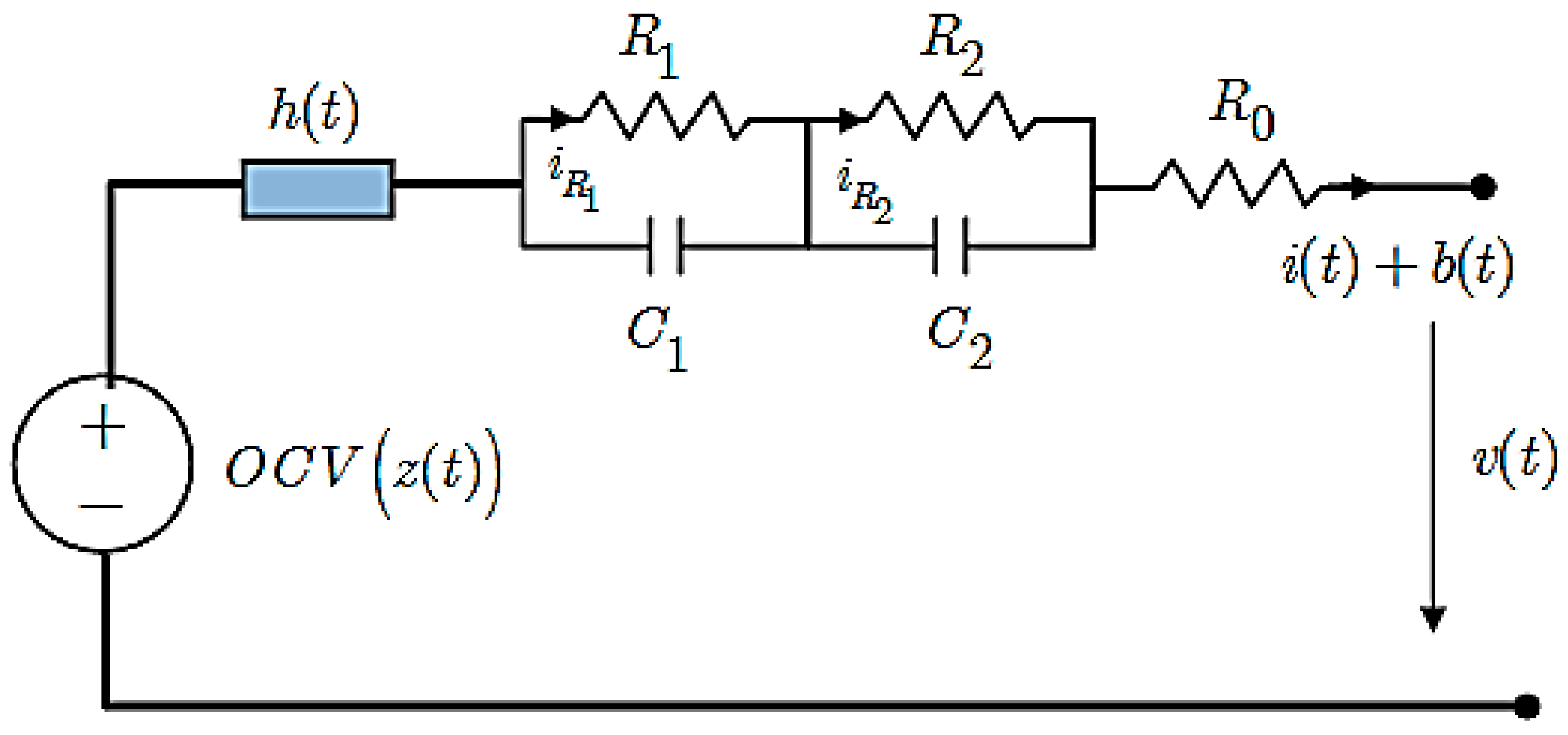
2.1. The Second Order Dynamic Model of the Cell Influenced by Voltage Noise, Noise and Current Bias
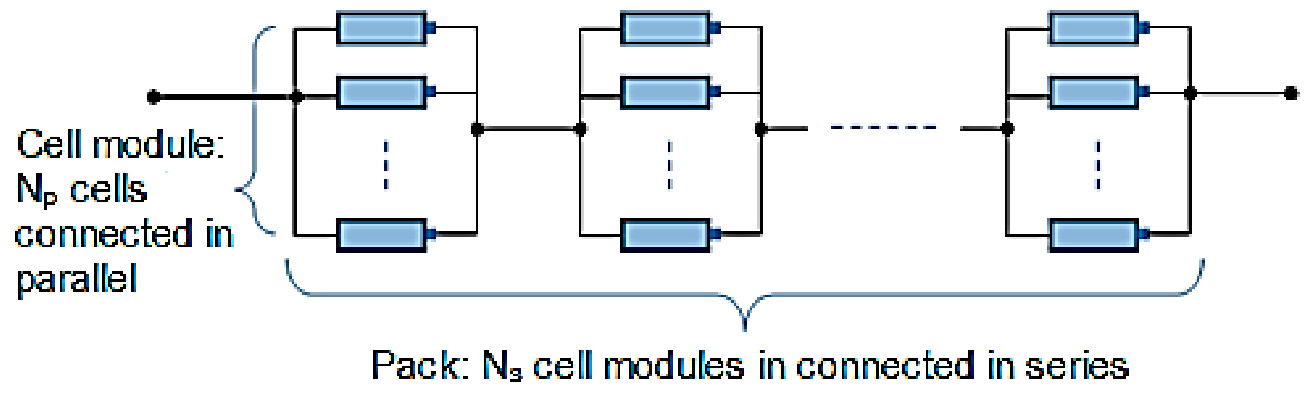
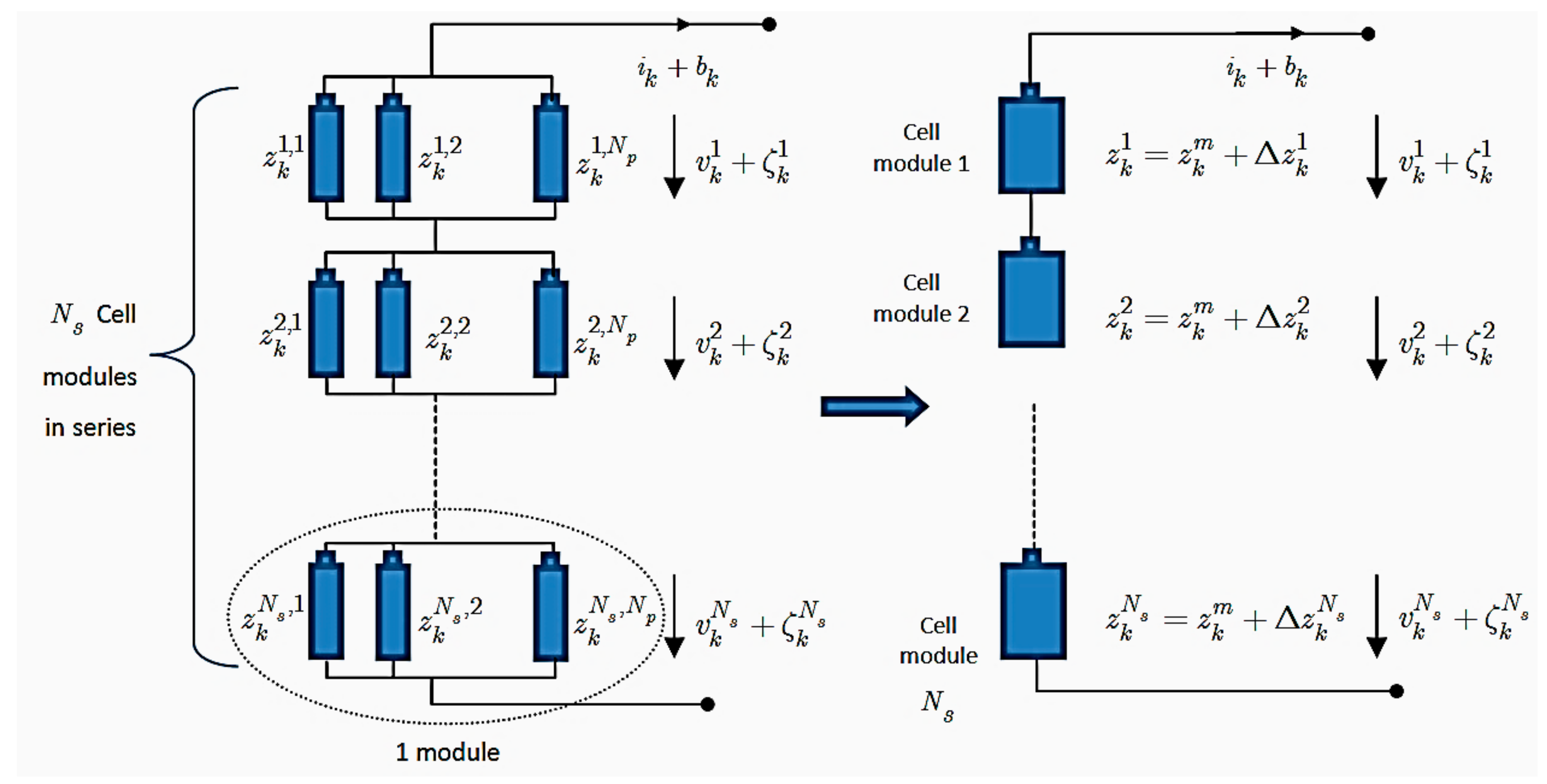
2.2. The Model of LiBP
3. Soc Estimation for the LiBP Using the SPKF
The General Algorithms
| SoC Estimation Algorithm for LiBP. |
| Initialize the parameters of cell Initialize the parameters of LiBP including: , Initialize the covariance matrices Calculate the initial SoC of the cell modules in the LiBP Calculate the internal resistance of the cell modules Calculate the capacity of the cell module |
| For sample time k = 1 to ∞ do |
| Measure the current through the LiBP Measure the voltages on the cell modules Measure the temperature Estimate the state for equivalent cell and estimate the bias current by using the algorithm SPKF 1 |
| For cell module i = 1 to do |
| Estimate the SoC difference of cell module by using the algorithm SPKF 2 |
| End |
| Calculate the SoC for all cell modules |
| End |
| The algorithm SPKF 1 and SPKF 2 are presented in the Appendix A. |
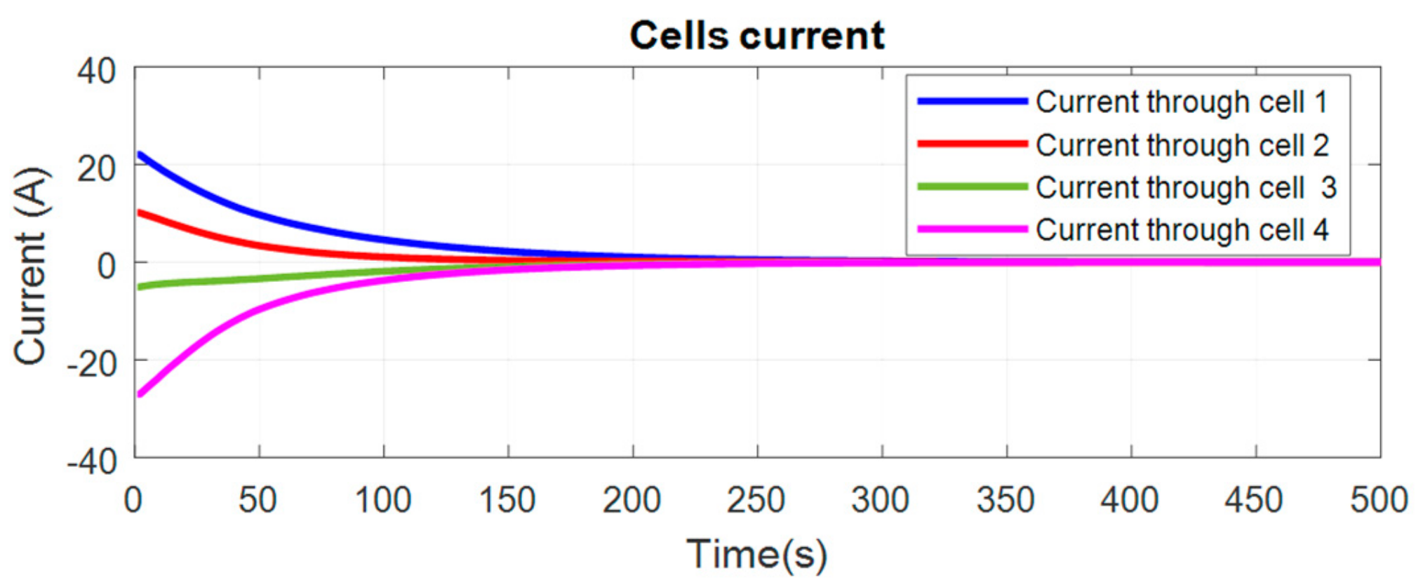
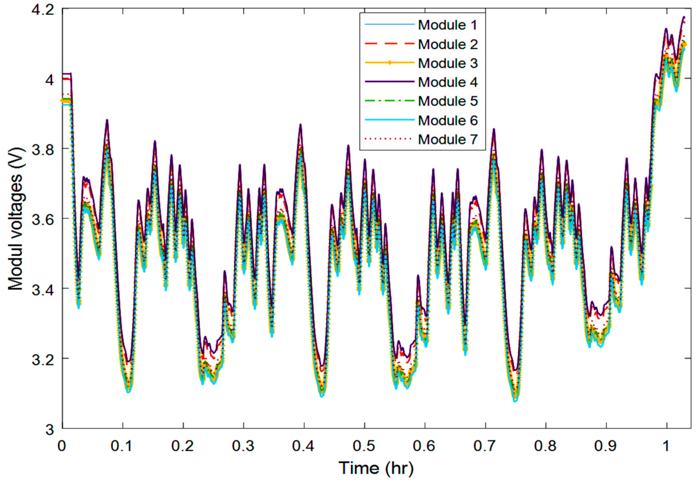
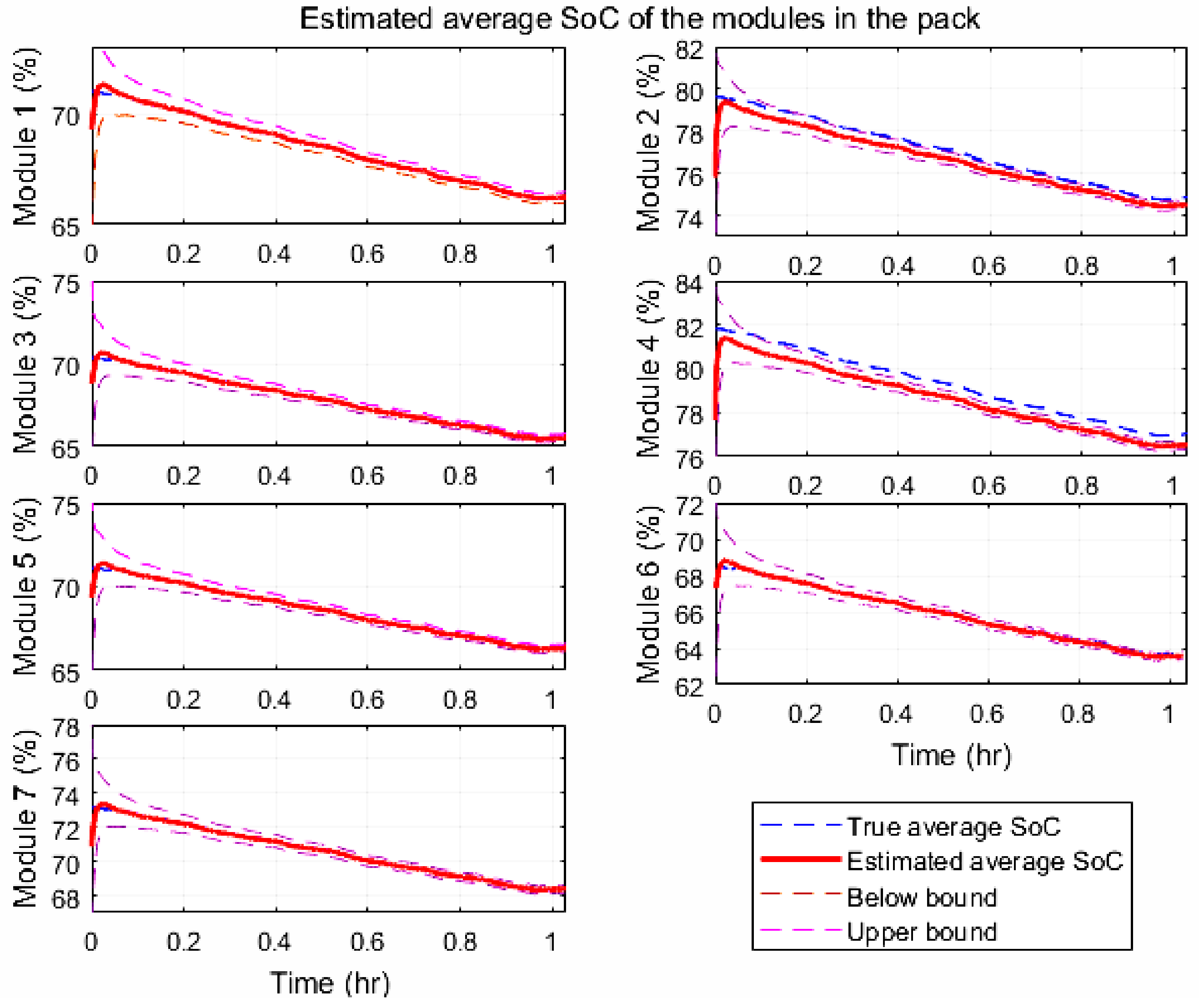
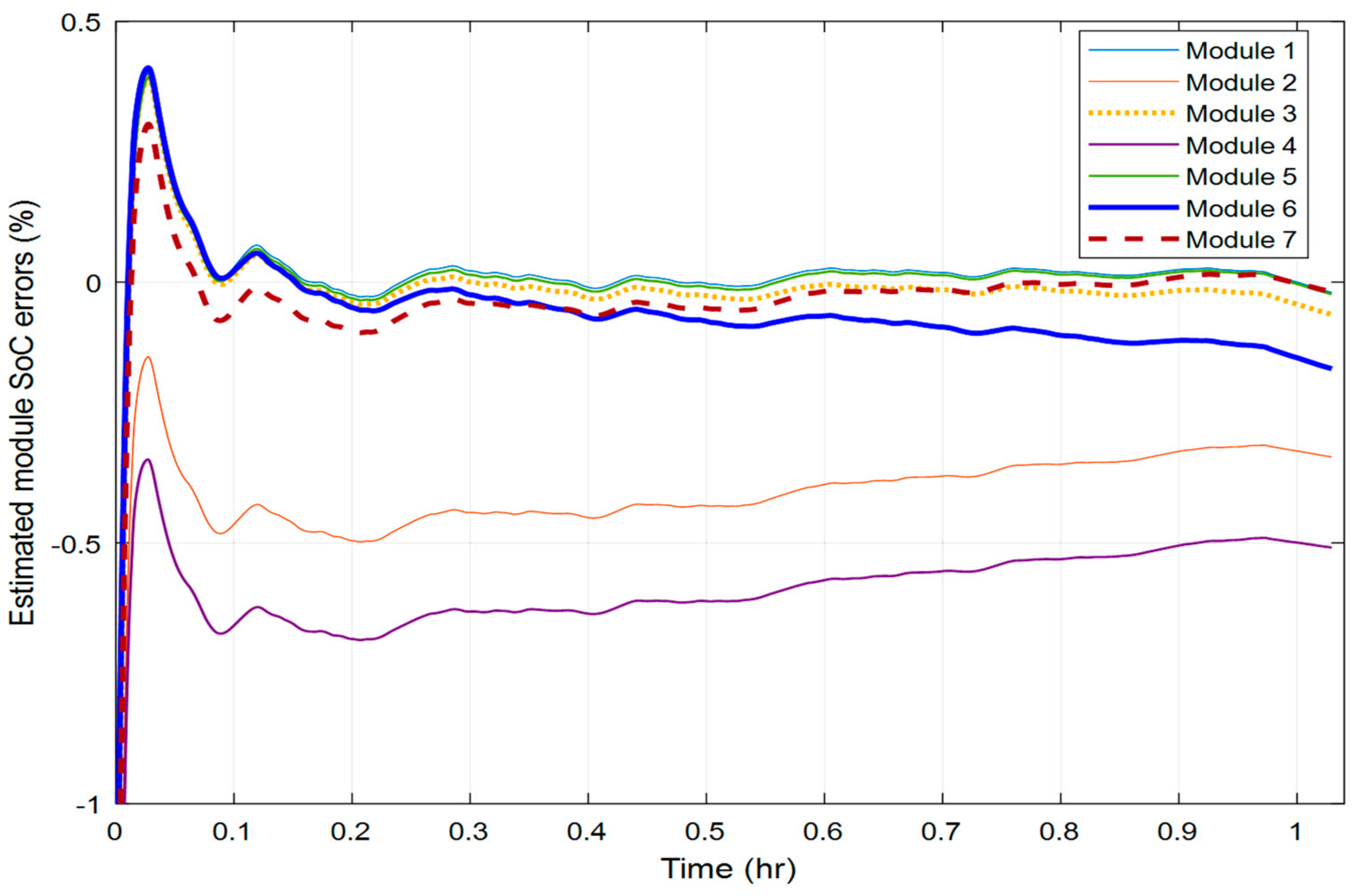
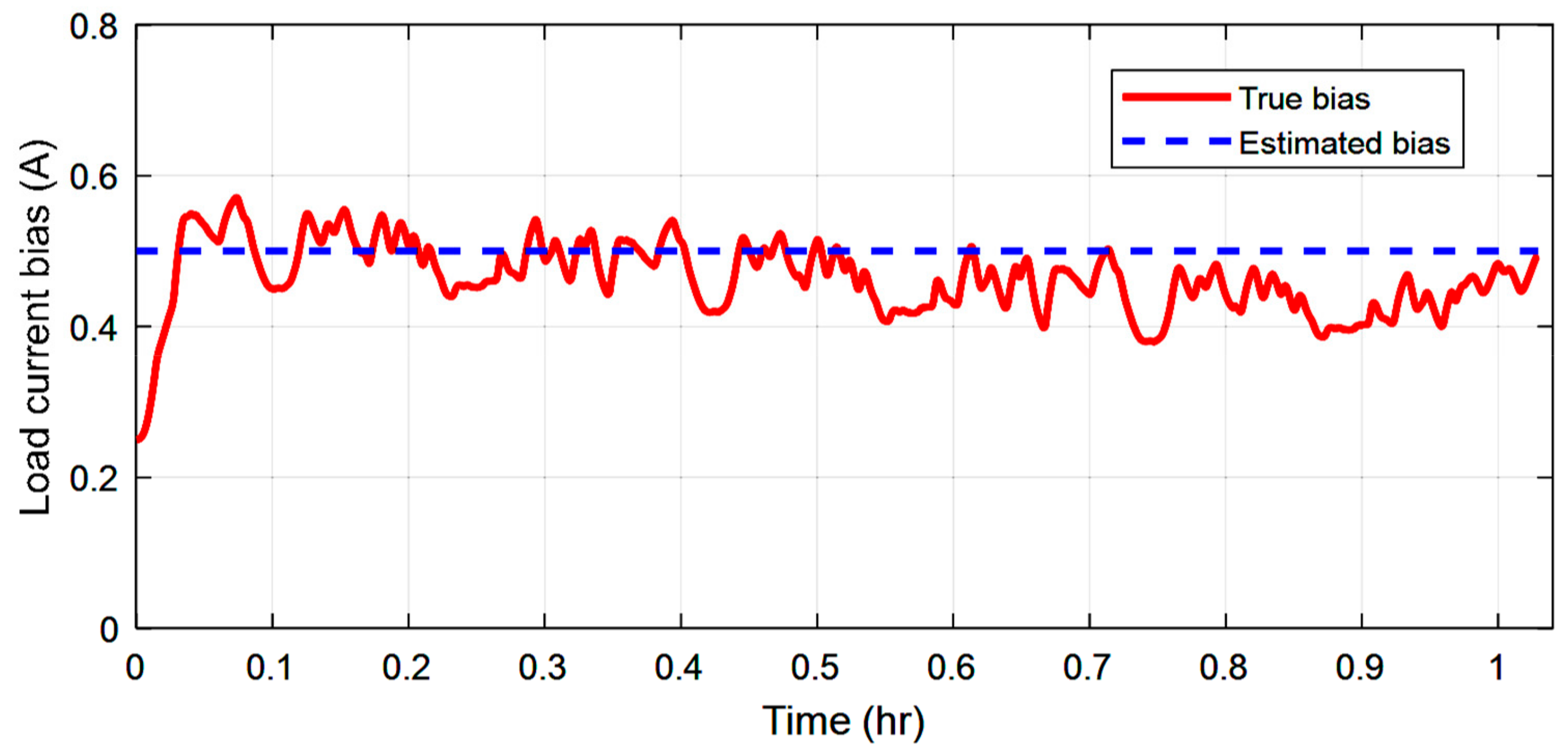
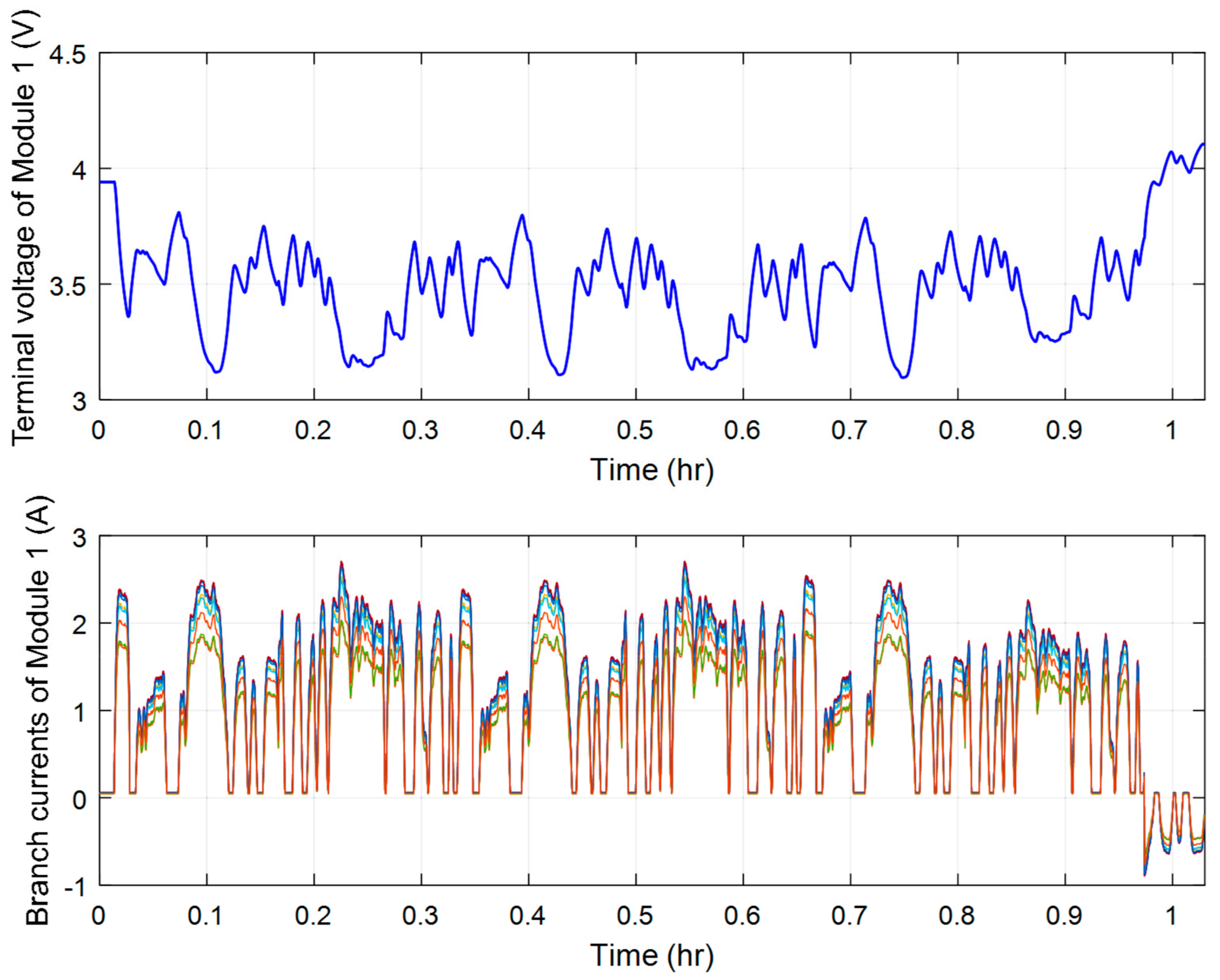
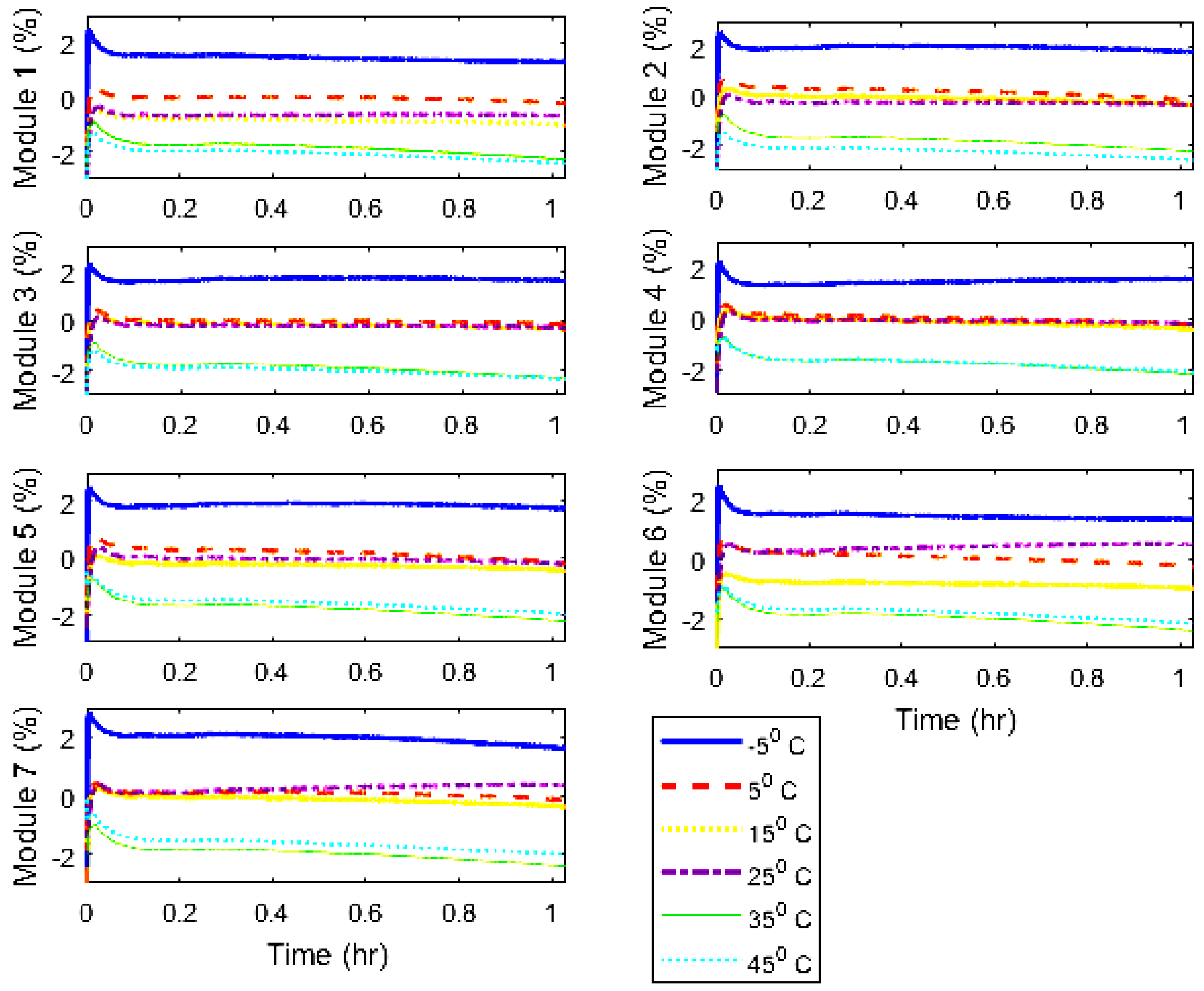
4. The Experimental Results
5. Conclusions
Author Contributions
Funding
Acknowledgments
Conflicts of Interest
Appendix A
Appendix A.1. The Algorithm SPKF 1
- This forms the augmented state vector at the sampling time, including the estimated states at the sample time , the vector of mean values of the system noise and measurement noise :
- This forms the estimated covariance matrix of the state vector estimation error, including the covariance matrices of the state estimation error at time , the noise error and the measured error, respectively.
- The input sigma point matrix containing sigma points is established as
- Calculates state sigma point matrix by using the dynamic state Equation (5):
- The priori state vector estimation is calculated as:
- Update the covariance matrices of the state vector estimation error:
- Calculate the output sigma point matrix using the output equation of Equation (5):
- Estimate the voltage of the equivalent cell.
- Update the covariance matrices of estimated output voltage.
- Update the covariance matrices of the state vector estimation error and output voltage estimation error:
- Calculate the estimation gain matrix as
- Update the priori estimation states by taking into account the output errors, the estimation of state vector as
- Update the covariance matrix of the state vector estimation errors:
Appendix A.2. The Algorithm SPKF 2
- Form the augmented state vector of cell module , including the SoC difference and mean of the SoC difference noise :
- Form the covariance matrix of the SoC difference estimation error:
- The input sigma point matrix containing sigma points is established as
- Calculate the state sigma point matrix.with .
- Calculate the priori SoC difference estimation.
- Update the covariance matrix of SoC difference estimation error.
- Calculate the output sigma point matrix.
- Estimate the output voltage.
- Update the covariance matrix of the output voltage estimation error.
- Update the covariance matrix of SoC difference estimation error and output voltage estimation error.
- Calculate the estimation gain matrix as
- SoC difference estimation is calculated as
- Update the covariance matrix of SoC difference estimation error.
Appendix A.3. Tables A1–A3

| Cell1 | Cell2 | Cell3 | Cell4 | Cell5 | Cell6 | Cell7 | Cell8 | Cell9 | |
|---|---|---|---|---|---|---|---|---|---|
| Module 1 | 0.49 | 0.69 | 0.63 | 0.99 | 0.52 | 0.80 | 0.80 | 0.71 | 0.54 |
| Module 2 | 0.78 | 0.6 | 0.98 | 0.74 | 0.64 | 0.47 | 0.71 | 0.44 | 0.80 |
| Module 3 | 0.56 | 0.88 | 0.99 | 0.96 | 0.99 | 0.42 | 0.56 | 0.93 | 0.44 |
| Module 4 | 0.67 | 0.99 | 0.79 | 0.83 | 0.64 | 0.77 | 0.98 | 0.60 | 0.57 |
| Module 5 | 0.90 | 0.50 | 0.92 | 0.70 | 0.80 | 0.74 | 0.72 | 0.54 | 0.57 |
| Module 6 | 0.52 | 0.54 | 0.64 | 0.78 | 0.94 | 0.98 | 0.42 | 0.47 | 0.90 |
| Module 7 | 0.59 | 0.82 | 0.78 | 0.93 | 0.99 | 0.85 | 0.82 | 0.59 | 0.67 |
| Cell1 | Cell2 | Cell3 | Cell4 | Cell5 | Cell6 | Cell7 | Cell8 | Cell9 | |
|---|---|---|---|---|---|---|---|---|---|
| Module 1 | 0.0013 | 0.0014 | 0.0011 | 0.0015 | 0.0010 | 0.0010 | 0.0013 | 0.0011 | 0.0012 |
| Module 2 | 0.0014 | 0.0011 | 0.0013 | 0.0011 | 0.0013 | 0.0012 | 0.0011 | 0.0014 | 0.0011 |
| Module 3 | 0.0014 | 0.0014 | 0.0012 | 0.0014 | 0.0014 | 0.0011 | 0.0013 | 0.0011 | 0.0015 |
| Module 4 | 0.0013 | 0.0012 | 0.0012 | 0.0014 | 0.0015 | 0.0014 | 0.0013 | 0.0014 | 0.0010 |
| Module 5 | 0.0011 | 0.0014 | 0.0014 | 0.0012 | 0.0010 | 0.0012 | 0.0014 | 0.0013 | 0.0014 |
| Module 6 | 0.0011 | 0.0012 | 0.0013 | 0.0013 | 0.0013 | 0.0013 | 0.0012 | 0.0015 | 0.0014 |
| Module 7 | 0.0011 | 0.0011 | 0.0013 | 0.0010 | 0.0012 | 0.0011 | 0.0011 | 0.0010 | 0.0014 |
| Module 1 | Module 2 | Module 3 | Module 4 | Module 5 | Module 6 | Module 7 | |
|---|---|---|---|---|---|---|---|
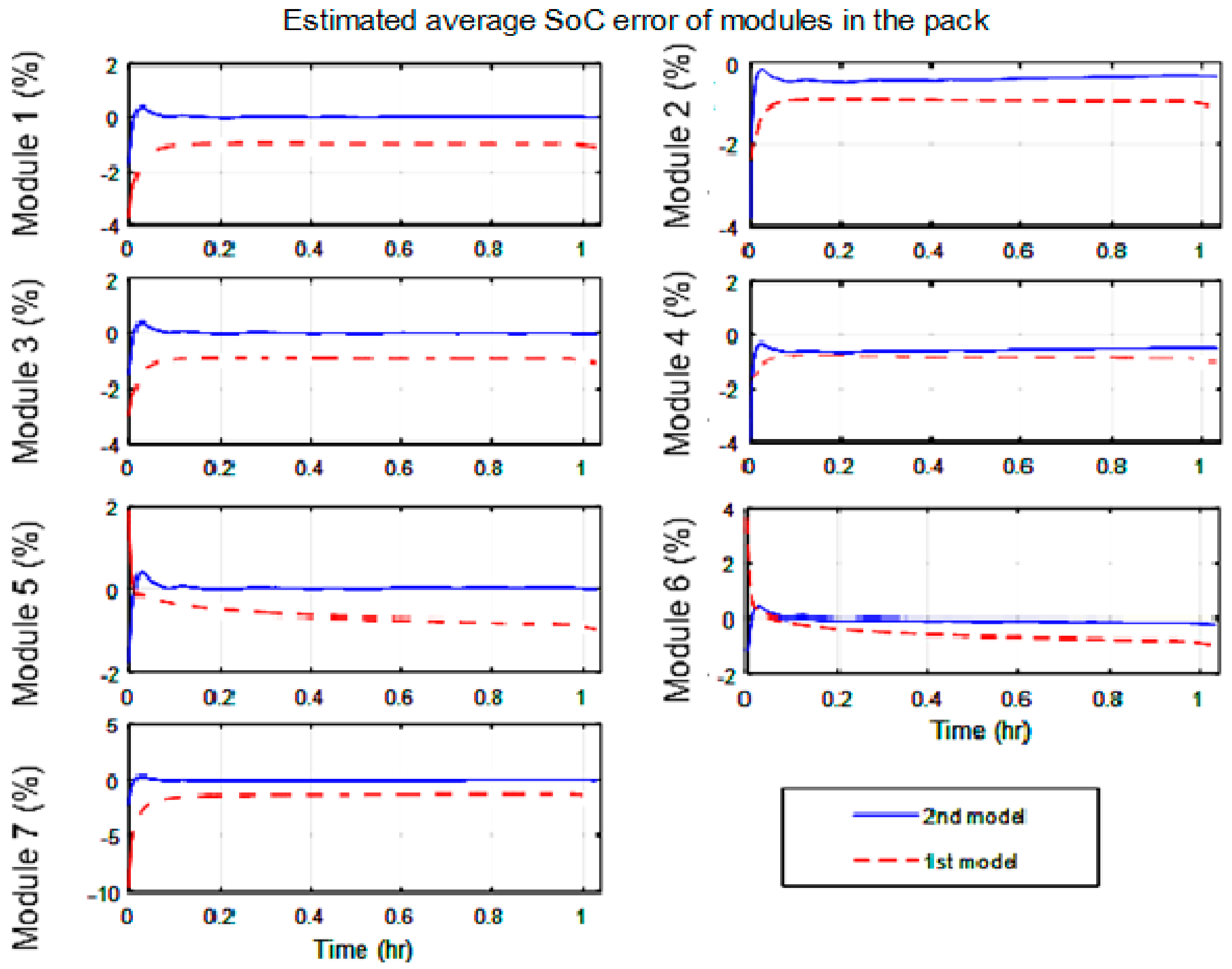
| The first order dynamic model | 1% | 1% | 1% | 1% | 1.2% | 0.9% | 2% |
| The second order dynamic model | 0.17 % | 0.4% | 0.15% | 0.5% | 0.17% | 0.02% | 0.17% |
References
- Zhou, Y.; Li, X. Overview of lithium-ion battery SOC estimation. In Proceedings of the 2015 IEEE International Conference on Information and Automation, Lijiang, China, 8–9 August 2015; pp. 2454–2459. [Google Scholar]
- Horiba, T. Lithium-Ion Battery Systems. Proc. IEEE 2014, 102, 939–950. [Google Scholar] [CrossRef]
- Xiong, R.; He, H. Cell State-of-Charge Estimation for the Multi-cell Series-connected Battery Pack with Model bIas Correction Approach. Energy Procedia 2014, 61, 172–175. [Google Scholar] [CrossRef][Green Version]
- Ng, K.S.; Moo, C.-S.; Chen, Y.-P.; Hsieh, Y.-C. Enhanced coulomb counting method for estimating state-of-charge and state-of-health of lithium-ion batteries. Appl. Energy 2009, 86, 1506–1511. [Google Scholar] [CrossRef]
- Zheng, Y.; Ouyang, M.; Han, X.; Lu, L.; Li, J. Investigating the error sources of the online state of charge estimation methods for lithium-ion batteries in electric vehicles. J. Power Sources 2018, 377, 161–188. [Google Scholar] [CrossRef]
- Thuy, N.V.; Van Chi, N. State of Charge Estimation for Lithium-Ion Battery Using Sigma-Point Kalman Filters Based on the Second Order Equivalent Circuit Model. In Lecture Notes in Networks and Systems 104, Proceedings of the International Conference on Engineering Research and Applications, ICERA 2019; Springer Nature Switzerland AG: Cham, Switzerland, 2020; pp. 664–678. [Google Scholar]
- Hu, X.; Li, S.; Peng, H. A comparative study of equivalent circuit models for Li-ion batteries. J. Power Sources 2012, 198, 359–367. [Google Scholar] [CrossRef]
- Yazdanpour, M.; Taheri, P.; Mansouri, A.; Schweitzer, B. A circuit-based approach for electro-thermal modeling of lithium-ion batteries. In Proceedings of the 2016 32nd Thermal Measurement, Modeling & Management Symposium (SEMI-THERM), San Jose, CA, USA, 14–17 March 2016; pp. 113–127. [Google Scholar]
- Xu, Y.; Hu, M.; Zhou, A.; Li, Y.; Li, S.; Fu, C.; Gong, C. State of charge estimation for lithium-ion batteries based on adaptive dual Kalman filter. Appl. Math. Model. 2020, 77, 1255–1272. [Google Scholar] [CrossRef]
- Ciortea, F.; Rusu, C.; Nemes, M.; Gatea, C. Extended Kalman Filter for state-of-charge estimation in electric vehicles battery packs. In Proceedings of the 2017 International Conference on Optimization of Electrical and Electronic Equipment (OPTIM) & 2017 Intl Aegean Conference on Electrical Machines and Power Electronics (ACEMP), Institute of Electrical and Electronics Engineers (IEEE). Brasov, Romania, 25–27 May 2017; pp. 611–616. [Google Scholar]
- Zhang, M.; Wang, K.; Zhou, Y.-T. Online State of Charge Estimation of Lithium-Ion Cells Using Particle Filter-Based Hybrid Filtering Approach. Complexity 2020, 2020, 1–10. [Google Scholar] [CrossRef]
- Tran, N.T.; Vilathgamuwa, D.M.; Li, Y.; Farrell, T.; Choi, S.S.; Teague, J. State of charge estimation of lithium ion batteries using an extended single particle model and sigma-point Kalman filter. In Proceedings of the 2017 IEEE Southern Power Electronics Conference (SPEC), Puerto Varas, Chile, 4–7 December 2017; pp. 1–6. [Google Scholar]
- Tong, S.; Lacap, J.H.; Park, J.W. Battery state of charge estimation using a load-classifying neural network. J. Energy Storage 2016, 7, 236–243. [Google Scholar] [CrossRef]
- Ben Sassi, H.; Errahimi, F.; Es-Sbai, N.; Alaoui, C. Comparative study of ANN/KF for on-board SOC estimation for vehicular applications. J. Energy Storage 2019, 25, 27. [Google Scholar] [CrossRef]
- Jiani, D.; Zhitao, L.; Youyi, W.; Changyun, W. A fuzzy logic-based model for Li-ion battery with SOC and temperature effect. In Proceedings of the 11th IEEE International Conference on Control & Automation (ICCA), Taichung, Taiwan, 18–20 June 2014; pp. 1333–1338. [Google Scholar]
- Wang, B.; Liu, Z.; Li, S.; Moura, S.J.; Peng, H. State-of-Charge Estimation for Lithium-Ion Batteries Based on a Nonlinear Fractional Model. IEEE Trans. Control. Syst. Technol. 2016, 25, 3–11. [Google Scholar] [CrossRef]
- Dai, H.; Wei, X.; Sun, Z.; Wang, J.; Gu, W. Online cell SOC estimation of Li-ion battery packs using a dual time-scale Kalman filtering for EV applications. Appl. Energy 2012, 95, 227–237. [Google Scholar] [CrossRef]
- Zhang, Z.; Cheng, X.; Lu, Z.-Y.; Gu, D.-J. SOC Estimation of Lithium-Ion Battery Pack Considering Balancing Current. IEEE Trans. Power Electron. 2017, 33, 2216–2226. [Google Scholar] [CrossRef]
- Van, C.N. State Estimation Based on Sigma Point Kalman Filter for Suspension System in Presence of Road Excitation Influenced by Velocity of the Car. J. Control. Sci. Eng. 2019, 2019, 1–16. [Google Scholar]
- Van Der Merwe, R. Sigma Point Kalman Filters for Probabilistic Inference in Dynamic State-Space Models. Ph.D. Thesis, OGI School of Science & Engineering, Oregon Health & Science University, Portland, OR, USA, 2004. [Google Scholar]
- Al-Shabi, M. Sigma-Point Filters in Robotic Applications. Intell. Control. Autom. 2015, 6, 168–183. [Google Scholar] [CrossRef]
- Tong, C.H.; Barfoot, T.D. A Comparison of the EKF, SPKF, and the Bayes Filter for Landmark-Based Localization. In Proceedings of the 2010 Canadian Conference on Computer and Robot Vision, Ottawa, ON, Canada, 31 May–2 June 2010; pp. 199–206. [Google Scholar]


| −5 °C | 5 °C | 15 °C | 25 °C | 35 °C | 45 °C | |
|---|---|---|---|---|---|---|
| 1.0870 | 0.9803 | 1.0221 | 1.0184 | 1.0543 | 1.0399 | |
| Q(mAh) | 2200 | 2200 | 2200 | 2200 | 2200 | 2200 |
| 250.0000 | 78.4916 | 63.6762 | 2.0749 | 170.0408 | 151.3064 | |
| 0.0073 | 0.0049 | 0.0048 | 0.0018 | 0.0036 | 0.0024 | |
| 0.0347 | 0.0257 | 0.0188 | 0.0177 | 0.0201 | 0.0185 | |
| 0.0013 | 0.0013 | 0.0012 | 0.0012 | 0.0012 | 0.0011 | |
| 0.6124 | 1.7556 | 0.3228 | 1.4882 | 0.2997 | 0.4631 | |
| 3.9035 | 7.5994 | 8.1119 | 36.8543 | 5.1841 | 6.5319 | |
| 0.0204 | 0.0203 | 0.0201 | 0.0019 | 0.0019 | 0.0019 | |
| 0.0494 | 0.0376 | 0.0288 | 0.0443 | 0.0136 | 0.0134 |
© 2020 by the authors. Licensee MDPI, Basel, Switzerland. This article is an open access article distributed under the terms and conditions of the Creative Commons Attribution (CC BY) license (http://creativecommons.org/licenses/by/4.0/).
Share and Cite
Nguyen Van, C.; Nguyen Vinh, T. Soc Estimation of the Lithium-Ion Battery Pack using a Sigma Point Kalman Filter Based on a Cell’s Second Order Dynamic Model. Appl. Sci. 2020, 10, 1896. https://doi.org/10.3390/app10051896
Nguyen Van C, Nguyen Vinh T. Soc Estimation of the Lithium-Ion Battery Pack using a Sigma Point Kalman Filter Based on a Cell’s Second Order Dynamic Model. Applied Sciences. 2020; 10(5):1896. https://doi.org/10.3390/app10051896
Chicago/Turabian StyleNguyen Van, Chi, and Thuy Nguyen Vinh. 2020. "Soc Estimation of the Lithium-Ion Battery Pack using a Sigma Point Kalman Filter Based on a Cell’s Second Order Dynamic Model" Applied Sciences 10, no. 5: 1896. https://doi.org/10.3390/app10051896
APA StyleNguyen Van, C., & Nguyen Vinh, T. (2020). Soc Estimation of the Lithium-Ion Battery Pack using a Sigma Point Kalman Filter Based on a Cell’s Second Order Dynamic Model. Applied Sciences, 10(5), 1896. https://doi.org/10.3390/app10051896