Article

Graphs Regularized Robust Matrix Factorization and Its Application on Student Grade Prediction

School of Computer Science, Northwestern Polytechnical University, Xi’an 710129, Shaanxi, China
*
Author to whom correspondence should be addressed.
Appl. Sci. 2020, 10(5), 1755; https://doi.org/10.3390/app10051755
Submission received: 9 January 2020 / Revised: 18 February 2020 / Accepted: 21 February 2020 / Published: 4 March 2020
(This article belongs to the Special Issue Applied Machine Learning)

Abstract

:
Student grade prediction (SGP) is an important educational problem for designing personalized strategies of teaching and learning. Many studies adopt the technique of matrix factorization (MF). However, their methods often focus on the grade records regardless of the side information, such as backgrounds and relationships. To this end, in this paper, we propose a new MF method, called graph regularized robust matrix factorization (GRMF), based on the recent robust MF version. GRMF integrates two side graphs built on the side data of students and courses into the objective of robust low-rank MF. As a result, the learned features of students and courses can grasp more priors from educational situations to achieve higher grade prediction results. The resulting objective problem can be effectively optimized by the Majorization Minimization (MM) algorithm. In addition, GRMF not only can yield the specific features for the education domain but can also deal with the case of missing, noisy, and corruptive data. To verify our method, we test GRMF on two public data sets for rating prediction and image recovery. Finally, we apply GRMF to educational data from our university, which is composed of 1325 students and 832 courses. The extensive experimental results manifestly show that GRMF is robust to various data problem and achieves more effective features in comparison with other methods. Moreover, GRMF also delivers higher prediction accuracy than other methods on our educational data set. This technique can facilitate personalized teaching and learning in higher education.

1. Introduction

In high school education, student grade prediction (SGP) can make great sense for aiding all stakeholders in the education process. For students, SGP can help them to choose suitable courses or exercises for increasing their knowledge, and even to make their pre-plans for academic periods. For instructors, SGP can help them to adjust learning materials and teaching programs based on student ability, and to find the students that are at risk of disqualification in course progress. For educational managers, SGP can help them to check the curriculum program and to arrange the courses in a scientific order. All stakeholders of the educational process could have a better self-plan to improve education outcomes and then have a higher graduation rate. SGP is an important problem for scientific education in STEM (Science, Technology, Engineering, Mathematics), referred to in the work of G. Shannon et al. [1].
Student grade prediction aims to predict the final score/grade of course enrolled by a target student in the next academic term. SGP provides a useful reference to evaluate educational outputs in advance and is thus significant necessary for various tasks towards personalized education, such as ensuring on-time graduation [2] and improving learning grade [3,4]. Over the past years, many studies have paid attention to SGP and have already developed many methods [5].
Existing methods can be principally divided into three categories depending on their formulation, as follows: (1) Classification problem. SGP is recast as labeling the target student with the predefined grade tags and was solved by classification models, such as decision tree [6], logic regression [7,8] and support vector machine [9,10]. (2) Regression problem. By taking the grade as the response variable, SGP is rewritten into assigning scores following the features of student or course, such as linear regression [5,11,12], neural network [13,14,15] and random forest [9]. (3) Matrix completion. Since grade records can be poured into a matrix, SGP is also formulated as predicting the missing values of the student-course matrix with each element being a course grade [16]. This formulation is usually solved by the popular method of matrix factorization and has been extensively studied, leading to many effective approaches [17,18]. In particular, based on the same dataset, Thai-Nghe et al. compared matrix competition with traditional regression methods such as logistic/linear regression and the experimental results show that matrix competition can improve prediction results [19].
MF based methods aim to learn the latent features of student and course from the given grade data and then uses these features for SGP [20]. Here, we review the related works that using MF techniques. Traditional MF was employed to implicitly encode “slip rate” (the probability that the student knows how to solve a question but makes a mistake) and the “guess rate” (the probability that the student does not know how to solve a question but guesses correctly) of the student in an examination, resulting in an excellent performance on the educational data set of KDD (Knowledge Discovery and Data Mining) Cup 2010 [21]. In References [22,23], Non-negative Matrix Factorization (NMF) was used to integrate the nonnegativity of student grade. Tensor factorization (TF) was exploited to take the temporal effects into account in Reference [24], due to the improvement of the ability of students. Since grade matrix is implicitly low rank, low-rank matrix factorization (LRMF) was investigated in data sets from the online learning platform in the work of Lorenzen et al. [25]. But the existing MF based methods often suffer from the issues of missing data, corrupted data, and data noise. Especially, they fail to consider the side information which is included in the other handy educational data, such as background data and daily behavior data in school.
Since the L 2 -norm based reconstruction is sensitive to outliers and data corruptions, Lin et al. proposes to use L 1 -norm instead of L 2 -norm to enhance the robustness [26,27,28]. Besides, we often have massively available side information data in real-world applications. Rao et al. proposes a method of graph regularized alternating least squares (GRALS) to integrated two graphs from the side information data of movies and viewers [29]. More specifically, in the real context of high education, the data set usually has the following properties: (1) The grade matrix is heavily lost for course selection and corrupted by some human factors. (2) The students with similar backgrounds are likely to have similar performance in a course [30]. For example, two students both have more exercises in computer programming, and then they may both obtain a perfect grade at their course of C language with a high probability. (3) The courses with similar knowledge tend to give rise to a similar grade for a student. For instance, C Language is similar with Data Structure while C Language is not similar with History, thus student who is good at C Language is likely to have good performance in Data Structure but not necessarily History.
To this end, we put forth a novel MF method, called double graph regularized robust matrix factorization (GRMF), following by applying GRMF for SGP as shown in Figure 1. GRMF not only uses the robust loss function from RMF-MM but also integrates two side information graphs constructed using the background data of students and courses. The MM algorithm can effectively solve the resulting optimization problem. Two-folds contributions of our paper are summarized as follows:
  • We propose a new model of matrix factorization, dubbed Graph regularized Robust Matrix Factorization (GRMF), by considering both the robustness to data pollution and the side information from background descriptions.
  • We design a workflow by applying GRMF on the problem of SGP, shown in Figure 1, where the real-world data set is collected from our university.
The rest of this paper is organized as follows—in Section 2, we formulate the problem of SGP, followed by brief reviewing the MF technique. We present GRMF in Section 3 and the GRMF algorithm in Section 4. Section 5 shows the experimental results on movie rate prediction, image recovery, and SGP. Section 6 finally concludes this paper.

2. Ralated Works

In this section, we formulate the problem of SGP in the form of mathematics, followed by introducing the promising technique of matrix factorization.

2.1. Student Grade Prediction (SGP)

In current higher education in university, the teachers provide a “one-size-fits-all” curriculum, while the students enroll many courses to obtain academic credit. To graduate on time, the student expects to know which course he/she can pass with high score/grade, while the teacher expects to know which student has a risk of failure in his/her course. Hence, the problem of predicting the student grade at a course is significant to improve the educational outcomes.
Generally speaking, the grade of one student at a target course can be inferred by his/her learning records, including historical grades in enrolled courses, academic behaviors and his/her background [31,32]. In this paper, we make the following assumption—the grade can be determined by the latent features of student and course, where those features can be derived from the data of students and courses. We explicitly define the task of SGP as follows:
Problem 1 (Student Grade Prediction): Let g ( s , c ) be the grade of student s at course c. Denote by u s the feature of student s and v c the feature of course c. Given the grade matrix M , SGP aims to seek the mapping H ( u s , v c ) , such that g ( s , c ) = H ( u s , v c ) for all grades in M .
To solve Problem 1, we should extract u and v and design a mapping using the given data matrix M . Most research designs or learns the features by using the background information [33,34], such as student age and credit time, or the student grades on all finished courses. Since both of them are helpful, in this paper, we combine both information for SGP through developing the MF [26].

2.2. Matrix Factorization

Letting M R m × n be the given matrix, MF aims to seek two latent feature matrices U R m × k and V R m × k to approximate M. The traditional MF can be written as:
min U , V | | M U V T | | F ,
where k is the number of latent features predefined in U and V, and | | · | | F is the Frobenius norm. Optimization problem (1) can be solved by various algorithms, such as Majorization Minimization (MM) [35], alternating the direction of the method of multipliers (ADMM) [36], simulated annealing (SA) [37]. Besides, many variants of MF have been proposed, including LRMF [25], NMF [22] and TF [24].
To enhance the robustness, robust matrix factorization via majorization minimization (RMF-MM) employs L 1 -norm instead of L F -norm as the reconstruction term [26]. The objective problem of RMF-MM is:
min U , V | | W M U V T | | 1 + λ 2 | | U | | F 2 + λ 2 | | V | | F 2 ,
where | | · | | 1 is L 1 -norm of matrix, λ > 0 is a regularization parameter and W is defined as follows:
W i j = 0 , the value of M i j is missing 1 , o t h e r w i s e .
The problem above can be effectively optimized by MM algorithm. The results in the experiments by Lin et al. show that RMF-MM is robust to high missing rate or severe data corruption [26].
Since RMF-MM can effectively learn the features from noisy data and then uses the features for prediction, we reformulate the Problem 1 for employing this novel technique, as follows:
Problem 2. (SGP-MF): Given a student grade matrix M , SGP-MF aims to extract U for students and V for courses such that M = UV . Then the target grade is predicted by
g ( s , c ) = M s , c = u s T v c ,
where g ( s , c ) is the grade of student s on course c, u s is the s-th row of U and v c is the c-th row of V . And M s , c is the element of s-th row, c-th column of matrix M .
The reason we consider the Formula (4) is the fact that a student enrolls on a course and obtains a grade. This fact motivates us to obtain the student’s features and course’s features, given the grade matrix. In this paper, we consider this problem using the matrix factorization (MF) method. As in Formula (4), each grade M s , c is made by u s T v c to obtain the latent features
However, RMF-MM fails to consider the side-information data that is often available. The method of graph matrix factorization (GMF) is an approach to integrate the neighborhood structure of M , but it does not work for matrix completion [38]. Based on GMF, we here solve the SGP by combining two side information graphs with RMF-MM.

3. Double Graph Regularized Robust Matrix Factorization

In this section, we present our motivation for considering side information data in SGP and encode them into two graphs, followed by our objective problem and its detail optimization with MM.

3.1. Motivation

In real-world education, various related information can be obtained from the student, such as background, daily life, and student behaviors, as well as course. These side information data contain the relationships among students and courses that can be used for enhancing the prediction performance. Hence, we in this paper propose to encode them in two graphs, followed by integrating them into RMF.
More specifically, we list some observations: (1) The family background, such as the economic situation and educational level of their parents, influences the scope of student knowledge [39]. (2) The background of students, such as majors and ages, may affect their habits of thinking and learning. (3) The related course contains much overlapping knowledge or similar skills. (4) Courses taught by an identical teacher are similar in the style of teaching and testing [40].
From the above observations, we have the follows: On the one hand, it is believed that students with a similar background can obtain similar performance. On the other hand, two similar courses tend to have similar grade distribution.

3.2. Side Information Graph

Considering the row/column vectors of M as data points, each row vector of U / V is the low-rank representation of the corresponding row/column in M . Note that each row in both M and U corresponds to a student, while each column in both M and V T corresponds to a course. Besides, we have side information feature matrixes from students and courses, denoted by S u and S v . Following above, if two students/courses are close in terms of S u / S v , then the corresponding rows of U / V are also close to each other [41,42].
In order to simultaneously integrate the side information of students and courses, we knit two similarity graphs using S u and S v instead of using M [38,43,44]. That is the reason that the graphs here are called side information graph. The method of building graph is as follows. Denote by Q = { S , E | G } the side information graph, where S includes all data points from students or courses, E is the set of edges, and G contains all weights on all edges. G is constructed by:
G i j = e | | s i s j | | 2 σ , s i N k s j or s j N k s i 0 , otherwise ,
where s i is corresponding to the data point in S u or S v , σ is the kernel parameter and N k { x } indicates the set of k neighbors to sample x . The details can be found in the literature [41].
Since the similarity relationships encoded in the side information graphs are constructive for learning the latent features, we hope to preserve them in U and V . Taking U for example, we, as usual, employ the following objective [41]:
R 1 = 1 2 i , j G i , j | | u i u j | | 2 2 = t r U T H u U ,
where t r ( · ) denotes the trace of a matrix, u i is the row of U and H u = D G , D i i = j G i , j . Similarly, we can knit the side information graph of course and then obtain two Laplacian regularization terms.

3.3. The Objective Problem of GRMF

With the idea of integrating the side information, we combine the objective of RMF-MM and the two Laplacian regularizations, as follows:
min U , V | | W ( M U V T ) | | 1 + λ 2 | | U | | F + | | V | | F + α 2 t r U T H u U + t r V T H v V ,
where λ > 0 , α 0 are two trade-off parameters, and H u / H v is defined in the above section. From (7), we can believe that GRMF can reach a better performance than RMF-MM, since GRMF degenerates into RMF-MM when α is zero.
The main difference between GRMF and RMF-MM lies in the graph Laplacian regularizers of (6), where GRMF integrates more data priors. While GRALS uses L 2 -norm for data fidelity [29]. GRMF proposes to adopt L 1 -norm and thus is more robust to data noise and pollution.
The SGP problem is first described as a machine learning problem, shown in Problem 1. We assume the grade is determined by the student’s latent features and the course’s latent features. This assumption is general. The problem is then reformulated by matrix factorization (MF), since we plan to adopt MF to learn the latent features. In order to consider the noise in the given grade matrix, we reformulated the objective of MF by L 1 normal, because the noise is considered from the grade temper, slipping, and so forth. Finally, for better prediction result, we consider the relationship of students and the relationship of courses in our robust MF model though two graph regularization items. Our objective is thus shown in Equation (7).

4. GRMF Algorithm

In this section, we use a majorization-minimization algorithm to solve problem (7). Suppose that we already have obtained ( U k , V k ) after the k-th iterations. We split ( U , V ) as the sum of ( U k , V k ) and the unknown residue ( Δ U k , Δ V k ) :
( U k + 1 , V k + 1 ) = ( U k , U k ) + ( Δ U k , Δ V k ) .
The task can now be finding the small increment ( Δ U k , Δ V k ) in the k-th iteration such that the objective function keeps decreasing. To seek the best ( Δ U k , Δ V k ) , we employ the linearized Direction Method with Parallel Splitting and Adaptive Penalty (LADMPSAP) [45]. We made the detailed procedure of this optimization in Appendix A. We summarize the main flow of GRMF to make the paper self-contained in Algorithm 1, shown as below:
Algorithm 1: Graph regularized Robust Matrix Factorization (GRMF) by Majorization Minimization
Input: M R n × m , α , and λ
Output: U and V
Method:
  Initialize U 0 and V 0 with using SVD on M;
   Δ U 0 = Δ V 0 = 0 ; ε 1 = ε 2 = 1 e 6 .
  While not converged when we arrived ( U k , V k ) , do
      Let t = 1;
      While not converged, do
            Update Δ U t and Δ V t via LADMPSAP;
            t = t + 1;
      End while
       ( Δ U k , Δ V k ) = ( Δ U t , Δ V t ) ;
      Update U and V in parallel:
             U k + 1 = U k + Δ U k ;
             V k + 1 = V k + Δ V k ;
      Check the convergence coditions, if
             V k + 1 V k < ε 1 and U k + 1 U k < ε 2 ;
End while.

5. Experimental Results

In order to evaluate the performance of GRMF, we conducted the following experiments: (1) testing GRMF, RMF-MM and on MOVIELENS 100k datasets and a public image data; (2) comparing GRMF with several fashion methods for student grade prediction, including RMF-MM [26], GRALS [29], MF [46], NMF [22], PMF [47], KNN(k-Nearest Neighbor) [48] and column mean [49] using the real educational dataset from our university. Note that MF is the standard matrix factorization solved with gradient descent; column-mean is the mean scores of historical grades of target course; and for KNN-mean, we obtained the k neighbor students and then computed the grade mean. The code and data sets are available on our website, https://github.com/ypzhaang/student-performance-prediction.

5.1. Evaluation Metric

Three metrics are used for evaluating the results: Root Mean Squared Error (RMSE), L 1 -norm Error (Err1) [26], PSNR (Peak Signal to Noise Ratio) and Acc (Accuracy rate). Especially, in our paper, Acc is computed as follows:
A c c = i = 1 n Δ g i n ,
where
Δ g = 1 , | g r e g | 0.5 0 , | g r e g | < 0.5 ,
in which g r e is the predicted grade while g is the true grade and n is the number of grades.

5.2. Test on a Toy Data from Movie Dataset

MovieLens data sets were collected by the GroupLens Research Project at the University of Minnesota. These data sets consist of 100,000 ratings (1–5) from 943 users on 1682 movies, background information from users (e.g., age, occupation, and zip code) and movies (e.g., title, release date, and genre). Besides, users who have less than 20 ratings or do not have completed demographic information were removed. In this test experiment, we draw out a toy data set from MovieLens to probe the effectiveness, convergence, and parameter effects of GRMF. And in the toy data set, the user ids are less than 200, and the movie ids are less than 300.

5.2.1. Rating Prediction and Algorithm Convergence

We divided the toy data set into a training set and test set by random sampling. To evaluate the small toy data, we employed a five-fold cross validation that trains models on four-fold samples and tests on the remaining samples. Whereby we constructed two five-nearest neighborhood graphs from the background data of both users and movies. We chose suitable parameters for achieving best performance using all the mentioned methods. Note that the optimal parameters of GRALS were selected in Reference [29].
Table 1 shows the prediction results from using four methods on the toy data set. It is easy to observe that: (1) MF is better than RMF-MM and GRALS in terms of RMSE, but worse than the two latter compared to Err1. (2) RMF-MM has better performance on Err1 than GRALS, which is more robust to evaluate. (3) Overall, our method delivers the best results using either RMSE or Err1. All the above says that GRMF can benefit from the side information data to enhance rate prediction performance.
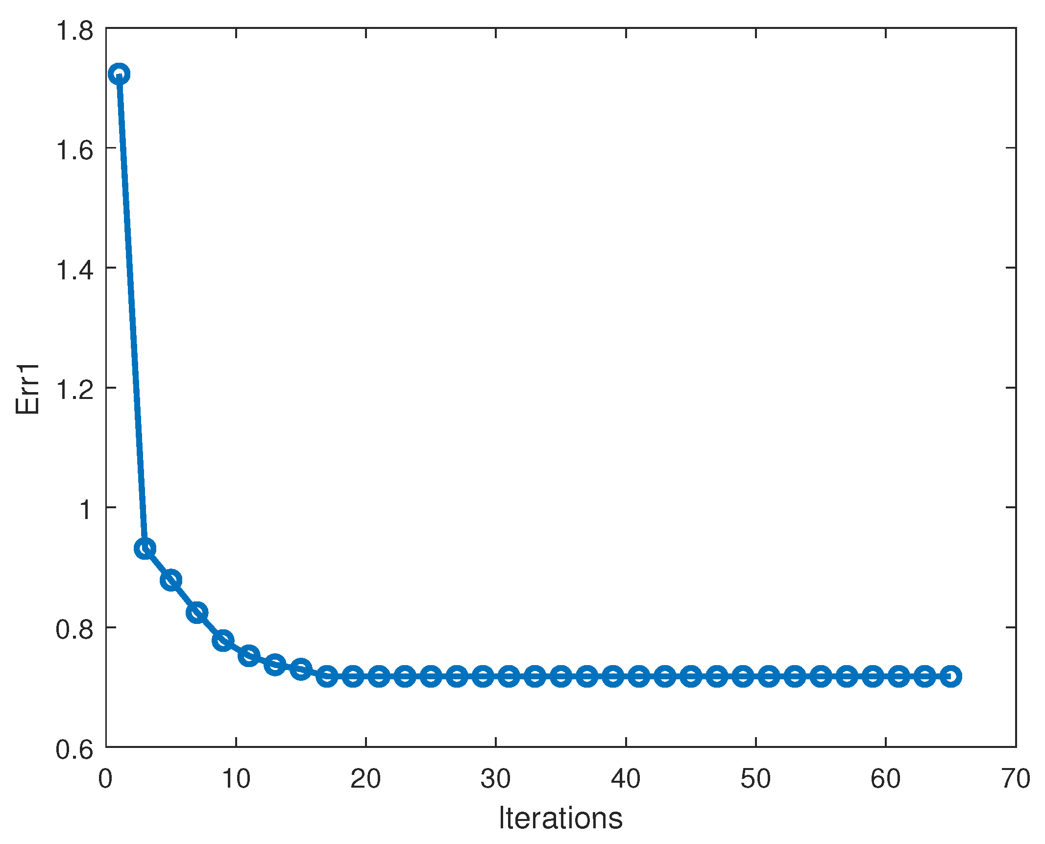
In addition, Figure 2 displays the convergence proceeding of GRMF on the toy data. As is shown, GRMF can converge to stable Err1 after about 16 iterations. With more observations on other data sets, Algorithm 1 can have a fast convergence and arrive at an effective solution.

5.2.2. The Effects of Parameters on Rating Prediction

We have the graph regularization parameter α , the regularization parameter λ and the rank of factorized matrices k in the objective (7) of GRMF. We here discuss the effects of these three parameters on the prediction performance utilizing the above toy data set on our prediction experiment.
The two parameters of α and λ vary in wide ranges as is shown in Figure 3b. Figure 3b shows the 3D curve of Err1 created under the effects of α and λ . From the curve, we observe that there is a broad range of parameter pairs that can be available for producing decent prediction results. Besides, we also probe the effect of the parameter k, shown in Figure 3a. The results show that GRMF has the most stable performance under varying k, while the RMF-MM has the worst performance.

5.3. Evaluation on Image Data Set

The problem of image recovery is often formulated as matrix completion. Since the top singular values dominate the main information, most of the images could be regarded as a low-rank matrix. Hence, we apply the proposed method to recover the image from its noisy version. This test aims to recast the experiment conducted in the work of Lin et al. [26]. Concretely, we pollute the images (https://sites.google.com/site/zjuyaohu/) with Gaussian noise or salt-and-pepper noise, then recover the images from the noisy version in comparison with the methods of RMF-MM and GRALS.

5.3.1. Gaussian Noise

We added Gaussian noise with the variance being 1 and mean being 0 to g percent of the observed pixels, where g is the corruption ratio. Figure 4b shows the example image which was corrupted with Gaussian noise. g was varied in the range of [45, 90] to observe the performance in various situations. We ran the three methods to recover the corrupted image in Figure 4b, where the side-information data consists of the rows and columns of the corrupted image. Figure 5 shows the PNSRs (Peak Signal to Noise Ratios) from the three compared methods. From the curves, GRMF consistently achieves the highest PSNRs on all test cases. When the corruption ratio increases, GRMF delivers a much better result than RMF-MM. Note that GRALS has a weak performance because its reconstruction term is very sensitive to data pollutions.
Figure 4c–e depicts the resultant images from the case of g = 80, using the three methods. As is clear, our GRMF produces the best visualization, while the other methods suffer a few horizontal or vertical lines.

5.3.2. Salt-And-Pepper Noise

We added the salt-and-pepper noise with noise density varying from 0.05 to 0.65 with a step of 0.05 to image and obtained the corrupted image, like Figure 6b. Then, we ran the three compared methods for denoising the corrupted image where the side-information consists of the rows and the columns of the corrupted image. Figure 7 shows the results of image denoising by GRALS, RMF-MM, and GRMF. From Figure 7 it is clear that GRMF delivers the best performance on PSNR when the noise density is less than 0.4 but drops down if the noise density is greater than 0.5, where the other two methods obtained worse results. The reason is that most pixels of the image are corrupted so that the graphs are difficult to obtain well in a noisy situation. In addition, Figure 6 shows the resultant images when the noise density is 0.4, where our method touches the highest PNSR of 22.88 dB.

5.4. Application on Educational Data Set

The data were collected from the school of Computer Science, Northwestern Polytechnical University (NPU), across students who joined in the past five years, that is, from 2013 to 2017. We collected all the score/grade recorders before the fall of 2017, together with the side information.
More specifically, our dataset contains the grades, the side data of student and the side data of courses, respectively denoted by NPU-G, NPU-S, and NPU-C for short. NPU-G is composed of 1325 × 832 grade records from 1325 students at 832 courses. NPU-S contains 25 description features of 1325 students, such as ages, gender, and department. NPU-C includes 18 description features of 882 academic/elective courses, such as hours, type, and course credit. In addition, at least 15 students enrolled and obtained grades in each course, and students starting university in 2013 and 2014 have already completed their program.
SGP in our educational data set has the following challenges: (1) Data sparsity. There are 832 courses in NPU-G, but each student is only required to enroll in a small number of courses, i.e., about 85 courses in our data. (2) data corruption. Many subjective factors affect the final grade, e.g., subjective questions. (3) missing data. A few students do not attend the final exam, and thus give an empty grade in the information system. All this noisy information makes our problem very challenging.

5.4.1. Educational Data Preprocessing

For NPU-G, we removed the students who had lost most of the data records or had taken less than 4 courses, and then removed those courses that were taken by less than 15 students, followed by deleting the secondary courses to ensure a single record per student. Finally, we formulated the remaining records from 882 students and 82 courses into the matrix M , ordered by scholar terms. In addition, we transformed the scores into grade 1–6 using the following piecewise function:
y = 1 0 < x < 60 ; 2 60 x < 70 ; 3 70 x < 80 ; 4 80 x < 90 ; 5 90 x < 100 ; 6 x = 100 .
where x is the score in the grade record while y is its corresponding grade.
Responding to M R 882 × 15 , we also removed the student and the course from NPU-S and NPU-C. In all collected side descriptions, we selected 15 and 12 important features for NPU-S and NPU-C, respectively, using teaching experience. Finally, we formulated them into matrices S u R 882 × 15 for students and S v R 82 × 12 for courses.

5.4.2. Implementation Details

We here predict the student grade for each academic term, because of the usual stages at the university. Hence, we used historical records as a training set to predict the grade in the next term. That is, our model was trained on the records from the 1-th to the (t − 1)-th terms and was tested on the t-th terms. Concretely, in the SGP tasks for the t-th term, we built k-nearest neighborhood graph G u / G v on the side data of students and courses S u / S v , respectively. Then, we learned the latent features of student and course on training data using our model, followed by computing the evaluation matrix Err1 and Acc. We conduct this experiment on six data splits, where the sizes of training sets and test sets are listed in Table 2.
In order to compare with other methods for SGP, we conducted an experiment using MF (S. Rendle, 2010 [46]), NMF (C.S. Hwang, et al., 2015 [22]), PMF (B. Jiang, et al. [47]), KNN ( N.C. Wong, et al., 2019 [48]) and column mean (M. Sweeney, et al. [49]). Besides, we also implement SGP using RMF-MM (Z. Lin, et al., 2018 [26]) and GRALS(N. Rao, et al. [29]). For each method, we selected the optimal one from the wide range suggested by their related reports.

5.4.3. Experimental Result and Discussion

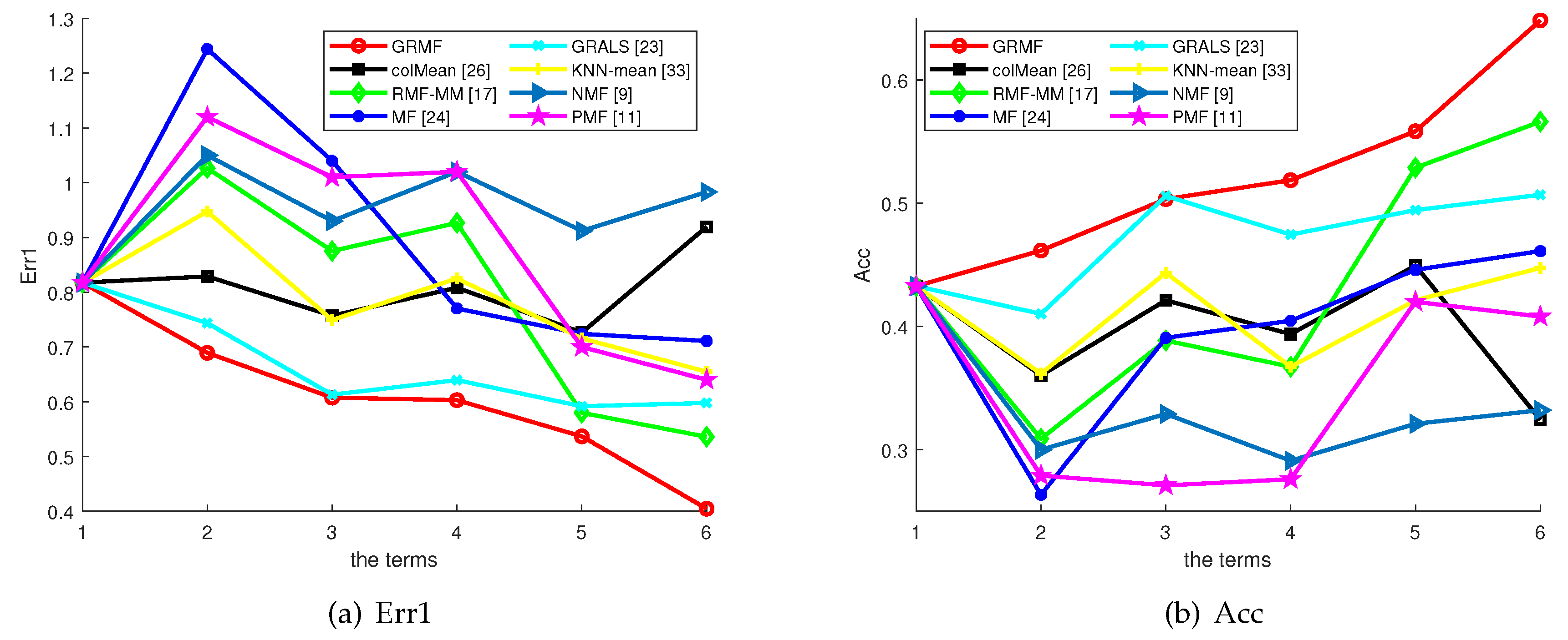
Figure 8a and Figure 8b show the prediction results from varying all six terms by various methods in terms of Err1 and Acc. From the curves and comparisons, we observe that: (1) as the semester progresses, the prediction decreases in Err1 and increases in accuracy rate; (2) both GRMF and GRALS are better than other comparable methods; (3) GRMF is not only better than RMF but also outperforms GRALS. (4) the prediction performance of colMean can be regarded as a base performance of SGP. Both GRMF and GRALS can perform better than colMean over all the terms while other methods, including the RMF-MM performance are worse than colmean in most cases.
From these observations, we derive the following conclusions: (1) As the semester progresses, we obtain more information about the student/course which is reflected in the better prediction performance. (2) Side information data of student and course is helpful for SGP. (3) The combination of the side information and the robust L 1 regularizers in our methods GRMF improves the prediction performance effectively. (4) The methods using side information do perform well but other comparable methods cannot handle the prediction task well in the real education context due to the complex problem of real educational data. (5) Our proposed method outperforms traditional classification methods and regression methods. (6) The proposed method GRMF can achieve the accuracy of 65.4% in the sixth term, which is more interesting than the other methods.

6. Discussion and Conclusions

In this paper, we solve the student grade prediction (SGP) problem by proposing a novel matrix factorization method that is dubbed GRMF. GRMF integrates the side information with the robust objective function of matrix factorization, which can be effectively solved by the MM optimization algorithm. The extensive experiments are conducted on movie data, image data, and our education data for testing the performance on rate prediction, image recovery, and SGP. The evaluation results by the used matrices show that GRMF can deliver a better performance than all compared methods. In SGP, GRMF can achieve the highest accuracy of about 65.4 % . However, it is still weak in our challenging data. We will improve GRMF and try other fashionable methods to pursue a higher accuracy, while boosting a personalized education.
In addition, a function f that maps from U and V to the grade matrix G could be used to achieve a better prediction model, due to the gap between the predicted grade and the real grade. That is because the noise is often caused by accidental events, like exam slipping and guessing. Our study has this limitation on considering this noise in grade prediction. Adding this map f may help to obtain more accurate results in the real-world environment. We leave this study for future work.

Author Contributions

Conceptualization, Y.Z. and Y.Y.; Data curation, Y.Y. and J.C.; Formal analysis, Y.Z.; Funding acquisition, Y.Z. and X.S.; Investigation, Y.Y. and H.D.; Methodology, Y.Z.; Resources, J.C. and X.S.; Software, Y.Z. and Y.Y.; Supervision, X.S.; Validation, H.D. and J.C.; Writing—original draft, Y.Z. and Y.Y.; Writing—review & editing, H.D., J.C. and X.S. All authors have read and agreed to the published version of the manuscript.

Funding

This research was funded by the National Natural Science Foundation of China (Grants No. 61802313, 61772426, U1811262) and the Fundamental Research Funds for Central Universities (Grant No. G2018KY0301).

Acknowledgments

We thank the editors and any reviewers for their helpful comments.

Conflicts of Interest

The authors declare no conflict of interest.

Appendix A. Objective Minimization

Suppose that we already have obtained ( U k , V k ) after the kth iterations. We split ( U , V ) as the sum of ( U k , U k ) and the unknown residue ( Δ U , Δ V ) .
( U , V ) = ( U k , U k ) + ( Δ U , Δ V )
In a similar way, the graph regularization of (6) can be rewritten as follows:
L ( Δ U , Δ V ) = t r U T + Δ U T H u U + Δ U t r V T Δ V T H v V + Δ V
With (7) and (8), our task is to minimize the following:
min Δ U , Δ V H k Δ U , Δ V = min Δ U , Δ V W M U k + Δ U V k T + Δ V T 1 + λ 2 U + Δ U F 2 + V + Δ V F 2 + α 2 L ( Δ U , Δ V )
Now our task is to find a small increment ( Δ U , Δ V ) such that the objective function keeps decreasing. Inspired by [26], we try to relax (9) to a convex surrogate.
By using the triangular inequality of norms, we arrive at the following inequality:
H k Δ U , Δ V W M U k V k T Δ U V k T U k Δ V T 1 + λ 2 U + Δ U F 2 + V + Δ V F 2 + α 2 L Δ U , Δ V + W Δ U Δ V T 1 .
Besides, we can introduce the following relaxation:
W Δ U Δ V T 1 1 2 Λ u Δ U F 2 + 1 2 Λ v Δ V F 2 .
For simplicity, we define J k Δ U , Δ V as follows:
J k Δ U , Δ V = W M U k V k T Δ U V k T U k Δ V T 1 + λ 2 U + Δ U F 2 + V + Δ V F 2 + α 2 L ( Δ U , Δ V ) .
Then we have the relaxed function of H k Δ U , Δ V . Our optimization problem can be recast as:
F k Δ U , Δ V = J k Δ U , Δ V + 1 2 Λ u Δ U F 2 + 1 2 Λ v Δ V F 2 .
Thus, our optimization problem (9) can be further rewritten as:
min E , Δ U , Δ V W E 1 + ( λ 2 U + Δ U F 2 + 1 2 Λ u Δ U F 2 ) + ( λ 2 V + Δ V F 2 + 1 2 Λ v Δ V F 2 ) + α 2 L ( Δ U , Δ V ) s . t . M U k V k T = E + Δ U V k T + U k Δ V T ,
where Λ u , Λ v are diagonal matrices.
We optimize the objective by the Linearized Alternating Direction Method with Parallel Splitting and Adaptive Penalty (LADMPSAP) [45], as follows.

Appendix A.1. Updating E

Fixing other variables, updating E is equivalent to the following problem:
min E W E 1 + E E i + Y ^ i / δ e ( i ) F 2 .
where
Y ^ i = Y i + β i ( E i + Δ U i V k T + U k Δ V i T M + U k V k T ) ,
and δ e ( i ) = η e β i , η e = 3 L e + ε , where 3 is the number of variables which have to be updated in parallel, such as E , Δ U i , and Δ V i . Specially, L e is the squared spectral norm of the linear mapping on E , which is equal to 1, and ε is a small positive scalar. Then we update E by:
E i + 1 = W S σ e ( i ) ( E i Y ^ i / δ e ( i ) ) + w ¯ ( E i Y ^ i / δ e ( i ) ) ,
where S is the shrinkage operator [50]:
S ε x = m a x ( | x | ε , 0 ) s g n ( x ) ,
where w ¯ is the complement of W .

Appendix A.2. Updating ΔU

Updating Δ U is to solve the following problem:
min Δ U λ 2 U k + Δ U F 2 + α 2 t r ( ( U k T + Δ U T ) H u ( U k + Δ U ) ) + 1 2 Λ u Δ U F 2 ) + δ u ( i ) 2 Δ U Δ U i + Y ^ i V k / δ u ( i ) F 2
where δ u ( i ) = η u β i and η u = 3 V k 2 2 + ε . Since all terms in (A13) is convex, (A13) is a convex problem and its closed solution can be obtained by:
Δ U i + 1 = ( λ I m + α H u + Λ u T Λ u + δ u i I m ) 1 ( λ U k α U k H u + δ u ( i ) Δ U i δ u ( i ) Y ^ i V k / δ u ( i ) ) ,
where m can be found in the paper [26].

Appendix A.3. Updating ΔV

Similar to Δ U , updating Δ V can be achieved by:
Δ V i + 1 = ( λ I m + α H v + Λ v T Λ v + δ v i I m ) 1 ( λ V k α V k H v + δ v ( i ) Δ V i δ v ( i ) Y ^ i U k / δ v ( i ) ) .

Appendix A.4. Updating Y and β

We update Y and β as follows:
Y i + 1 = Y i + β i ( E i + 1 + Δ U i + 1 V k T + U k Δ V ( i + 1 ) T U k V k T M ) ,
β i + 1 = m i n ( β m a x , ρ β i ) ,
where ρ is defined by:
ρ = ρ 0 , i f Q < ε 1 1 , o t h e r w i s e ,
and
Q = β i m a x ( η e | | E i + 1 E i | | F , η u | | Δ U i + 1 Δ U i | | F , η v | | Δ V i + 1 Δ V i | | F ) / | | M U k V k T | | F .
In addition, the stopping criterion of iteration can be derived from KKT condition [45]:
β i max ( η e | | E i + 1 E i | | F , η u | | Δ U i + 1 Δ U i | | F , η v | | Δ V i + 1 Δ V i | | F ) / | | M U k V k T | | F < ε 1 ,
| | E i + 1 Δ U i + 1 V k T U k Δ V ( i + 1 ) T U k V k T | | F / | | M U k V k T | | F < ε 2 .
Finally, Algorithm A1 is here rewritten in details as follows:
Algorithm A1: Graph Regularized Robust Matrix Factorization (GRMF) by Majorization Minimization
Input: M R n × m , α , and λ
Output: U and V
Method:
  Initialize U 0 and V 0 with using SVD on M; E 0 = M U 0 V 0 T , and Δ U 0 = Δ V 0 = Y 0 = 0 . Besides,
   ρ 0 = 1.5 . and ε = ε 1 = ε 2 = ε 3 = 1 e 5 .
  While not converged when we arrived [ U k , V k ] , do
      Let t = 1 and β 0 = ( m + n ) ε 1 ;
      While (A20) and (A21) are not satisfied do
            Update E t by (A11);
            Update Δ U t and Δ V t via (A14) and (A15);
            Update Y t by (A16);
            Update β t by (A17);
            t=t+1;
      End while
      Update U and V in parallel:
             U k + 1 = U k + Δ U t ;
             V k + 1 = V k + Δ V t ;
      Check the convergence coditions, if
             V k + 1 V k < ε 2 and U k + 1 U k < ε 3 ;
End while.

References

  1. Shannon, G.; Kim, T. Research Trends in Mathematics and Statistics; AkiNik Publications: Delhi, India, 2019. [Google Scholar]
  2. Iqbal, Z.; Qadir, J.; Mian, A.N.; Kamiran, F. Machine learning based student grade prediction: A case study. arXiv 2017, arXiv:1708.08744. [Google Scholar]
  3. Dietz-Uhler, B.; Hurn, J.E. Using learning analytics to predict (and improve) student success: A faculty perspective. J. Interact. Online Learn. 2013, 12, 17–26. [Google Scholar]
  4. Zhang, Y.; Dai, H.; Yun, Y.; Shang, X. Student Knowledge Diagnosis on Response Data via the Model of Sparse Factor Learning. In Proceedings of the 12th International Conference on Educational Data Mining (EDM 2019), Montreal, QC, Canada, 2–5 July 2019. [Google Scholar]
  5. Moreno-Marcos, P.M.; Alario-Hoyos, C.; Muñoz-Merino, P.J.; Kloos, C.D. Prediction in MOOCs: A review and future research directions. IEEE Trans. Learn. Technol. 2018, 12, 384–401. [Google Scholar] [CrossRef]
  6. Mayilvaganan, M.; Kalpanadevi, D. Comparison of classification techniques for predicting the performance of students academic environment. In Proceedings of the 2014 IEEE International Conference on Communication and Network Technologies, Sivakasi, India, 18–19 December 2014; pp. 113–118. [Google Scholar]
  7. Elbadrawy, A.; Studham, R.S.; Karypis, G. Collaborative multi-regression models for predicting students’ performance in course activities. In Proceedings of the Fifth International Conference on Learning Analytics and Knowledge, Poughkeepsie, NY, USA, 16–20 March 2015; pp. 103–107. [Google Scholar]
  8. Zhang, Y.P.; Liu, S.H. Ensemble classification based on feature drifting in data streams. Comput. Eng. Sci. 2014, 36, 977–985. [Google Scholar]
  9. Cortez, P.; Silva, A.M.G. Using Data Mining to Predict Secondary School Student Performance; EUROSIS-ETI, ETI Bvba: Ostend, Belgium, 2008. [Google Scholar]
  10. Helal, S.; Li, J.; Liu, L.; Ebrahimie, E.; Dawson, S.; Murray, D.J.; Long, Q. Predicting academic performance by considering student heterogeneity. Knowl.-Based Syst. 2018, 161, 134–146. [Google Scholar] [CrossRef]
  11. Yu, H.F.; Lo, H.Y.; Hsieh, H.P.; Lou, J.K.; McKenzie, T.G.; Chou, J.W.; Chung, P.H.; Ho, C.H.; Chang, C.F.; Wei, Y.H.; et al. Feature engineering and classifier ensemble for KDD cup 2010. In Proceedings of the KDD Cup, Washington, DC, USA, 25 July 2010. [Google Scholar]
  12. Zhang, Y.; Xiang, M.; Yang, B. Linear dimensionality reduction based on Hybrid structure preserving projections. Neurocomputing 2016, 173, 518–529. [Google Scholar] [CrossRef]
  13. Wang, T.; Mitrovic, A. Using neural networks to predict student’s performance. In Proceedings of the International Conference on Computers in Education, Auckland, New Zealand, 3–6 December 2002; pp. 969–973. [Google Scholar]
  14. Yang, T.Y.; Brinton, C.G.; Joe-Wong, C.; Chiang, M. Behavior-based grade prediction for MOOCs via time series neural networks. IEEE J. Sel. Top. Signal Process. 2017, 11, 716–728. [Google Scholar] [CrossRef]
  15. Su, Y.; Liu, Q.; Liu, Q.; Huang, Z.; Yin, Y.; Chen, E.; Ding, C.; Wei, S.; Hu, G. Exercise-enhanced sequential modeling for student performance prediction. In Proceedings of the Thirty-Second AAAI Conference on Artificial Intelligence, New Orleans, LA, USA, 2–7 February 2018. [Google Scholar]
  16. Polyzou, A.; Karypis, G. Grade prediction with course and student specific models. In Proceedings of the Pacific-Asia Conference on Knowledge Discovery and Data Mining, Auckland, New Zealand, 19–22 April 2016; pp. 89–101. [Google Scholar]
  17. Thai-Nghe, N.; Drumond, L.; Horváth, T.; Krohn-Grimberghe, A.; Nanopoulos, A.; Schmidt-Thieme, L. Factorization techniques for predicting student performance. In Educational Recommender Systems and Technologies: Practices and Challenges; IGI Global: Pennsylvania, PA, USA, 2012; pp. 129–153. [Google Scholar]
  18. Zhang, Y.P.; Chai, Y.M.; Wang, L.M. Method of concept drifting detection based on martingale in data stream. J. Chin. Comput. Syst. 2013, 34, 1787–1792. [Google Scholar]
  19. Thai-Nghe, N.; Schmidt-Thieme, L. Multi-relational factorization models for student modeling in intelligent tutoring systems. In Proceedings of the 2015 Seventh International Conference on Knowledge and Systems Engineering (KSE), HoChiMinh City, Vietnam, 8–10 October 2015; pp. 61–66. [Google Scholar]
  20. Koren, Y.; Bell, R.M.; Volinsky, C. Matrix Factorization Techniques for Recommender Systems. IEEE Comput. 2009, 42, 30–37. [Google Scholar] [CrossRef]
  21. Thainghe, N.; Drumond, L.; Krohngrimberghe, A.; Schmidtthieme, L. Recommender system for predicting student performance. Conf. Recomm. Syst. 2010, 1, 2811–2819. [Google Scholar]
  22. Hwang, C.S.; Su, Y.C. Unified clustering locality preserving matrix factorization for student performance prediction. IAENG Int. J. Comput. Sci. 2015, 42, 245–253. [Google Scholar]
  23. Lee, D.D.; Seung, H.S. Algorithms for non-negative matrix factorization. In Advances in Neural Information Processing Systems; Massachusetts Institute of Technology Press: Cambridge, MA, USA, 2001; pp. 556–562. [Google Scholar]
  24. Thai-Nghe, N.; Drumond, L.; Horváth, T.; Nanopoulos, A.; Schmidt-Thieme, L. Matrix and Tensor Factorization for Predicting Student Performance. In Proceedings of the 3rd International Conference on Computer Supported Education (CSEDU 2011), Noordwijkerhout, The Netherlands, 6–9 May 2011; Nguyen, T.-N., Lucas, D., Tomá, H., Alexandros, N., Lars, S.-T., Eds.; 2011; pp. 69–78. [Google Scholar]
  25. Lorenzen, S.; Pham, N.; Alstrup, S. On predicting student performance using low-rank matrix factorization techniques. In Proceedings of the European Conference on e-Learning, Porto, Portugal, 26–27 October 2017; pp. 326–334. [Google Scholar]
  26. Lin, Z.; Xu, C.; Zha, H. Robust matrix factorization by majorization minimization. IEEE Trans. Pattern Anal. Mach. Intell. 2018, 40, 208–220. [Google Scholar] [CrossRef]
  27. Zhang, Y.; Liu, S.; Shang, X.; Xiang, M. Low-rank graph regularized sparse coding. In Proceedings of the Pacific Rim International Conference on Artificial Intelligence, Nanjing, China, 28–31 August 2018; pp. 177–190. [Google Scholar]
  28. Zhang, Y.; Xiang, M.; Yang, B. Low-rank preserving embedding. Pattern Recognit. 2017, 70, 112–125. [Google Scholar] [CrossRef]
  29. Rao, N.; Yu, H.F.; Ravikumar, P.K.; Dhillon, I.S. Collaborative filtering with graph information: Consistency and scalable methods. In Advances in Neural Information Processing Systems; Massachusetts Institute of Technology Press: Cambridge, MA, USA, 2015; pp. 2107–2115. [Google Scholar]
  30. Xu, J.; Moon, K.H.; Van Der Schaar, M. A machine learning approach for tracking and predicting student performance in degree programs. IEEE J. Sel. Top. Signal Process. 2017, 11, 742–753. [Google Scholar] [CrossRef]
  31. Egalite, A.J. How family background influences student achievement: Can schools narrow the gap? Educ. Next 2016, 16, 70–79. [Google Scholar]
  32. Liu, S.; Shang, X. Hierarchical similarity network fusion for discovering cancer subtypes. In Proceedings of the International Symposium on Bioinformatics Research and Applications, Beijing, China, 8–11 June 2018; pp. 125–136. [Google Scholar]
  33. Koprinska, I.; Stretton, J.; Yacef, K. Predicting student performance from multiple data sources. In Proceedings of the International Conference on Artificial Intelligence in Education, Madrid, Spain, 22–26 June 2015; pp. 678–681. [Google Scholar]
  34. Saa, A.A. Educational data mining & students’ performance prediction. Int. J. Adv. Comput. Sci. Appl. 2016, 7, 212–220. [Google Scholar]
  35. Févotte, C. Majorization-minimization algorithm for smooth Itakura-Saito nonnegative matrix factorization. In Proceedings of the 2011 IEEE International Conference on Acoustics, Speech and Signal Processing (ICASSP), Prague, Czech Republic, 22–27 May 2011; pp. 1980–1983. [Google Scholar]
  36. Wei, E.; Ozdaglar, A. Distributed alternating direction method of multipliers. In Proceedings of the 2012 IEEE 51st IEEE Conference on Decision and Control (CDC), Maui, HI, USA, 10–13 December 2012; pp. 5445–5450. [Google Scholar]
  37. Hwang, C.R. Simulated annealing: Theory and applications. Acta Appl. Math. 1988, 12, 108–111. [Google Scholar]
  38. Kalofolias, V.; Bresson, X.; Bronstein, M.; Vandergheynst, P. Matrix completion on graphs. arXiv 2014, arXiv:1408.1717. [Google Scholar]
  39. Brecko, B.N. How family background influences student achievement. In Proceedings of the IRC-2004 TIMSS, Nicosia, Cyprus, 11–13 May 2004; Volume 1, pp. 191–205. [Google Scholar]
  40. Wenglinsky, H. Teacher classroom practices and student performance: How schools can make a difference. ETS Res. Rep. Ser. 2001, 2001, i37. [Google Scholar] [CrossRef]
  41. Cai, D.; He, X.; Han, J.; Huang, T.S. Graph regularized nonnegative matrix factorization for data representation. IEEE Trans. Pattern Anal. Mach. Intell. 2011, 33, 1548–1560. [Google Scholar]
  42. Goyal, P.; Ferrara, E. Graph embedding techniques, applications, and performance: A survey. Knowl.-Based Syst. 2018, 151, 78–94. [Google Scholar] [CrossRef] [Green Version]
  43. Zhang, Y.; Xiang, M.; Yang, B. Graph regularized nonnegative sparse coding using incoherent dictionary for approximate nearest neighbor search. Pattern Recognit. 2017, 70, 75–88. [Google Scholar] [CrossRef]
  44. Zhang, Y.; Xiang, M.; Yang, B. Hierarchical sparse coding from a Bayesian perspective. Neurocomputing 2018, 272, 279–293. [Google Scholar] [CrossRef]
  45. Liu, R.; Lin, Z.; Su, Z. Linearized alternating direction method with parallel splitting and adaptive penalty for separable convex programs in machine learning. In Proceedings of the Asian Conference on Machine Learning, Canberra, ACT, Australia, 13–15 November 2013; pp. 116–132. [Google Scholar]
  46. Rendle, S. Factorization machines. In Proceedings of the 2010 IEEE International Conference on Data Mining, Sydney, Australia, 13–17 December 2010; pp. 995–1000. [Google Scholar]
  47. Jiang, B.; Lu, Z.; Li, N.; Wu, J.; Jiang, Z. Retweet prediction using social-aware probabilistic matrix factorization. In Proceedings of the International Conference on Computational Science, Wuxi, China, 11–13 June 2018; pp. 316–327. [Google Scholar]
  48. Wong, N.C.; Lam, C.; Patterson, L.; Shayegan, B. Use of machine learning to predict early biochemical recurrence after robot-assisted prostatectomy. BJU Int. 2019, 123, 51–57. [Google Scholar] [CrossRef] [Green Version]
  49. Sweeney, M.; Lester, J.; Rangwala, H. Next-term student grade prediction. In Proceedings of the 2015 IEEE International Conference on Big Data (Big Data), Santa Clara, CA, USA, 29 October–1 November 2015; pp. 970–975. [Google Scholar]
  50. Lin, Z.; Chen, M.; Ma, Y. The augmented lagrange multiplier method for exact recovery of corrupted low-rank matrices. arXiv 2010, arXiv:1009.5055. [Google Scholar]
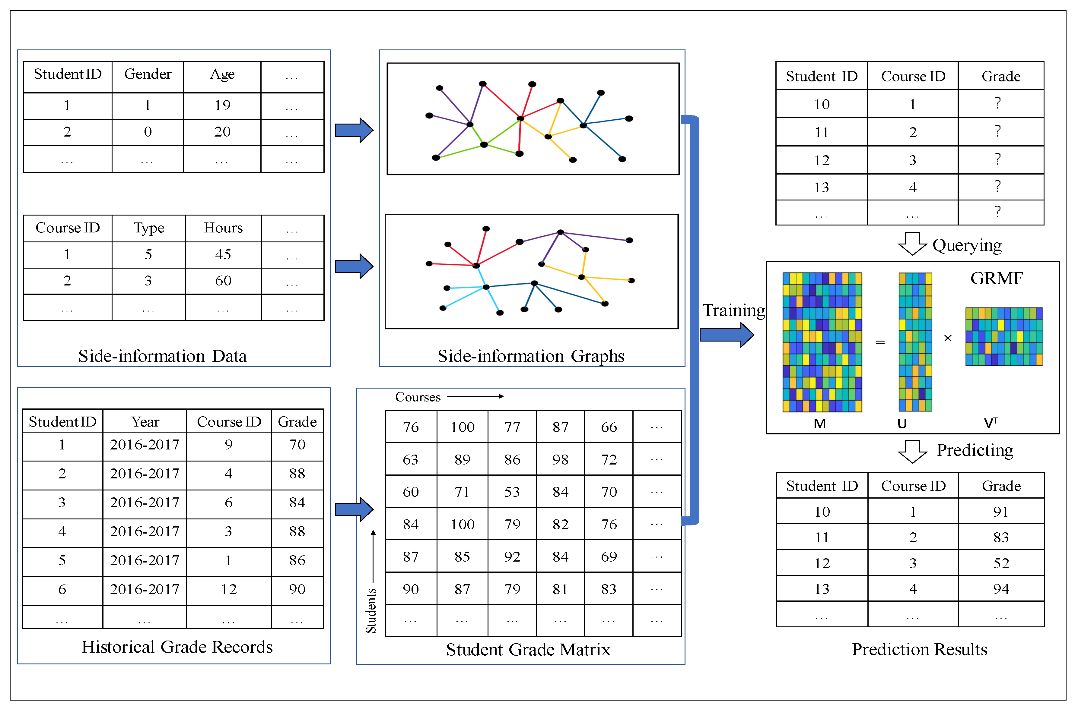
Figure 1. The proposed workflow of student grade prediction using GRMF.
Applsci 10 01755 g001
Figure 2. The value of Err1 versus iterations of Graph Regularized Robust Matrix Factorization (GRMF) on toy dataset.
Applsci 10 01755 g002
Figure 3. The effects of the parameters of GRMF on the Err1.
Applsci 10 01755 g003
Figure 4. The PNSRs of Image recovery with Gaussian noise.
Applsci 10 01755 g004
Figure 5. Evaluation of image recovery with Gaussian noise in term of PSNR. The black line that marked with “Corrupted” means the PNSR of the corrupted images.
Applsci 10 01755 g005
Figure 6. The Results of Image recovery with salt-and-pepper noise.
Applsci 10 01755 g006
Figure 7. Evaluation of image recovery with Salt-and-pepper noise.
Applsci 10 01755 g007
Figure 8. The effects of the parameters of GRMF on the Err1 and Acc.
Applsci 10 01755 g008
Table 1. Err1 and RMSE on toy dataset.
Err1RMSE
GRMF0.7350.957
MF1.5491.007
GRALS0.7701.008
RMF-MM0.7761.104
Table 2. The size of training sets and test sets.
Academic TermTraining SetTest Set
117,4253189
220,7792043
322,8212692
425,5061473
526,9492063
629,045219