Abstract
The mean age of air (MAA) is one of the most useful parameters in evaluating indoor air quality in natural ventilated buildings. Its evaluation is generally based on the CO2 monitoring within the environment; however, other methods can be found in the literature, but they have not always led to satisfactory results. In this context, the present paper is focused on two main topics: the effect of the windows airtightness and of the environmental conditions on MAA and the application of artificial neural network (ANN) for the CO2 prediction within the room. Two case studies (case study 1 located in Terni and case study 2 located in Perugia) were investigated, which differ in geometric dimensions (useful area, volume, window area) and in airtightness of windows. The indoor and outdoor environmental conditions (air temperature, pressure, relative humidity, air velocity, and indoor CO2 concentration) were monitored in 33 experimental campaigns, in four room configurations: open door-open window (OD-OW); closed door-open window (CD-OW); open door-closed window (OD-CW); closed door-closed window (CD-CW). Tracer decay methodology, according to ISO 16000-8:2007 standard, was compiled during all the experimental campaigns. A feedforward ANN, able to simulate the indoor CO2 concentration within the rooms, was then implemented; the monitored environmental conditions (air temperature, pressure, relative humidity, and air velocity), the geometric dimensions (useful area, volume, window area), and the airtightness of windows were provided as input data, while the CO2 concentration was used as target. In particular, data of 19 experimental campaigns were provided for the training process of the network, while 14 were only used for testing the reliability of ANN. The CO2 concentration predicted by ANN was then used for the MAA calculation in the four room configurations. Experimental results show that MAA of case study 2 is always higher, in all the examined configurations, due to the higher airtightness characteristics of the window and to the higher volume of the room. When the difference between indoor and outdoor temperature increases, the MAA increases too, in almost all the investigated configurations. Finally, the CO2 concentration predicted by ANN was compared with experimental data; results show a good accuracy of the network both in CO2 prediction and in the MAA calculation. The predicted CO2 concentration at the beginning of experimental campaigns (time step 0) always differs less than 2% from experimental data, while a mean percentage difference of −18.8% was found considering the maximum CO2 concentration. The MAA calculated using the predicted CO2 of ANN was greater than the one obtained from experimental data, with a difference in the 0.5–1.3 min range, depending on the configuration. According to the results, the developed ANN can be considered an alternative and valuable tool for a preliminary evaluation of MAA.
1. Introduction
The building envelope plays a fundamental role in energy balance, in fact, more and more strict limit values for the thermal performance parameters (such as thermal transmittance of transparent and opaque components) are required for the heat loss reduction. Natural and mechanical ventilation significantly influence the thermal loads and the thermal comfort; however, mechanical ventilation could be more effective than the natural one for indoor air quality [1,2,3], but it is responsible for higher energy demand. The contribution of natural ventilation is also significant, and airtight frames for glazing systems are more and more adopted, in order to reduce energy consumption [4,5,6,7,8]. Almeida et al. [9] showed that the windows’ permeability indices can have a very wide range of variability (from 4.8 to 96.4 m3/h m2), due to the year of construction, the frame material, and the opening system. Nevertheless, if the airtightness performance is too high, it can contribute to deteriorating indoor air quality (IAQ), due to the less air exchange [10]. Furthermore, the air replacement is very important, especially in natural ventilated buildings, where it is almost exclusively granted by the infiltrations and by opening the windows.
Several parameters have been proposed since the 1990s to characterize the air-flow patterns, such as local mean age of air (MAA) [11], contaminant removal effectiveness, or relative contaminant removal effectiveness [12], and air exchange efficiency [13], but the mean age of air (MAA) is widely used in evaluating the indoor air quality of buildings. The age of air is the mean time that a particle takes to travel from an inlet point (such as the outdoor air intake) to the measurement point; it can be used to calculate the air-change effectiveness of a single-zone or a multi-zone system [11] and the air distribution in buildings [14]. The amount can be measured by injecting tracer gases at the inlet and recording their concentration at the position of interest. Van Buggenhout et al. [14] in 2006 proposed a data-based mechanistic (DBM) modeling technique to assess ventilation performance in a forced ventilation type of building. Several models and algorithms were also proposed, in order to create real-time maps of chemical concentrations in air [15], but they were not always appropriate for building applications, especially in naturally ventilated ones, where the control of air exchange in the room is fuzzy and more difficult to be modeled [16]. In these cases, experimental campaigns are more suitable for evaluating indoor air quality performance of buildings, and different measurement techniques are available for air motion characterization in rooms [17]. The tracer gas technique, based on the decay method and in compliance with ISO 16000-8:2007 [18], is a simple measurement methodology that allows calculating MAA in several experimental configurations. Experimental data can be used to validate CFD (Computational Fluid Dynamics) models, able to simulate the CO2 concentration inside the room and then to calculate the MAA in different conditions. In the literature, CFD models are most focused on mechanical ventilated buildings, because the modeling is easier and the solutions are in general convergent. In natural ventilated buildings, the air movement is more difficult to follow and in many cases, the solutions of the motion fields are not convergent. Aijun et al. [19] studied the ventilation effectiveness in an aircraft cabin mockup by means of both experimental campaigns (using the volumetric particle tracking velocimetry (VPTV) technique) and CFD model simulations, while Chanteloup and Mirade [20] applied CFD simulations in forced ventilation food plants. The numerical model was also used for studying the influence of the characteristics and the placement of a complex low-velocity air diffuser on the thermal comfort and indoor air quality [21] and the characteristics of incoming air, when it is supplied via individual or multiple inlets [22]. It was furthermore applied to the air flow field investigation, MAA and CO2 distribution, and air-change efficiency when inside a bedroom the heights of the supply air outlet is varied [23], or to particular building ventilation devices such as wind towers and wind-catchers [24,25]. Different applications of similar CFD models, far from the aim of the present paper, were proposed in the chemical and biopharmaceutical fields [26,27] or in the evaluation of the MAA in the outside city ventilation [28].
In natural ventilated buildings, the experimental approach is necessary in order to evaluate the indoor air quality performance; further useful information could be also obtained by questionnaire surveys [29,30].
In a previous study [31], the authors investigated the wind-forced natural ventilation rates of an office both with an experimental and a numerical procedure, by using the CFD code Fluent, and MAA was calculated. Experimental data were used to validate the numerical method. The simulation results were in a good agreement with the experimental ones only for the lower values of the MAA, in a configuration with both door and window opened; for higher values (especially in the configurations with closed window), the numerical solution was not convergent, therefore an experimental approach is necessary. In these cases, the environmental parameters could have an important role in determining the air exchange performance of a room, such as reported in [32], where the influence of the supply air temperature on the mean local age of air was investigated considering a stratum ventilated office.
In the literature, other different approaches are also studied and applied in the engineering field, which can be useful for this kind of investigation. Artificial neural networks (ANN), are the most used in prediction problems, i.e., when an output is calculated starting from known parameters [33,34,35,36]. The authors have also studied the ANN in different kinds of applications, such as energy demand [37], thermal comfort [38], and indoor air temperature [39] prediction; in each one, the strengths and weakness of ANN were highlighted. According to these works, artificial neural networks could be a very useful tool for CO2 concentration prediction within the room, starting from a few input parameters. It is worth noting that in all the papers, a feedforward network, and in particular, a fitting neural network, was always used for predicting the energy demand, the PMV (Predicted Mean Vote) index, or the air temperature. In these studies, the same pattern of ANN was used, i.e., one input, one hidden, and one output layer. Only in [36,39], two hidden layers were needed for obtaining a good reliability of the ANN.
According to the state of the art, in the present paper, two main topics are investigated: the effect of the windows airtightness and of the environmental conditions (such as temperature and pressure) on the ventilation rate and the application of ANN for the CO2 prediction within the room.
Both topics represent a significant novelty, because they are a first tentative to:
- Establish a correlation of the mean age of air (MAA) with the environmental conditions. As far as the authors’ awareness, only a few data are available in the scientific literature about this topic;
- Simulate the CO2 concentration by using artificial neural network. No applications of ANNs in this field were found in the literature, therefore, it can lead an innovative contribution to the scientific literature.
Two offices located in two cities of the Umbria region—central Italy were chosen as case studies. They mainly differ by geometric characteristics (volume differs for about 30%) and by the airtightness class of the window (considered as Class 1–2 and Class 4, respectively). Thirty-three experimental campaigns were overall carried out in different seasons, environmental conditions, and with different room configurations.
The tracer decay measurement methodology was followed, in compliance with ISO 16000-8 [18,40], by using CO2 as tracer gas. The CO2 concentration and all the environmental conditions were monitored at established time intervals in each survey. The MAA was also calculated for all the experimental campaigns by using a numerical integration technique (the trapezoid method), and the results of the two case studies were compared and discussed with relation to the geometrical characteristics of the rooms, the airtightness characteristics of the windows, and considering its variation with the mean difference of environmental parameters.
An ANN was then implemented by using a methodology purposely developed for the intended objectives. Specifically, data of only 19 experimental campaigns were provided for the trained process, while the last 14 surveys were used for testing the generalization of the network, i.e., for checking the reliability of ANN with data different from those used for the training process [33,34,35,36,37,38,39]. The paper is structured as follows: Section 2 presents the case studies, the employed measurement methodology, the instruments characteristic, and the developed methodology for ANN implementation. Section 3 is devoted to the discussion of results related to mean age of air correlated with the environmental conditions and CO2 concentration prediction, by using artificial neural network. Finally, conclusions are drawn in Section 4.
2. Materials and Methods
2.1. Case Studies
Two offices located in two cities of the Umbria region, in central Italy (Terni and Perugia, about 80 km far from each other) were chosen as case studies. The first one, indicated as case study 1, is located at the University of Engineering in Terni, while the second one, named case study 2, is located at the Department of Engineering in Perugia. The two offices are shown in Figure 1 (case study 1) and in Figure 2 (case study 2).
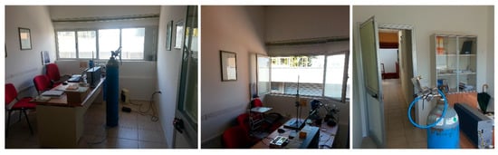
Figure 1.
Room in Terni (case study 1) during the measurement campaigns.
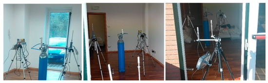
Figure 2.
Room in Perugia (case study 2) during the measurement campaigns.
The case study 1 is the same already investigated in [31] and it is located at the first floor of the building with a volume of about 32 m3 and a window surface of about 2.5 m2. However, less than 1 m2 is the opening part of the window. The characteristics of airtightness of the window can be estimated with reference to the standard EN 12207:2016 [41] as Class 1–2, corresponding to a flow rate per square meter of surface area in the 50–27 m3/hm2 range.
The case study 2 is located in Perugia, at the ground floor, with a volume of about 44 m3 and a window of about 2.2 m2 total surface; about 1.8 m2 is the opening part of the window. In this case, the airtightness of the window was estimated as Class 4 [41], corresponding to about 3 m3/hm2.
Both the offices have similar bordering conditions; only one wall border toward the outside, two sides border towards aisles, and one with another office. The main features of the investigated rooms are reported in Table 1.

Table 1.
Main features of the two investigated rooms.
2.2. Measurement Methodology
The measurement methodology, already set up in a previous work [30], is in compliance with ISO 16000-8 [18] and it is based on the decay method with the use of a single tracer gas. Among the various traces gases suggested by the standard (such as nitrogen, helium, argon, and carbon dioxide), CO2 was chosen, due to its facility to be detected and to its suitable characteristics (chemically inert, non-toxic, without risk for health in the concentration ranged used, stable, unable to be absorbed by walls and furniture) [40].
The principle of decay method is based on marking the air in the ventilated room with the tracer gas and to evaluate the time necessary to replace the marked air with unmarked air.
The tracer gas was supplied by a compressed tank of CO2, with a critical orifice and a gas flow rate measurement device (Figure 3). The minimum flow rate and the duration of the CO2 introduction were established in compliance with the standard [18] as a function of the volume of the room. In order to create a uniform gas concentration in the investigated volume, fans were switched on before each test; this procedure allowed to obtain a uniform concentration of the gas tracer in different points of the room volume, such as verified in the previous work [31]. The presence of people in the test room is a carbon dioxide source, so its concentration was recorded before the tracer gas introduction, in order to have a reference value for the MAA calculation; operators stayed outside the room during the measurements, but the limits of the European Agency for Safety and Health at Work (2010) were anyway considered. As the maximum concentration was reached, the decay started. The acquisition rate of the concentration of the gas tracer was generally 1 min; longer acquisition rates (2, 3, 5, and 10 min) were set when the decay was very long-lasting, especially in the configurations with the closed window. The CO2 concentration was registered for a total time greater than the expected average age of air.
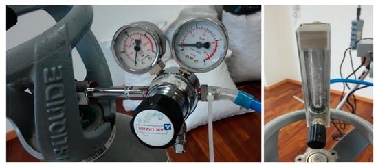
Figure 3.
Tracer gas supplier: pressure adaptor (left) and flow meter (right).
We clarified this point. All the instrumentations were placed in a central position of the room, when possible, and in particular:
- A CO2 pressurized tank was placed in a central position of the room;
- The instrumentation for recording CO2 concentration was placed at about 1.2 m of height;
- The instrumentations for recording the indoor environmental conditions were placed next to the CO2 pressurized tank and at 1.2–1.5 m of height;
- The outdoor conditions were monitored by placing the instrumentations outdoor next to the window of the investigated room.
After recording the gas concentration in a representative point during the decay time, the local mean age of air is obtained as follows [16], by solving the integral in the numerator by means of the trapezoid method:
where:
- MAA is the mean age of air;
- φ is the tracer gas concentration;
- ∆t is the time acquisition rate;
- t0 is the initial time;
- te is the time when an exponential decay has been ascertained (linear logarithmic plot);
- λtail is the absolute value of the slope from a plot of the logarithm of concentration as a function of time in the last exponential part of the decay.
In both the case studies and when possible, the following four room configurations were also investigated:
- OD_OW: open door-open window;
- CD_OW: closed door-open window;
- OD_CW: open door-closed window;
- CD_CW: closed door-closed window.
The configurations and the monitored period of each experimental campaign are reported in Table 2. The sequential number shown in Table 2 was set by considering the following criteria: firstly, the four configurations of case study 1 (OD_OW, CD_OW, OD_CW, and CD_CW) and then the ones related to case study 2 were considered.
Table 2.
Main features of the two investigated rooms.
2.3. Instruments
The CO2 was supplied by means of a pressurized tank, equipped with a pressure adaptor (DIM 200-15-25.S) in stainless steel 316 L and Hastelloy C (Figure 3 left) and a flux meter Kobot Instrument Kit KDG-212-JNG600 for very low flow rates, with a spherical suspension floating probe (Figure 3 right).
Two different instrumentations were used for measuring and recording the CO2 concentration in the two case studies: a micro-GC VARIAN Inc CP-4900 model, with a thermal conductivity detector (TCD) (case study 1), and an infrared CO2 concentration probe (BSO103) equipped with an aspiration pump and connected to a multi-acquisition system LSI BABUC (case study 1). The GC system is available at the Terni site of the university (case study 1) and it is difficult to be transported, while the BABUC system is very manageable and easy to be transported. Therefore, it was not possible to use the GC system in the Perugia office (case study 2). Before starting the measurements in Perugia, some spot CO2 concentrations were contemporary measured at the Terni site (case study 1) with both the instrumentations. Results show a good agreement between data recorded by the two different systems, therefore the BABUC system, simpler than the GC one, was used for case study 2.
The indoor conditions were monitored by means of a multi-acquisition system LSI BABUC, while the outdoor conditions were monitored by means of a multi-acquisition system DeltaOHM, both equipped with several probes. Temperature and relative humidity, both inside and outside, were also monitored in other points by means of Tiny Tag probes.
The characteristics of the instruments and of the probes are reported in Table 3.
Table 3.
Experimental facility and accuracy of equipment.
2.4. ANN Implementation
The literature analysis highlighted the peculiarity and the weakness of the available methodology for the MAA calculation; as reported, the most common method consists in the use of the CFD code which allows to simulate the motion field within a room considering several and different boundary conditions. However, as highlighted in [31], the main critical issues of CFD simulation is the lack of convergence of solution, which makes the result unreliable.
The convergence of solution is influenced by many parameters, such as the mesh size, time step, the equation models, and so on, which can lead to high computational resources requirement and high time consuming. For these reasons, in this paper, an alternative method for the CO2 simulation and MAA calculation was tried; in particular, according to the literature analysis, the first application of the ANN for the CO2 prediction was attempted.
Neural networks are mathematical models able to simulate the learning process of the biological neural system and can be trained based on experimental data, so they are not programmed [42]. For the implementation of a network able to predict the CO2 concentration within the room, a similar methodology developed in previous works [37,38,39] was adopted. A multi-layer perceptron (MLP) network with only one hidden layer was trained by using Leverberg–Marquardt backpropagation algorithm and by providing several inputs and one target for the training process: the CO2 concentration was chosen as the target parameter and the following parameters were supplied as inputs:
- Room configuration (OD_OW, OD_CW, CD_OW, CD_CW);
- Acquisition time (t);
- Difference between indoor and outdoor air temperature (∆T);
- Difference between indoor and outdoor air velocity (∆v);
- Difference between indoor and outdoor air relative humidity (∆RH);
- Difference between indoor and outdoor air pressure (∆P);
- Usable floor area of the case studies (Afloor);
- Net volume of the case studies (Vnet);
- Opening area of the environment (window and door);
- Perimeter of the opening surfaces (window and door);
- Airtightness class of the window (Class);
- CO2 gas injection step by step (CO2supply).
It is worth noting that time and CO2 gas injection are two key parameters to be supplied, being the only ones closely related to the increase of CO2 within the room, but all the considered parameters affect its decay over time. Furthermore, for the ANN implementation, the CO2 gas injection was set to the established values only for the time steps the tank was open, and set to zero for all the other time steps. As in [37,38,39], a sensitivity analysis was performed in order to establish the best number of neurons to be used in the hidden layer and to minimize the error of the network. The procedure adopted for the implementation of the artificial neural network able to predict the CO2 concentration within the room is shown in Figure 4. In particular, the experimental campaigns used for the training and testing processes are highlighted; they were chosen randomly; the only criterion adopted was to choose for both processes at least one survey for each configuration and case study. It is important to point out that in Figure 4 the algorithm developed after the training process was named ANNCO2concentration; i.e., it is the name of the trained network which can be used for CO2 prediction. The accuracy of the training process is checked by considering two control parameters: regression value (R) and the mean square error (MSE). The first one allows to correlate the outputs of ANN with experimental values (target) and when it is equal to 1, it means that a perfect correlation is found. MSE allows to evaluate the most probable error returned by the network, therefore the more the MSE is close to 0, the more the accuracy of ANN is high.
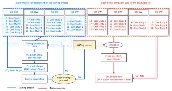
Figure 4.
Implementation procedure adopted for the development of artificial neural network able to simulate the CO2 concentration within the rooms.
3. Results and Discussion
3.1. MAA Correlation with the Environmental Conditions
According to Equation (1) [18], the MAA depends on the CO2 decay step by step within the environment, so it also depends on the environmental conditions. Firstly, the correlation between CO2 concentration and environmental condition and then the one with MAA will be discussed. For the clarity of discussion, the mean values calculated for each experimental campaign divided for case studies and experimental configurations are reported in Table 4.
Table 4.
Environmental parameters measured during the experimental campaigns for each investigated configuration (OD_OW, CD_OW, OD_CW, and CD_CW).
Figure 5 shows the CO2 concentration within the room as a function of the difference of the main environmental conditions (temperature, pressure, air velocity, and relative humidity). The CO2 concentration monitored step by step within the room does not seem to be significantly affected by the environmental conditions (white dots with black edges); however, the maximum values reached in each experimental campaign (red dots) seem to be. In fact, the higher maximum values of CO2 were found in the following range: ∆T in 7–9 °C, ∆P in −3–3 hPa, ∆v in −0.27–0 m/s, and ∆RH in −34%–−10%.
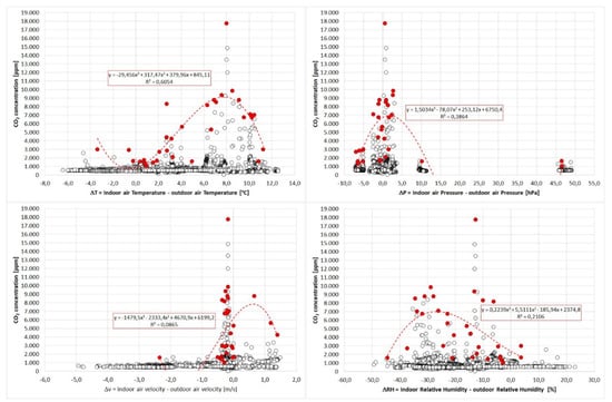
Figure 5.
Correlation between CO2 concentration and environmental conditions.
This analysis was studied in depth by considering the different configurations and each specific case study. In particular, Figure 6 shows the maximum values of CO2 for the four room configurations and for the two investigated case studies (case study 1 in white and black edges, case study 2 in red). As expected, the maximum value of concentration also depends on the room configuration, and it varies significantly for the two investigated case studies. The highest values of CO2 were reached in the case study 1, which also seems to be more affected by the environmental conditions, contrary to the one monitored in the case study. CO2 values monitored in case study 2 are in fact very close to each other, so they do not seem to be significantly affected by both environmental conditions and room configurations.
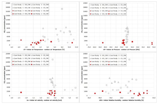
Figure 6.
Correlation between CO2 concentration and environmental conditions divided for case studies and experimental campaign configuration.
Based on these results, the MAA indicator was calculated for each experimental campaign. Figure 7 shows all the MAA values and the average ones calculated for each configuration and case study. As highlighted, the MAA increases exponentially varying the room configuration; in particular, for both case studies the highest values were calculated for the last configuration (CD_CW), which can be considered the worst room configuration. The average values calculated for OD_OW, CD_OW, and OD_CW are very close for the two case studies and equal to 4.7–5.3 min, 17.2–22.1 min, and 31.1–33.1 min for Terni (1) and Perugia (2), respectively. Only for the CD_CW configuration, a higher difference of the MAA mean value was focused (163 min vs. 143.6 min); according to the results, in all the configurations, a higher MAA value was found for the case study 2, probably due to both the higher window airtightness and bigger volume of the room.
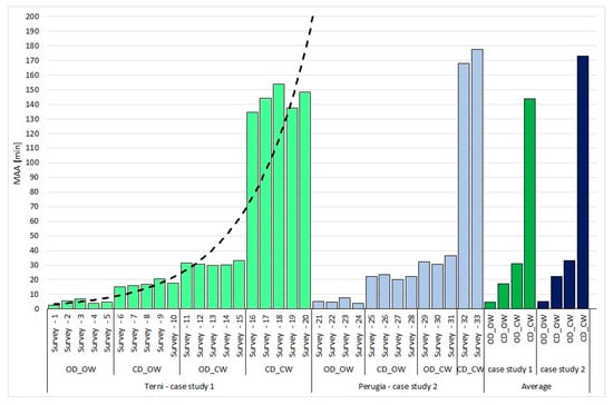
Figure 7.
MAA (Mean Age of the Air) calculated for each experimental campaign and configuration, and MAA average values obtained for the two case studies.
Once the MAA was calculated, the correlation with environmental conditions was investigated. Firstly, the correlation of MAA with environmental parameters was investigated considering each case study and each room configuration. Results are shown in Figure 8 and Figure 9. In these figures, the following criteria and legend were adopted:
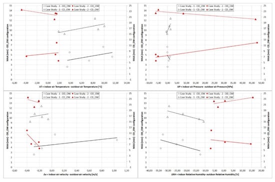
Figure 8.
Correlation between MAA and environmental conditions—OD_OW and CD_OW configurations.
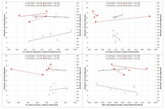
Figure 9.
Correlation between MAA and environmental conditions—CD_OW and CD_CW configurations.
- Case study 1 is always drawn with white indicators and black edges, while case study 2 is drawn in red;
Interesting correlations can be found when considering the mean difference of all the environmental parameters. MAA increases when the difference between the indoor and outdoor mean temperature increases, in all the studied configurations, except for OD_OW (case study 2) and OD_CW (case study 1): the dependence is emphasized for the configurations with the closed window, where a higher slope of the regression lines is found. A specular trend was instead found considering the mean difference of relative humidity. Furthermore, considering the mean difference of air velocity and of air pressure, an opposite trend for the two case studies was also highlighted; in fact, when MAA indicator increases for one case study, it decreases for the other one. For instance, considering the difference of the air pressure, for case study 1, the MAA increases in CD_OW and OD_CW configurations and decreases in OD_OW and CD_CW ones; the same indicator decreases in CD_OW and OD_CW and increases in OD_OW and CD_CW for the case study 2. The same trend can be highlighted considering the difference of the air velocity. This important divergence can be due to the different characteristics of environments (volume), to the dimensions of the openings (opening surfaces), and to the window airtightness class.
In order to study the results of the two different case studies in depth, MAA was also compared with the air change (G), calculated as shown in Equation (2) considering the monitored environmental conditions, the total opening area (window and door of rooms when they are open), and the room volume. All the data is reported in Table 1.
where:
- v is the monitored indoor or outdoor air velocity (m/h);
- OA is the opening surface (window and door when they are open) of the room (m2);
- ρ is the permeability class of the window, according to [41] (m3/hm);
- L is the perimeter of the considered opening surface (m);
- V is the volume of the room (m3).
According to Equation (2), G represents the air volume changed in one hour within the room. In Figure 10, it is possible to notice a significant difference in behavior of the regression lines drawn for the two case studies. The slope of the lines (case study 1 in black and case study 2 in the red) mainly depends on the airtightness of the windows; in fact, G tends to increase with decreasing of the window airtightness class (Class 1–2 for the case study 1), due to the higher air permeability. In particular, as expected, it is worth noting that the opening surfaces influence the MAA indicator especially in a room with windows with higher airtightness class; it means that in the case study 2, the opening surface area is more effective than case study 1, despite the difference of total opening area of just 1 m2.
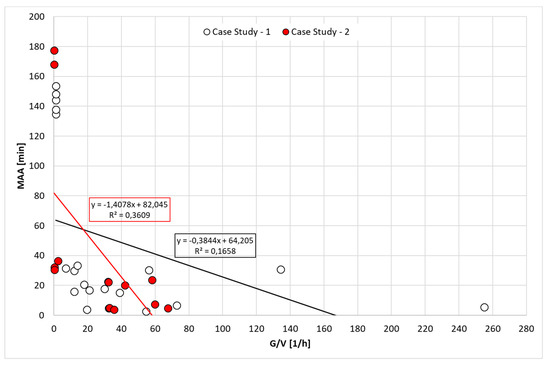
Figure 10.
Correlation between MAA with opening area and volume.
3.2. Artificial Neural Network for CO2 Concentration Prediction
According to Section 2.4 and to the adopted implementation procedure (Figure 4), several ANNs were trained by varying the number of neurons to be used in the hidden layers. For the sake of brevity, only the results of the best trained ANN will be reported. The best ANN was obtained by using 173 neurons in the hidden layer which has the highest regression value (equal to 0.967 for all the training processes) and the smallest MSE (the most probably error is in −50–50 ppm range). The trained ANN was then tested for the CO2 prediction with the other experimental campaigns, as shown in Figure 4.
Results related to the implementation of the network are shown in Figure 11 and Figure 12. In particular, Figure 11 shows the comparison between the CO2 values monitored during the experimental campaigns (on the abscissa—target) and the one simulated by ANN (on the ordinate—ANN output) for both the considered processes (training in black dots and testing in red box). In this figure, in order to highlight the accuracy of the ANN, the regression line for each process was also drawn: R2 values equal to 0.98 and 0.99 were found for the training and testing processes, respectively.
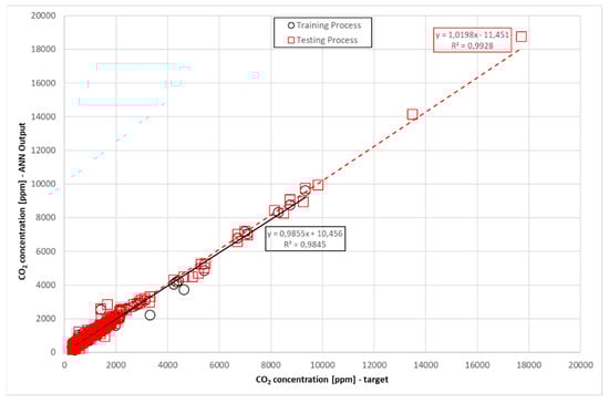
Figure 11.
CO2 prediction comparison: experimental data vs. ANN (Artificial Neural Network) outputs (training process in black and testing one in red).
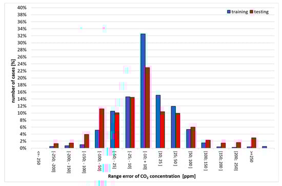
Figure 12.
MSE (Mean Square Error) of ANN (Artificial Neural Network): range of error returned by ANN in the training and testing processes.
Figure 12 allows to confirm the reliability of the trained ANN; the MSE in the two processes (training in blue bars and testing in red ones) is reported. Particularly, it shows that the most probably error returned by the ANN is in the −50/50 ppm range (84.7% of cases) for the training process, and −100–100 ppm range (84% of cases) for the testing one.
According to the results, the trained ANN can be considered reliable; so, the simulated CO2 concentration can be used for the MAA calculation. In Table 5 the comparison of the starting concentration (C0—the one monitored or simulated at the time step equal to 0), the maximum CO2 concentration reached during each survey (Cmax), and MAA calculated by using ANN output and experimental one are shown. Besides, surveys in red in Table 5 are related to the experimental campaigns used for the testing process, the other ones for the training.
Table 5.
C0, Cmax, and MAA comparison: experimental data vs. ANN outputs (surveys on rows in red were used for the testing process, the other ones for the training).
It is worth noting that the CO2 concentration simulated by ANN at time step 0 is always close to the real values; i.e., the different between the two values is always lower than 10 ppm (always lower than 2%). It means that the ANN allows to correctly simulate the real concentration within the room, starting from the environmental conditions. The maximum concentration simulated by ANN, on the other hand, presents much higher error, with peaks of −140%. This means that the network is not always able to correctly predict the maximum values of CO2 reached within the environment. In fact, only in about 50% of surveys an error lower than ± 30% was found. However, despite the different maximum value of CO2 concentration simulated by ANN, the MAA calculated starting from ANN data is very close to the experimental one except for a very few cases (mainly in OD_OW configuration). In this case, the mean error is about 1–2 min.
As shown in Table 5, the higher relative error was found in OD_OW configuration, which is the one with the lowest values of MAA; in fact, as also reported in Table 6, the mean values of MAA derived from ANN data differ for a maximum of 2–3 min for OD_OW. Furthermore, the higher errors were found in only specific experimental campaigns; in particular, considering the ones used for the training process, the relative error is always lower than 6% except for OD_OW configuration (equal to 45% and 17.5%), but in this case the absolute error is about 1–2 min, therefore it can be considered acceptable.
Table 6.
MAA mean values comparison: experimental data vs. ANN outputs.
Considering the experimental campaign used for the testing process, the relative error has slightly increased in all the room configurations: about 66% and 24% for OD_OW, and lower than 10% in all the other configurations, except for CD_OW of case study 1 (13.7%). However, also in this case, the absolute error related to OD_OW configuration is about 2–3 min, so it can be considered acceptable too.
Furthermore, all the results shown in Table 6 are in agreement with the trained ANN; in fact, as also shown in Figure 12, the network tends to predict a CO2 concentration with a slightly higher error in the testing process (most probably error in −100 + 100 ppm), so it can lead to less accuracy in the MAA calculation.
4. Conclusions
Indoor air quality in natural ventilating buildings is strictly dependent on windows frame airtightness. The more and more pressing norms aiming at energy saving in buildings played an important role in making airtightness in buildings more effective: it contributes to energy saving but, on the other hand, it can also cause indoor air quality deterioration.
In this context, in the present paper, two case studies were investigated: two natural ventilated rooms with different airtightness class of the window frame. The first one, with a volume of about 32 m3, is characterized by a window with airtightness Class 1/2 (corresponding to 50–27 m3/hm2 of air of infiltration). The airtightness class of the second one, with a volume of about 44 m3, is 4 (3 m3/hm2 of air of infiltration).
The mean age of air (MAA) was experimentally evaluated in compliance with ISO 16000-8:2007 [16], in thirty-three different experimental campaigns, twenty for case study 1 (situated in Terni) and thirteen for case study 2 (situated in Perugia). During each experimental campaign, four different room configurations were investigated: open door-open window (OD_OW), closed door-open window (CD_OW), open door-closed window (OD_CW), and closed door-closed window (CD_CW). During the experimental campaigns, the main indoor and outdoor environmental parameters were also monitored.
The CO2 concentration and the MAA values obtained for the two case studies were then correlated. Results show that:
- MAA values increase from the configuration OD_OW to the configuration CD_CW, with an exponential trend and with a very significant gap between the configurations with open and closed window, while the configuration of the door has a less influence;
- MAA calculated for case study 2 is substantially higher with respect to the ones related to case study 1. The difference found in the configurations with closed window is mainly due to the airtightness of the frame, while the one in the configurations with open window is probably due to the volume of the room;
- A similar behaviour is observed when comparing the MAA with air flow rate per room volume (G/V), where G represents the air change and V the volume of the room;
- The difference between the two case studies is more emphasises when considering only the G values, confirming that the opening surfaces have more influence on MAA indicator in a room with windows with the higher airtightness class;
- MAA increases when the difference between the indoor and outdoor mean temperature increases, in almost all the studied configurations, with a more emphasized dependence for the configurations with the closed window;
- An opposite trend for the two case studies was observed when comparing the MAA with the difference of air pressure and air velocity;
- An influence on MAA indicator specular with respect to the one of the temperature was observed for air relative humidity difference;
- A more emphasized dependence is found for the configurations with the closed window.
Finally, an artificial neural network (ANN) was implemented, able to predict the CO2 concentration within the room; 12 parameters related to geometric dimension of the room, permeability characteristics of windows, and environmental conditions were provided as input data, while the CO2 concentration was used as target. A multi-layer perceptron (MLP) neural network was trained by using data of 19 experimental campaigns, while the last 14 ones were used for testing and checking the reliability of generalization of the network. Results show a good agreement between experimental CO2 concentration and the one predicted by the ANN in all the experimental campaigns; in particular, the starting concentration (at time step 0) simulated by the ANN is always very close to the real one (mean error lower than 1%). A higher mean error was found for the maximum CO2 concentration reached in about 50% of the surveys. However, it does not involve a wrong evaluation of the MAA indicator; according to the results, the MAA calculated starting from CO2 predicted by ANN differs from the experimental one of about a few minutes (2–3 min for OD_OW, and maximum 10 min for CD_CW). Therefore, the ability to use ANN for the evaluation of MAA has been demonstrated.
It can be also concluded that both window frame airtightness and environmental conditions, especially indoor and outdoor air temperatures, play an important role in air replacement in natural ventilated buildings and in indoor air quality. Therefore, it has to be carefully taken into account when solutions aiming at reducing air infiltration for energy savings are adopted.
Author Contributions
Conceptualization, C.B.; methodology, C.B. and D.P.; investigation, D.P.; writing—original draft preparation, C.B. and D.P.; writing—review and editing, C.B.; supervision, C.B. All authors have read and agreed to the published version of the manuscript.
Funding
This research received no external funding.
Acknowledgments
The Authors wish to thank Maurizio Tomassoli for his precious contribution during the measurement campaigns in Perugia.
Conflicts of Interest
The authors declare no conflict of interest.
References
- Lei, Z.; Junjie, L.; Jianlin, R. Impact of various ventilation modes on IAQ and energy consumption in Chinese dwellings: First long-term monitoring study in Tianjin, Tunisia. Build. Environ. 2018, 143, 99–106. [Google Scholar] [CrossRef]
- Anand, P.; Cheong, D.; Sekhar, C. Computation of zone-level ventilation requirement based on actual occupancy, plug, and lighting load information. Indoor Built Environ. Sage J. 2019. [Google Scholar] [CrossRef]
- Anand, P.; Sekhar, C.; Cheong, D.; Santamouris, M.; Kondepudi, S. Occupancy-based zone-level VAV system control implications on thermal comfort, ventilation, indoor air quality and building energy efficiency. Energy Build. 2019, 2014, 109473. [Google Scholar] [CrossRef]
- Omrani, S.; Garcia-Hansen, V.; Capra, B.R.; Drogemuller, R. On the effect of provision of balconies on natural ventilation and thermal comfort in high-rise residential buildings. Build. Environ. 2017, 123, 504–516. [Google Scholar] [CrossRef]
- van den Bossche, N.; Janssens, A. Airtightness and watertightness of window frames: Comparison of performance and requirements. Build. Environ. 2016, 110, 129–139. [Google Scholar] [CrossRef]
- Fernández-Agüeraa, J.; Domínguez-Amarillo, S.; Sendra, J.J.; Suárez, R. An approach to modelling envelope airtightness in multi-family social housing in Mediterranean Europe based on the situation in Spain. Energy Build. 2016, 128, 236–253. [Google Scholar] [CrossRef]
- Gillott, M.C.; Loveday, D.L.; White, J.; Wood, C.J.; Chmutina, K.; Vadodaria, K. Improving the airtightness in an existing UK dwelling: The challenges, the measures and their effectiveness. Build. Environ. 2016, 95, 227–239. [Google Scholar] [CrossRef]
- Cuce, E. Role of airtightness in energy loss from windows, Experimental results from in-situ tests. Energ. Build. 2017, 139, 449–455. [Google Scholar] [CrossRef]
- Almeidaa, R.M.S.F.; Ramos, N.M.M.; Pereira, P.F. A contribution for the quantification of the influence of windows on the airtightness of Southern European buildings. Energy Build. 2017, 139, 174–185. [Google Scholar] [CrossRef]
- Ramos, N.M.M.; Almeida, R.M.S.F.; Curado, A.; Pereira, P.F.; Manuel, S.; Maia, J. Airtightness and ventilation in a mild climate country rehabilitated social housing buildings—What users want and what they get. Build. Environ. 2015, 92, 97–110. [Google Scholar] [CrossRef]
- Federspiel, C.C. Air-Change Effectiveness, Theory and Calculation Methods. Indoor Air 1999, 9, 47–56. [Google Scholar] [CrossRef] [PubMed]
- Haghighat, F.; Fazio, P.; Rao, J. A procedure for measurement of ventilation ef- fectiveness in residential buildings. Build. Environ. 1990, 25, 163–172. [Google Scholar] [CrossRef]
- Etheridge, M.D. Sandberg, Building Ventilation—Theory and Measurement; John Wiley & Sons: Chichester, UK, 1996. [Google Scholar]
- van Buggenhout, S.; Desta, T.Z.; van Brecha, A.; Vranken, E.; Quanten, S.; van Malcot, W.; Berckmans, D. Data-based mechanistic modelling approach to determine the age of air in a ventilated space. Build. Environ. 2006, 41, 557–567. [Google Scholar] [CrossRef]
- Samanta, A.; Todd, L.A. Mapping chemicals in air using an environmental CAT scanning system: Evaluation of algorithms. Atmos. Environ. 2000, 34, 699–709. [Google Scholar] [CrossRef]
- Debnath, R.; Bardhan, R.; Banerjee, R. Investigating the age of air in rural Indian kitchens for sustainable built-environment design. J. Build. Eng. 2016, 7, 320–333. [Google Scholar] [CrossRef]
- Sun, Y.; Zhang, Y. An Overview of Room Air Motion Measurement: Technology and Application. HVAC R Res. 2007, 13, 929–950. [Google Scholar] [CrossRef]
- ISO 16000-8:2007. Indoor air—Part 8: Determination of Local Mean Ages of Air in Buildings for Characterizing Ventilation Conditions; International Organization for Standardization: Geneva, Switzerland, 2007. [Google Scholar]
- Wang, A.; Zhang, Y.; Sun, Y.; Wang, X. Experimental study of ventilation effectiveness and air velocity distribution in an aircraft cabin mockup. Build. Environ. 2008, 43, 337–343. [Google Scholar] [CrossRef]
- Chanteloup, V.; Mirade, P.S. Computational fluid dynamics (CFD) modelling of local mean age of air distribution in forced-ventilation food plants. J. Food Eng. 2009, 90, 90–103. [Google Scholar] [CrossRef]
- Cehlin, M.; Moshfegh, B. Numerical modelling of a complex diffuser in a room with displacement ventilation. Build. Environ. 2010, 45, 2240–2252. [Google Scholar] [CrossRef]
- Han, H.; Shin, C.; Lee, I.; Kwon, K. Tracer gas experiment for local mean ages of air from individual supply inlets in a space with multiple inlets. Build. Environ. 2011, 46, 2462–2471. [Google Scholar] [CrossRef]
- Ning, M.; Mengjie, S.; Mingyin, C.; Shiming, P.D.D. Computational fluid dynamics (CFD) modelling of air flow field, mean age of air and CO2 distributions inside a bedroom with different heights of conditioned air supply outlet. Appl. Energy 2016, 164, 906–915. [Google Scholar] [CrossRef]
- Calautit, J.K.; Hughes, B.R. Measurement and prediction of the indoor air flow in a room ventilated with a commercial wind tower. Energy Build. 2014, 84, 367–377. [Google Scholar] [CrossRef]
- Jomehzadeh, F.; Nejat, P.; Calautit, J.K.; Badruddin, M.; Yusof, M.; Zakid, S.A.; Hughes, B.R.; Yazi, M.N.A.W.M. A review on windcatcher for passive cooling and natural ventilation in buildings, Part 1: Indoor air quality and thermal comfort assessment. Renew. Sust. Energy Rev. 2017, 70, 736–756. [Google Scholar] [CrossRef]
- Russ, D.C.; Berson, R.E. Mean age theory in multiphase systems. Chem. Eng. Sci. 2016, 141, 1–7. [Google Scholar] [CrossRef]
- Bai, G.; Bee, J.S.; Biddlecombe, J.G.; Chen, Q.; Leach, W.T. Computational fluid dynamics (CFD) insights into agitation stress methods in biopharmaceutical development. Int. J. Pharm. 2012, 423, 264–280. [Google Scholar] [CrossRef]
- Hang, J.; Sandberg, M.; Li, Y. Age of air and air exchange efficiency in idealized city models. Build. Environ. 2009, 44, 1714–1723. [Google Scholar] [CrossRef]
- Huizenga, C.; Abbaszadeh, S.; Zagreus, L.; Arens, E. Air Quality and Thermal Comfort in Office Buildings: Results of a Large Indoor Environmental Quality Survey. Proc. Healthy Build. 2006, 3, 393–397. [Google Scholar]
- Leccese, F.; Salvadori, G.; Rocca, M.; Buratti, C.; Belloni, E. A method to assess lighting quality in educational rooms using analytic hierarchy process. Build. Environ. 2020, 168, 106501. [Google Scholar] [CrossRef]
- Buratti, C.; Mariani, R.; Moretti, E. Mean age of air in a naturally ventilated office: Experimental data and simulations. Energy Build. 2011, 43, 2021–2027. [Google Scholar] [CrossRef]
- Tian, L.; Lin, Z.; Liu, J.; Yao, T.; Wang, Q. The impact of temperature on mean local air age and thermal comfort in a stratum ventilated office. Build. Envion. 2011, 46, 501–510. [Google Scholar] [CrossRef]
- Gayle, C. Artificial Neural Networks New Research, Series: Computer Science, Technology and Applications; NOVA Publishers: New York, NY, USA, 2017. [Google Scholar]
- Tanaya, C.; Yeng, C.; Hua, L.; Lihua, X. A feedforward neural network based indoor-climate control framework for thermal comfort and energy saving in buildings. Appl. Energy 2019, 248, 44–53. [Google Scholar]
- Escandón, R.; Ascione, F.; Bianco, N.; Mauro, G.M.; Suárez, R.; Sendra, J.J. Thermal comfort prediction in a building category: Artificial neural network generation from calibrated models for a social housing stock in southern Europe. Appl. Therm. Eng. 2019, 250, 492–505. [Google Scholar] [CrossRef]
- Anand, P.; Cheong, D.; Sekhar, C.; Santamouris, M.; Kondepudi, S. Energy-saving estimation for plug and lighting load using occupancy analysis. Renew. Energy 2019, 143, 1143–1161. [Google Scholar] [CrossRef]
- Buratti, C.; Barbanera, M.; Palladino, D. An original tool for checking energy performance and certification of buildings by means of Artificial Neural Networks. Appl. Energy 2014, 120, 125–132. [Google Scholar] [CrossRef]
- Buratti, C.; Vergoni, M.; Palladino, D. Thermal Comfort Evaluation Within Non-residential Environments: Development of Artificial Neural Network by Using the Adaptive Approach Data. Energy Procedia 2015, 78, 2875–2880. [Google Scholar] [CrossRef]
- Buratti, C.; Lascaro, E.; Palladino, D.; Vergoni, M. Building behavior simulation by means of Artificial Neural Network in summer conditions. Sustainability 2014, 6, 5339–5353. [Google Scholar] [CrossRef]
- Gough, H.L.; Luo, Z.; Halios, C.H.; King, M.-F.; Noakes, C.J.; Grimmond, C.S.B.; Barlow, J.F.; Hoxey, R.; Quinn, A.D. Field measurement of natural ventilation rate in an idealised full-scale building located in a straggered urban array: Comparison between tracer gas and pressure-based methods. Build. Environ. 2018, 137, 246–256. [Google Scholar] [CrossRef]
- EN 12207:2017 Windows and Doors; Permeability Classification; Polish Committee for Standardization: Warszawa, Poland, 2017.
- Demuth, H.B.; Beale, M.H.; Hagan, T.M. Neural Network Toolbox: User’s Guide; MathWorks, Inc.: Natick, MA, USA, 2013. [Google Scholar]
© 2020 by the authors. Licensee MDPI, Basel, Switzerland. This article is an open access article distributed under the terms and conditions of the Creative Commons Attribution (CC BY) license (http://creativecommons.org/licenses/by/4.0/).