CRANK: A Hybrid Model for User and Content Sentiment Classification Using Social Context and Community Detection

Abstract

Recent works have shown that sentiment analysis on social media can be improved by fusing text with social context information. Social context is information such as relationships between users and interactions of users with content. Although existing works have already exploited the networked structure of social context by using graphical models or techniques such as label propagation, more advanced techniques from social network analysis remain unexplored. Our hypothesis is that these techniques can help reveal underlying features that could help with the analysis. In this work, we present a sentiment classification model (CRANK) that leverages community partitions to improve both user and content classification. We evaluated this model on existing datasets and compared it to other approaches.

1. Introduction

The state-of-the-art in the field of sentiment analysis has improved considerably in recent years, partly due to the advent of social media. Social media text imposes several limitations that are hard to overcome even for human annotators, such as the extensive use of annotations, jargon, and heavy reliance on context. Moreover, understanding a piece of content often requires following a conversation (i.e., a thread of replies) or the style and stance of the author of the content.

To solve these limitations, new approaches are starting to combine text with additional information from the social network, such as links between users and previous posts by each user. The blend of all this information can be referred to as social context. A recent work [1] analyzed the use of social context in the sentiment analysis literature, and it showed that context-based approaches performed better than traditional analysis without social context (i.e., contextless approaches). It also provided a taxonomy of approaches based on the types of features included in the context: $contextless$ approaches do not use social context at all; $micro$ approaches only use features from the users and their content; $meso$ approaches include features from other users and content, as well as connections between different users and content; and $macro$ approaches also exploit other sources such as knowledge graphs. $meso$ approaches are further divided into three categories: $mes{o}_r$ only uses relations (e.g., follower-followee); $mes{o}_i$ adds interactions (e.g., replies and likes); and $mes{o}_e$ uses Social Network Analysis (SNA) techniques to process other elements of the context and generate additional features. Comparing the performance of existing approaches seems to show that more elaborate features provide an advantage over simpler features. Simpler features are those directly extracted from the network, such as follower-followee relations ($mes{o}_r$). More complex features can be obtained from applying further processing, typically through filtering and aggregating information from the network ($mes{o}_i$), or through SNA techniques such as calculating user centrality or unsupervised community detection ($mes{o}_e$). Unfortunately, these features remain mostly unexplored and show higher variability.

This work is motivated by the following hypotheses about the use of social context:

Hypothesis 1.

$meso$ features improve user classification in the absence of $micro$ features.

Hypothesis 2.

$micro$ features improve content classification over pure $contextless$ features.

Hypothesis 3.

$meso$ features improve content classification in the absence of $micro$ features.

Hypothesis 4.

$mes{o}_e$, and community detection in particular, can improve classification compared to only using $mes{o}_i$ and $mes{o}_r$ features.

As a result, we propose a model to classify both users and content using social context. In our evaluation, we will test whether our proposal supports these hypotheses.

The social context used in our model consists of a set of users and content for a topic, as well an authorship relation between content and users, and a form of interaction or relation between users. Moreover, some of the users and content have known sentiment labels. Through community detection, we generate a network of users that belong to the same community. This network is then used to estimate the sentiment of the missing labels for users and content, i.e., it performs both user-level and content-level classification.

The estimation is based on maximizing a metric that is inspired by sentiment consistency and homophily theories. Sentiment consistency implies that the sentiment of a user on a given topic is stable over time. The homophily theory dictates that similar users are more likely to form connections. In our case, two users are similar if they share the same sentiment on a given topic.

The classification model is based on an earlier model by Pozzi et al. [2], which our model improves in two significant ways: (1) it can be used for content-level classification, and (2) in addition to using the raw relations from the social network, it can also use community detection to find weak relations between users.

The rest of the paper is structured as follows: Section 2 covers related works and concepts; Section 3 describes the classification model; Section 4 is dedicated to a description of the datasets used for evaluation and how they have been enriched with social context; Section 5 presents the evaluation of the model; Section 6 closes with our conclusions and future lines of work.

2. Related Work

This section summarizes the state-of-the-art in the fields of sentiment analysis and Social Network Analysis (SNA). It also provides a summary of the definitions and nomenclature on social context.

2.1. Sentiment Analysis

Sentiment analysis, or the process of assessing attitudes expressed in text, is hardly a new field, but its popularity has grown due to the increasing availability and popularity of opinion-rich resources such as online review sites and personal blogs [3].

The approaches in this field can be grouped into three main categories: lexicon-based, machine learning-based, and hybrid [4]. In this section, we will focus on lexicon and machine learning-based approaches, as hybrid approaches use a combination of both.

Lexicon-based approaches are potentially the simplest. They estimate the sentiment of a text using a lexicon, or associations of lexical entries (e.g., words) in a domain with one or more sentiments. Machine learning approaches apply a predictor on a set of features that represent the input. The predictors used for sentiment analysis are not very different from those used in other areas. The complexity lies in extracting useful features from the text, curating them, and applying them with the appropriate predictor [5].

Lexicon-based approaches are heavily limited by the quality of the lexicon at hand, and creating consistent and reliable lexicons for a domain is an onerous task [6]. As a consequence, pure lexicon techniques are seldom used. Instead, lexicons typically are combined with machine learning techniques [7,8,9,10,11]. Hence, machine learning techniques and hybrid approaches dominate the state-of-the-art [12,13,14],

Machine learning techniques can use different types of features for their predictions. These features are manually crafted and picked for the specific application. The simplest types of features, which rely solely on lexical and syntactical information (e.g., bag-of-words, syntactic trees), are often referred to as surface forms. Surface forms can also be combined with other prior information, such as lexicons with word sentiment polarity [7,8,9,10,11]. Some lexicons also include non-words such as emoticons [15,16] and emoji [17]. The combination of the resulting features is fed into a classifier, which can be trained on a known dataset or part of it.

The main disadvantage of these approaches is that each feature needs to be conceived of and added by an operator. Although there are processes to select the most informative (i.e., best) features for a given combination of dataset and classifier, the problem of finding and calculating new features still remains.

In contrast, deep learning techniques can automatically learn complex features from data. New approaches based on deep learning have shown excellent performance in sentiment analysis in recent years [18,19]. The downside is that they usually require large amounts of data, which is not always available. They also raise other concerns such as interpretability [20,21] or the inability of a model to adapt to deal with edge cases [20]. In the realm of Natural Language Processing (NLP), most of the focus is on learning fixed-length word vector representations using neural language models [22]. These representations, also known as word embeddings, can then be fed into a deep learning classifier or used with more traditional methods. One of the most popular approaches in this area is word2vec [23]. Although training these models requires enormous amounts of data and fair amounts of computation, there are several publicly available models that have already been trained on large corpora such as Wikipedia.

Lastly, it is also possible to combine independent predictors to achieve a more accurate and reliable model than any of the predictors on their own. This approach is known as ensemble learning. Many ensemble methods have been previously used for sentiment analysis. An exciting new application of ensemble methods is the combination of traditional classifiers based on feature selection and deep learning approaches [12].

2.2. Social Network Analysis

Social Network Analysis (SNA) is the investigation of social structures through a combination of social science and graph theory [24]. It provides techniques to characterize and study the connections and interactions between people, using any kind of social (human) network. The mathematical analysis of a social network using graph theory predates the appearance of Online Social Network (OSN) by more than a hundred years. The same techniques have been applied successfully on other types of social networks such as citation networks in academia and call records in mobile networks.

Through SNA techniques, it is possible to extract useful information from a social network, such as chains of influence between users, groups of like-minded users, or metrics of user importance. This information may be useful for many applications, including sentiment analysis. There are several ways in which SNA techniques can be exploited in sentiment analysis, but the analysis of current approaches [1] shows that they can be grouped into one of two categories: those that transform the network into metrics or features that can be used to inform a classifier and those that limit the analysis to certain groups or partitions of the network.

A simple example of metrics provided by SNA could be user’s follower in-degree (number of users that follow the user) and out-degree (number of users followed by the user), which could be used as features for each user [25]. However, these metrics are not very rich, as they only cover users directly connected to a user, and they do so in a very naive way: all connections are treated equally. Other more sophisticated metrics could be used instead of in-/out-degree, such as centrality, a measure of the importance of a node within a network topology, or PageRank, an iterative algorithm that weights connections by the importance of the originating user. Several works have introduced alternative metrics for user and content influence in a network [26,27].

The second category of approaches is what is known either as network partition or as community detection, depending on whether the groupings may overlap. Intuitively, community detection aims to find subgroups within a larger group. This grouping can be used to inform a classifier or to limit the analysis to relevant groups only. More precisely, community detection identifies groups of vertices that are more densely connected to each other than to the rest of the network [28]. The motivation is to reduce the network into smaller parts that still retain some of the features of the bigger network. These communities may be formed due to different factors, depending on the type of link used to connect users, and the technique used to detect the communities. Each definition has its own set of characteristics and shortcomings. For instance, if users are connected after messaging each other, community detection may reveal groups of users that communicate with each other often [29]. By using friendship relations, community detection may also provide the groups of contacts of a user [30].

Other publications [28,31] cover further details of the different definitions of community and algorithms to detect them.

2.3. Social Context

Social context [1] is the collection of users, content, relations, and interactions that describe the environment in which social activity takes place. It encapsulates the frame in which communication in social media takes place.

Social context is used in sentiment analysis for two reasons that are subtly different. First, it can be used to compensate for implicit elements in the text. An example of this is how slang, abbreviations, or semantic variations can be detected and accounted for in the classification. Humans apply a similar process when trying to understand content. Content authors also unconsciously rely on this fact, and they assume certain prior knowledge. The second motivation to add social context is that it may help correct ambiguity or situations where textual queues are lacking. For example, a classifier may use the sentiment of earlier posts by the user and similar users on the same topic.

For the sake of clarity and for the ease of comparison with other works, we will employ the following general definition of social context [1]:

$$SocialContext=\langle C,U,R,I\rangle$$

(1)

where: U is the set of content generated; C is the set of users; I is the set of interactions between users, and of users with content; R is the set of relations between users, between pieces of content, and between users and content.

Figure 1 provides a graphical representation of the possible links between entities of the two available types. Users may interact (i) with other users ($I^u$) or with content ($I^c$).

$$I\equiv \{i_t\mid t\in Ti\}=I^u\cup I^{uc}$$

(2)

$$I_t^u=\{i_{t,u_i,u_j,i}^u\mid u_i,u_j\in U,t\in T_{i,u}\}$$

(3)

$$I_t^{uc}=\{i_{t,u_i,u_j,i}^{uc}\mid u_i\in U,c_j\in C,t\in T_{i,uc}\}$$

(4)

Relations (R) can link any two elements: two users ($R^u$), a user with content ($R^{uc}$), or two pieces of content ($R^c$).

$$R\equiv \{r_t\mid t\in T_r\}=R^u\cup R^{uc}\cup R^c$$

(5)

$$R_t^u=\{r_{t,u_i,u_j}^u\mid u_i,u_j\in U,u_i\ne u_j,t\in T_{r,u}\}$$

(6)

$$R_t^{uc}=\{r_{t,u_i,c_j}^{uc}\mid u_i\in U,c_j\in C,t\in T_{r,uc}\}$$

(7)

$$R_t^c=\{r_{t,c_i,c_j}^c\mid c_i,c_j\in C,c_i\ne c_j,t\in T_{r,c}\}$$

(8)

where $T_{a,b}$ are the types of elements $A^b$, e.g., $T_{i,uc}$ are the types of interactions between users and content ($I^{uc}$).

From these definitions, it is obvious that interactions and relations are very similar, and a network of users and content can be created using either one or both of them. In the parts of the model where a relation (R) or an interaction (I) can be used, the term edge (E) can be used instead.

There are countless ways to construct a social context for the piece of text, depending on the types of information included and how it is gathered. The richness of context influences the type of analysis that can be performed. For the sake of comparison, the ways in which social context is constructed and analyzed can be grouped into one of several categories, according to a taxonomy of approaches [1]. The categories are, from simpler to more complex: $micro$ approaches, in which only one user is included along with the content he or she created; $meso$ approaches, which also add other users and relations or interactions with them; and $macro$ approaches, which include information from outside the OSN, such as facts or encyclopedic knowledge. The $meso$ level is further divided: $mes{o}_r$ only uses relations; $mes{o}_i$ also includes interactions; and $mes{o}_e$ adds information from social network analysis, such as partitions, modularity, or betweenness.

2.4. Sentiment Analysis Using Social Context

This section provides a brief summary of works that have leveraged social context for sentiment analysis, following the taxonomy of approaches by Sánchez-Rada and Iglesias [1].

Tan et al. [32] was one of the first works to incorporate social context information, which the authors called heterogeneous graph on topic, to infer (user) sentiment. The underlying ideas behind that work were user consistency and homophily. A function to measure each of those attributes was provided, and the model tried to maximize the overall value. The authors compared alternative ways to construct the user network, using variations of follower-followee relations and direct replies (interactions). However, the approach could be categorized as $mes{o}_r$, for two reasons. Firstly, in their work, relations and interactions yielded similar results. Secondly, in the original, formulation edges (relations or interactions) were not weighted, so users were influenced equally by all their neighbors. Interactions were bound to be noisy, and aggregating them in this fashion was likely to provide little or no advantage over a simple relation. The SANTmodel [33] follows similar ideas, but for content classification. It is also a $mes{o}_r$ approach that combines sentiment consistency, emotion contagion, and a unigram model in a classifier.

Pozzi et al. [2] extended the model by Tan et al. [32]. Their model used what they called an approval network, which effectively added weights for edges between users. The rationale for that change was that friendship did not imply approval and that a weighted network of interactions should better capture emotion contagion. This addition invalidated the two reasons for not considering it a $mes{o}_i$ approach.

Other models have exploited community detection, which included them into the $mes{o}_e$ category. An example is Xiaomei et al. [34], which incorporated weak dependencies between microblogs, using community detection (different algorithms) on a network of microblogs. In their work, microblogs were connected if their authors were (i.e., there was a follower-followee relation).

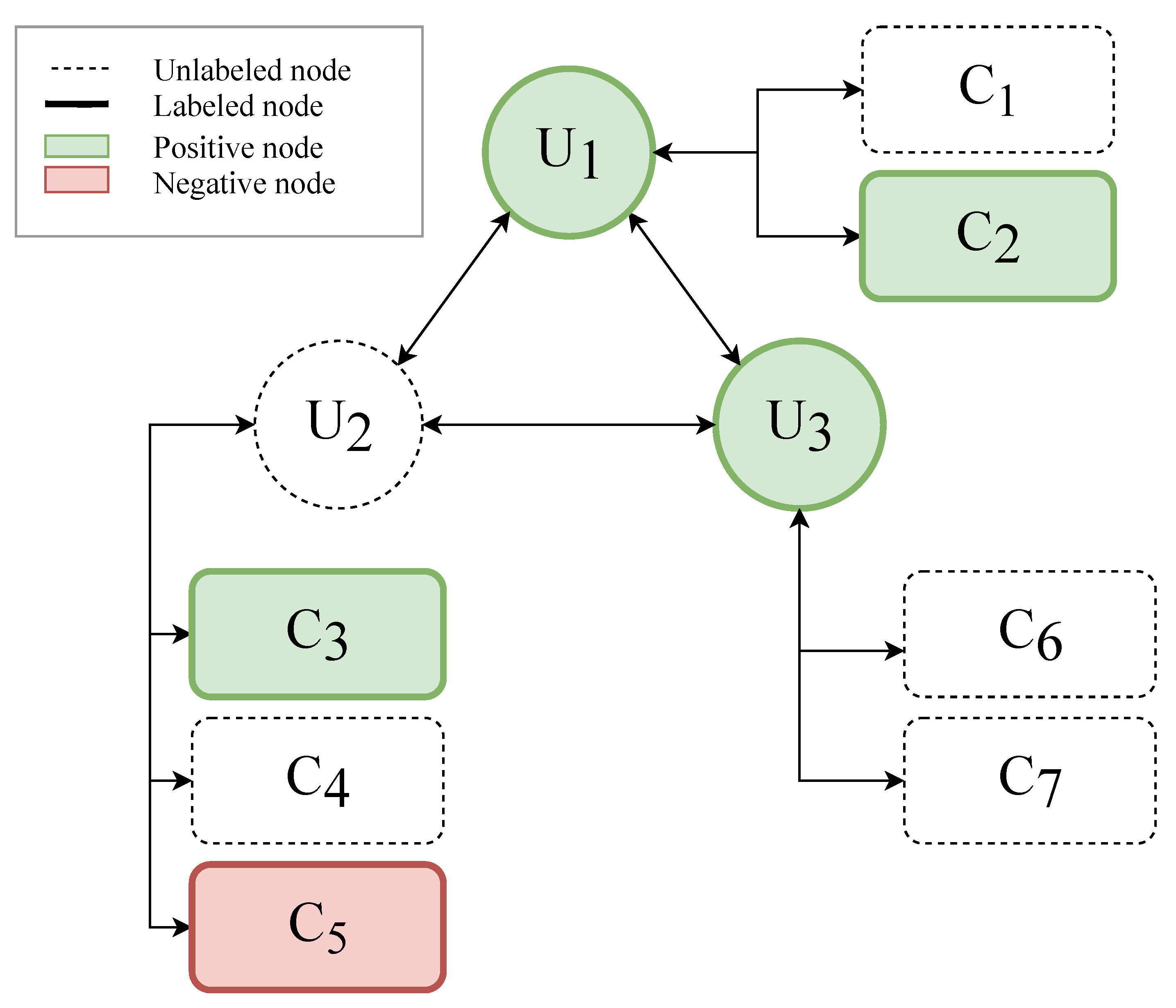
3. Sentiment Classification

The sentiment classification task consists of finding all the sentiment labels for users ($L^u=\{l_i^u\mid u_i\in U\}$) and content ($L^c=\{l_i^c\mid c_i\in C\}$) in a given social context, where the labels of a sub-set of users ($B^u$) and a sub-set of content ($B^c$) are known in advance. The social context is made up of a set of content (C), a set of users (U), relations between both users and content (R), and interactions between users and content (I). This is illustrated in Figure 2, where relations and interactions are simplified as undirected edges between nodes (i.e., users and content). For the sake of simplicity, we will only consider two possible labels: positive and negative. However, the model can be used with an arbitrary number of labels.

To solve the classification problem, we propose a classification model that uses a combination of a probability model for a given configuration of user and content labels and a classification algorithm that finds the set of labels with the highest probability. In other words, we define a metric that, based on a given social context, estimates the likelihood that users and content are labeled in a specific configuration. The metric incorporates homophily and consistency assumptions. It also involves several parameters that need to be adjusted or trained. We propose a classification method that estimates the parameters and the labels at the same time, by employing a modified version of SampleRank [35], an algorithm to estimate parameters in complex graphical models.

Both the probability model and the classification algorithm were based on two earlier works [2,32], which are described in Section 2.4. However, this section does not assume prior knowledge of these models.

3.1. Probability Model

In order to find the best configuration of user and content labels, the classification model uses a probability model that estimates the likelihood of a given distribution of user and content labels. This probability model was based on the Markov assumption that the sentiment of user $u_i$ ($l_i^u$) is influenced only by the sentiment of every piece of content $c_i$ ($l_j^c$) authored by the user ($P_i$) and the sentiment labels of its neighbors in the network ($N_i$). Likewise, the sentiment of a piece of content $c_i$ ($l_i^c$) is influenced by the sentiment label of its author. The label of a node (i.e., user or piece of content) may or may not be known in advance. If a label for a node is known, that node is said to be labeled. Labeled users ($B^u$) and content ($B^c$) are assigned a higher weight or influence on global probability.

The model is defined as follows. Let $l_i^u$ be the label for user $u_i$, and let $L^u$ be the vector of labels for all users. Let $l_i^c$ be the label for content $u_c$ and $L^c$ be the vector of labels for all content. To simplify our notation, we will also use $P_i$ as the subset of content that has been authored by user $u_i$ and $N_i$ as the subset of users who are connected to user $u_i$ in the social context graph. Two users are connected when there is an edge between them, which can be chosen from the different types of relations and interactions available in the context, i.e., $\{u_i,u_j\}\in E,E\in \{R,I\}$. The probability of a configuration of labels ($L^u,L^c$) is given by Equation (9):

$$\begin{array}{c}\hfill log\left(P(L^u,L^c)\right)=\sum _{u_i\in U}\sum _{c_j\in P_i}\mu (l_i^u,l_j^c)\frac{{\rho }_u\left(u_i\right)·{\rho }_c\left(c_j\right)}{|P_i|}\\ \hfill +\sum _{u_j\in N_i}\lambda (l_i^u,l_j^u)\frac{{\rho }_{neigh}·e_{i,j}}{\sum _{u_k\in N_i}{e}_{i,k}}\\ \hfill -log\left(Z\right)\end{array}$$

(9)

where ${\rho }_{neigh}$ is a constant that controls the weight of the effect of neighboring users, ${\rho }_u$ and ${\rho }_c$ determine the weight of each piece of content and each user, respectively, and $e_{i,j}$ is the weight of the edge between neighboring users $u_i$ and $u_j$. The value of $\mu (\alpha ,\beta )$ and $lambda(\alpha ,\beta )$ models how a node labeled $\beta$ affects a node labeled $\alpha$ ($\alpha ,\beta \in Polarities$). For the typical case, where $Polarities=\{positive,negative\}$, $\mu$ and $\lambda$ can be thought of as an array with four values, one per combination of the two polarities. For instance, the value of ${\mu }_{positive,positive}$ is the weight given to positive content by positive users.

The weight of a specific user is controlled through ${\rho }_u$ (Equation (10)), and ${\rho }_c$ (Equation (11)) controls the weight of each piece of content. The values of both functions depend on whether the label for the specific user and or content is known a priori. For users with a known sentiment, the weight is ${\rho }_{labeled}$, and for unknown values, it is ${\rho }_{unlabeled}$. Based on previous works [2,32], we use the following values: ${\rho }_{u,labeled}={\rho }_{c,labeled}=1$, ${\rho }_{u,unlabeled}={\rho }_{c,unlabeled}=0.2$Ȯnce again, $e_{i,j}$ is the weight of the edge between users $u_i$ and $u_j$. Intuitively, this allows for some specific edges to represent stronger bonds and, hence, have a bigger impact on the result. The influence of neighboring agents ${\rho }_{neigh}$ is a parameter that can be adjusted.

$${\rho }_u\left(u\right)=\left\{\begin{array}{cc}{\rho }_{u,labeled}\hfill & \hfill :\mathrm{if}u\in B^u\\ {\rho }_{u,unlabeled}\hfill & \hfill :\mathrm{otherwise}\end{array}\right\}$$

(10)

$${\rho }_c\left(c\right)=\left\{\begin{array}{cc}{\rho }_{c,labeled}\hfill & \hfill :\mathrm{if}u\in B^c\\ {\rho }_{c,unlabeled}\hfill & \hfill :\mathrm{otherwise}\end{array}\right\}$$

(11)

3.2. Parameter Estimation and Classification

Some parameters in the probability model in the previous section were manually set, such as ${\rho }_{neigh}$ or ${\rho }_{u,labeled}$, whereas other values were to be calculated. More specifically, the classification process would consist of calculating the values for $\mu$ and $\lambda$ and then maximizing the log-likelihood of a given distribution of labels ($L^u$ and $L^c$).

In order to explain the classification process, it is useful to decompose the log-likelihood into a dot product of a matrix of constants and a function of the set of labels:

$$log\left(P(L^u,L^c)\right)=\varphi ·\psi (L^u,L^c)-log\left(Z\right)$$

(12)

where $\varphi$ (Equation (13)) is constant and the value of $\psi$ (Equation (13)) only depends on the labels and the pre-set parameters. In Equation (13), the $\mu$ and $\lambda$ functions are represented as matrices, where ${\mu }_{\alpha ,\beta }=\mu (\alpha ,\beta )$. In Equation (14), we simply introduced an auxiliary function, $\gamma$ (Equation (15)), to separate the summations into components, just like $\mu$ and $\lambda$.

$$\varphi =\{\mu ,\lambda \}$$

(13)

$$\begin{array}{c}\hfill \psi (L^u,L^c)=\{\sum _{u_i\in U}\sum _{c_j\in P_i}{\gamma }_{\alpha ,\beta }(l_i^u,l_j^c)\frac{{\rho }_u\left(u_i\right)·{\rho }_c\left(c_j\right)}{|P_i|},\\ \hfill \sum _{u_i\in U}\sum _{u_j\in N_i}{\gamma }_{\alpha ,\beta }(l_i^u,l_j^u)\frac{{\rho }_{neigh}·e_{i,j}}{{\displaystyle \sum _{u_k\in N_i}}{e}_{i,k}}\}\end{array}$$

(14)

$${\gamma }_{\alpha ,\beta }(a,b)=\left\{\begin{array}{cc}1\hfill & :a=\alpha \wedge b=\beta \hfill \\ 0\hfill & :otherwise\hfill \end{array}\right\}$$

(15)

The model is thus trained by inferring the values of $\varphi$ and the Z constant. As we explained earlier, the value of $\varphi$ roughly encodes the expected likelihood of finding a given combination of labels for two nodes. For instance, ${\lambda }_{positive,positive}$ is the likelihood of positive content on positive users, which is expected to be lower than ${\lambda }_{negative,positive}$, under the assumption of consistency. Once these parameters are calculated for a given domain, the classification consists of maximizing the log-likelihood of a given distribution of labels.

SampleRank can be used to determine the value of $\varphi$, which is divided into ${\mu }_{\alpha ,\beta }$ and ${\lambda }_{\alpha ,\beta }$. Ideally, the value of Z could be obtained through regularization, but in practice, this can be costly. This need can be circumvented by using other methods that calculate the labels for all unknown elements, such as loopy belief propagation. Alternatively, some works exploit the fact that SampleRank can also output the set of labels in addition to the value for $\varphi$ [2]. When used in this manner, training can be interpreted as a search in the space of possible labels, and the log-likelihood function is a heuristic that restricts the search. This method has been used successfully for user classification [2], and its main advantage is that it is simpler than using an additional layer of label propagation.

Our proposed classification algorithm (Algorithm 1) is a modified version of SampleRank, which returns the labels for both users and content.

Algorithm 1 Sentiment detection.
Input
$B_u:\{(u,p)\mid u\in U,p\in Polarities\}$	▹ Known user labels
$B_c:\{(c,p)\mid c\in C,p\in Polarities\}$	▹ Known content labels
$E_u:\{(i,j)\mid i,j\in U\}$	▹ Edges connecting users
$E_{uc}:\{(u,c)\mid u\in U,c\in C\}$	▹ Edges between users and content
$P:L^N\to \mathbb{R}$	▹ Performance (accuracy)
$\psi :L^N\times P^N\to \mathbb{R}$	▹ Objective function
Output
$L_u$	▹ Estimated user labels
$L_c$	▹ Estimated content labels
$\varphi$	▹ Learned weights
1: $E_u\leftarrow CD\left(E_u\right)$	▹ Community detection. This is skipped in CrankNoComm
2: $L_u,L_c\leftarrow Random(L_u,L_c)$
3: $Stale\leftarrow 0$
4: for $step\leftarrow 1$ to $MaxSteps$ do
5:  $L_{unew},L_{cnew}\leftarrow Sample(L_u,L_c)$	▹ Randomly modify only one label
6:  $\nabla \leftarrow \psi (L_{unew},L_{cnew}{B}_u,B_c,E_u,E_{uc})-\psi (L_u,L_c,B_u,B_c,E_u,E_{uc})$
7: $\Delta P\leftarrow P(L_{unew},L_{cnew})-P(L_u,L_c)$
8: if $\varphi ·\nabla >0\wedge \Delta P<0$ then	▹ Performance is worse, objective is better
9:  $\varphi \leftarrow \varphi -\eta \nabla$	▹ Performance is better, objective is worse
10: else if $\varphi ·\nabla <0\wedge \Delta P>0$ then
11:  $\varphi \leftarrow \varphi +\eta \nabla$	▹ Converge if there are no changes in a given number of steps
12: if $\nabla \le 0\wedge P(L_{cnew},L_u)\le 0$ then
13:  $Stale\leftarrow Stale+1$
14:  if $Stale>=Convergence$ then return
15: else
16:  $Stale\leftarrow 0$
17: if $\Delta P>0\vee (\Delta P=0\wedge \varphi ·\nabla >0)$ then	▹ Performance is better, and objective function is at least the same
18:  $L_u\leftarrow L_{unew}$
19:  $L_c\leftarrow L_{cnew}$
20:

In this algorithm, the $Random(L_u,L_c)$ function returns a random set of user and content labels (within the range of $Polarities$, which in a simple case would just be negative and positive). $E_u$ represents edges between users, i.e., either relations or interactions. The $CD\left(E_u\right)$ function performs community detection given a set of edges and returns the set of edges between all users within the same community. In particular, we are using the Louvain method [36]. The $Sample(L_u,L_c)$ function changes one of the labels from either $L_u$ or $L_c$, at random. Since the SampleRank algorithm is inherently stochastic, the model should be run several times, and the results of each run should be aggregated. In our case, we used a number of 21 iterations, based on earlier works [32], and simple majority over all iterations.

4. Data

4.1. Datasets

Table 1. Datasets used in the experiments. OMD, Obama–McCain Debate; HCR, Health Care Reform.

	Source	Users	Entries	Year
OMD [37]	Twitter	893	1261	2009
HCR [38]	Twitter	277	1434	2011
RTMind [2]	Twitter	62	159	2013

provides basic information about the datasets used in the evaluation. Since the model used in this work requires a social context with interactions or relations, the list is limited to datasets that either contained this information or that could be extended using other sources (Section 4.2).

The OMD dataset (Obama-McCain debate) [37] contains tweets about the televised debate between Senator John McCain and then-Senator Barack Obama. The tweets were detected by following three hashtags: #current, #tweetdebate, and #debate08. The dataset contained tweets captured during the 97-minute debate, and 53 after it, for a total of 2.5 hours. The dataset included tweet IDs, publication date, text, author name and nickname, and individual annotations of up to seven annotators.

The Health Care Reform (HCR) [38] dataset contained tweets about the run-up to the signing of the health care bill in the USA on March 23, 2010. It was collected using the #hcr hashtag, from early 2010. A subset of the collected tweets were annotated with polarity (positive, negative, neutral, and irrelevant) and polarity targets (health care reform, Obama, Democrats, Republicans, Tea Party, conservatives, liberals, and Stupak) by Speriosu et al. [38]. The tweets were separated into training, dev(HCR-DEV), and test (HCR-TEST) sets. The dataset contained the tweet ID, user ID and username, text of the tweet, sentiment, target of the sentiment, and the annotator and annotator ID.

RTMind [2] contained a set of 62 users and 159 tweets, with positive or negative annotations. To collect this dataset, Pozzi et al. [2] crawled 2500 Twitter users who tweeted about Obama during two days in May 2013. For each user, their recent tweets (up to 3200, the limit of the API) were collected. At that point, only users that tweeted at least 50 times about Obama were considered. The tweets from those users that relate to Obama were kept and manually labeled by three annotators. Then, a synthetic network of following relations was generated based on a homophily criterion, i.e., users with a similar sentiment were more likely to be connected. The dataset contained the ID of the tweet, the ID of the author, the text of the tweet, the creation time, and the sentiment (positive or negative).

4.2. Gathering and Analyzing Social Context

The model proposed needs to access the network of users. Since all datasets provide both tweet and user IDs, it would be possible to access Twitter’s public API to retrieve the network. However, that approach has several disadvantages that stem from the fact that these datasets were originally captured circa 2010 [1], such as the fact that the relationships between users have likely changed and that many of the original tweets and users have been deleted or made private, making it impossible to fetch them. Alternatively, we decided to retrieve the follower network from a snapshot of the whole Twitter network in summer of 2009 [39]. Since the datasets used were gathered around the same time period as the snapshot, this should provide a more reliable list of followers than other methods. We refer to the the resulting network as relations.

Upon realizing that the relations network was rather sparse for the OMD and HCR datasets, we investigated an alternative to find hidden links between users: connecting users that followed similar people. To do so, we extracted the list of users followed by each author and we compared the list of followees for each pair of users in the dataset. Users that shared at least a given ratio of their followees were considered similar, and an edge between them was drawn. After evaluating different values for the threshold ratio, it was set to 15%, as it resulted in a degree similar to the RT Mind dataset. We refer to this network as common.

To compare the two network variants, relations and common, we used some basic statistics of each network, shown in

Table 2. Statistics of the networks gathered for each dataset.

Dataset	Variant	Content Mean	Content Median	Degree	Isolation Ratio	Majority Agreement	# Edges	# Nodes	Total Agreement	Content Label Ratio	USer Label Ratio
RT Mind	relations	2.56	3.00	8.61	0.00	0.90	267	62	0.52	0.56	0.52
OMD	relations	2.56	1.00	14.25	0.24	0.39	6364	893	0.16	0.61	0.69
	common	2.56	1.00	9.59	0.24	0.30	4280	893	0.15	0.61	0.69
HCR	relations	1.21	1.00	0.02	0.99	0.01	3	277	0.01	0.62	0.60
	common	1.21	1.00	2.89	0.80	0.19	400	277	0.18	0.62	0.60

. The table includes the average degree of each node in the network (i.e., mean number of edges per node), the ratio of users that have the same label as the majority of their neighbors in the network (majority agreement), the ratio of users that have the same label as all their neighbors (total agreement), and the ratio of users that do not have any neighbors (isolation ratio). The degree measures the density of the network. The majority and total agreement metrics are a measure of homophily in the network. The table also includes two measures of the balance in labels for user (user label ratio) and content (content label ratio). These two metrics were calculated by dividing the number of elements (i.e., users and content) with the most common label by the total number of elements.

We observed that the RT Mind dataset was the most promising of all the networks, as its labels were balanced, it had high density and homophily, higher content count per user, and all of its users were connected. The OMD networks were the densest, but their agreement was very low and a fourth of its users not connected to others. Moreover, we observed that the common extension of this dataset had a lower agreement ratio and fewer edges, whereas the isolation ratio remained the same as in the relations network. Lastly, the HCR dataset showed the lowest agreement of the datasets, and the relations network was almost non-existent. Although the common network significantly improved every metric, the majority agreement was still very low (0.29). This meant that the additional links were connecting users that were dissimilar, which negated the homophily assumption.

In summary, we concluded that this particular strategy to extend social context did not work for these datasets. The statistics for the RT Mind dataset made it ideal for the evaluation of our proposed model. The results for the OMD dataset may indicate how the model would work in scenarios with a higher degree, but relatively low homophily. In that scenario, the $meso$ features may interfere with $micro$ features. Lastly, the HCR dataset could show how the model would work with an almost complete lack of $meso$ features.

5. Evaluation

The sentiment classification task can be divided into two sub-tasks: user-level classification, which only focuses on predicting user labels ($L^u$), and content-level classification, which focuses on content labels ($L^c$). Since these two tasks are seldom tackled at the same time, we will evaluate how the model performs in each of them independently. The datasets used are described in Section 4.

First, we focus on user-level classification (Section 5.1). The main goal was to evaluate the effect of adding community detection to the SampleRank algorithm and to compare the performance of the model to others. Then, we evaluated the content-level classification (Section 5.2) with varying levels of certainty about user and content labels.

We will compare the performance of CRANKto other classifiers that will serve as the baseline and to the results of other works in the state-of-the-art. Each model will be evaluated on different scenarios, i.e., different social contexts. The ratio of labeled (i.e., known) users and content had a significant impact on the performance of the model. Thus, we evaluated each model with different ratios of known labels for both users ($rati{o}_u$) and content ($rati{o}_c$). In each scenario, a random set of labels was kept, according to $rati{o}_u$ and $rati{o}_c$. This process was repeated several times to ensure that the results were not too biased by the random partition. For each combination of $model$, $dataset$, $rati{o}_u$, and $rati{o}_c$, the results were aggregated and the mean accuracy and its standard deviation calculated. Accuracy was chosen over other metrics because it is commonly used in the field [1].

5.1. User-Level Classification

For the evaluation of user classification, we wanted to test whether Hypothesis 1 ($meso$ features improve user classification in the absence of $micro$ features) and Hypothesis 4 ($mes{o}_e$, and community detection in particular, can improve classification compared to only using $mes{o}_i$ and $mes{o}_r$ features) held true. In our case, Hypothesis 1 was tested by comparing the accuracy of the CRANK model to a simpler model that labeled each user using the majority label of his/her content. Hypothesis 4 was tested by comparing the CRANK model to CRANK without community detection.

The following models were compared:

• Average content (AvgContent) ($micro$): Content was applied the same label as the majority of content by the same user, and users were labeled according to the majority label of their content.
• Naive majority (AvgNeigh) ($mes{o}_i$ or $mes{o}_r$, depending on the context): Users were labeled with the majority label in their group of neighbors in the network. Unlabeled content was given the label of its creator.
• Majority in the community (AvgComm) ($mes{o}_e$): Users were grouped into communities, and each user was given the majority label of the users in their community. Content was given the label of its creator.
• CRANK without community detection ($mes{o}_r$ or $mes{o}_i$, depending on the context): The CRANK model described in Algorithm 1, but using original edges instead of applying community detection.
• CRANK ($mes{o}_e$): Before applying Algorithm 1, the communities between users were extracted and converted to user edges, i.e., users in the same community were connected by an edge.

The results of the evaluation are shown in

Table 3. User-level classification accuracy for each model.

Dataset	${\mathit{ratio}}_{\mathit{c}}$	Model ${\mathit{ratio}}_{\mathit{u}}$	AvgComm	AvgContent	AvgNeigh	CRANK	CrankNoComm
RT Mind	0.25	0.25	0.536	0.692	0.540	0.883	0.815
		0.50	0.661	0.670	0.651	0.950	0.939
		0.75	0.954	0.642	0.791	0.962	0.985
	0.50	0.25	0.536	0.860	0.540	0.933	0.828
		0.50	0.663	0.843	0.651	0.964	0.961
		0.75	0.951	0.861	0.791	0.965	0.985
HCR	0.25	0.25	0.597	0.713	0.597	0.681	0.660
		0.50	0.608	0.712	0.607	0.698	0.681
		0.75	0.636	0.742	0.636	0.697	0.684
	0.50	0.25	0.597	0.807	0.597	0.789	0.789
		0.50	0.610	0.816	0.610	0.795	0.791
		0.75	0.636	0.814	0.636	0.796	0.767
OMD	0.25	0.25	0.701	0.756	0.699	0.710	0.674
		0.50	0.706	0.763	0.704	0.720	0.706
		0.75	0.703	0.763	0.699	0.724	0.708
	0.50	0.25	0.702	0.811	0.700	0.712	0.684
		0.50	0.706	0.811	0.705	0.736	0.724
		0.75	0.701	0.819	0.699	0.731	0.731

, where the highest value for each row is presented in bold. It also highlights in grey the highest value when the average content was ignored.

If we focus on the results for the RT Mind dataset, we could conclude that CRANK significantly improved the classification in all scenarios, especially with lower $rati{o}_c$ values. In other datasets, where the network of users was sparser and less cohesive, CRANK outperformed all the models, except for the average of content. This was expected, since $meso$ features in these datasets were rather weak, and the content mean and median values were close to one. In particular, the difference between the CRANK model and the baseline in the HCR dataset was relatively small (0.02). That indicated that there was little penalty to using CRANK even when there were few $meso$ edges between users. In the OMD dataset, which had low agreement between neighbors, the difference between CRANK and the baseline was higher, and it did not decrease with higher values of $rati{o}_u$. This confirmed our suspicions that the $meso$ features in this dataset were not useful for our purposes.

Regarding Hypothesis 4, we observed that CRANK outperformed its variant without community detection in most of the cases. The exceptions were cases where most of the user labels were known. In those cases, the accuracy of both methods was extremely high (above 0.95). This difference could be explained by interpreting community detection as an aggregate over several users. In general, all the users in a community shared the same sentiment. However, some members would have a different label from the majority in their community (i.e., outliers). Often, those outliers were users that were connected to users of other communities with a different sentiment. That information was lost when aggregating, so for those outliers, community detection was actually detrimental. The fewer users that were left unlabeled, the higher the effect of those outliers would be. Aggregating in those cases presented a higher variance, which combined with the high accuracy values also lowered the mean compared to not aggregating. Nevertheless, we could conclude that $mes{o}_e$ features improved user classification in most cases.

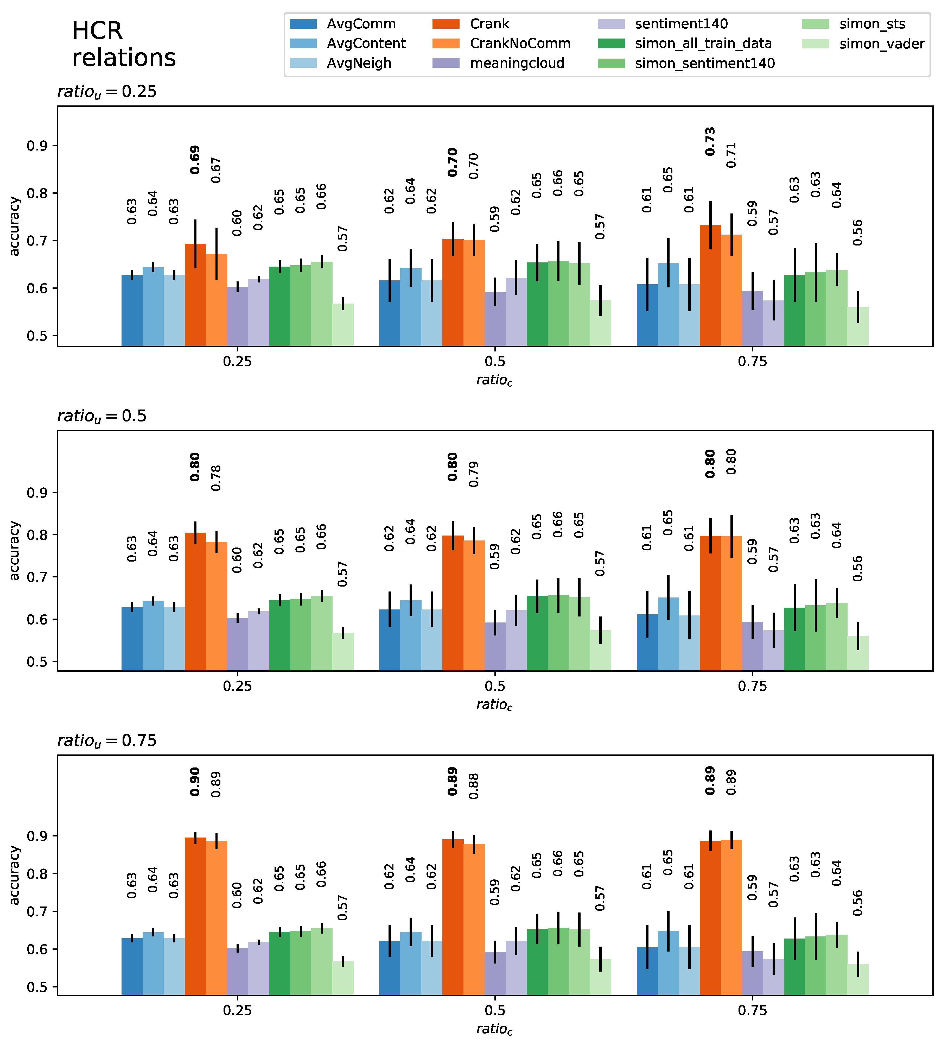
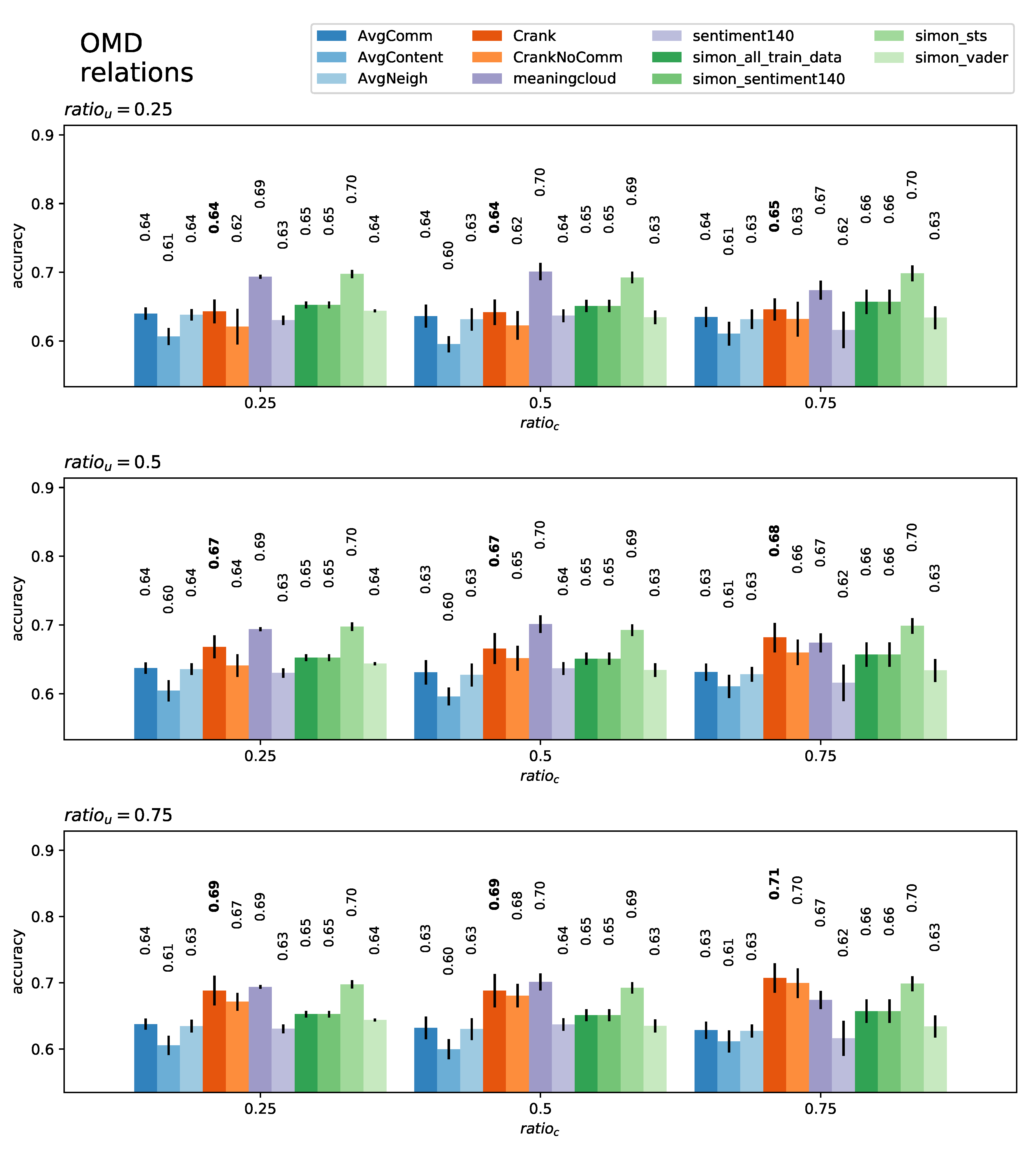
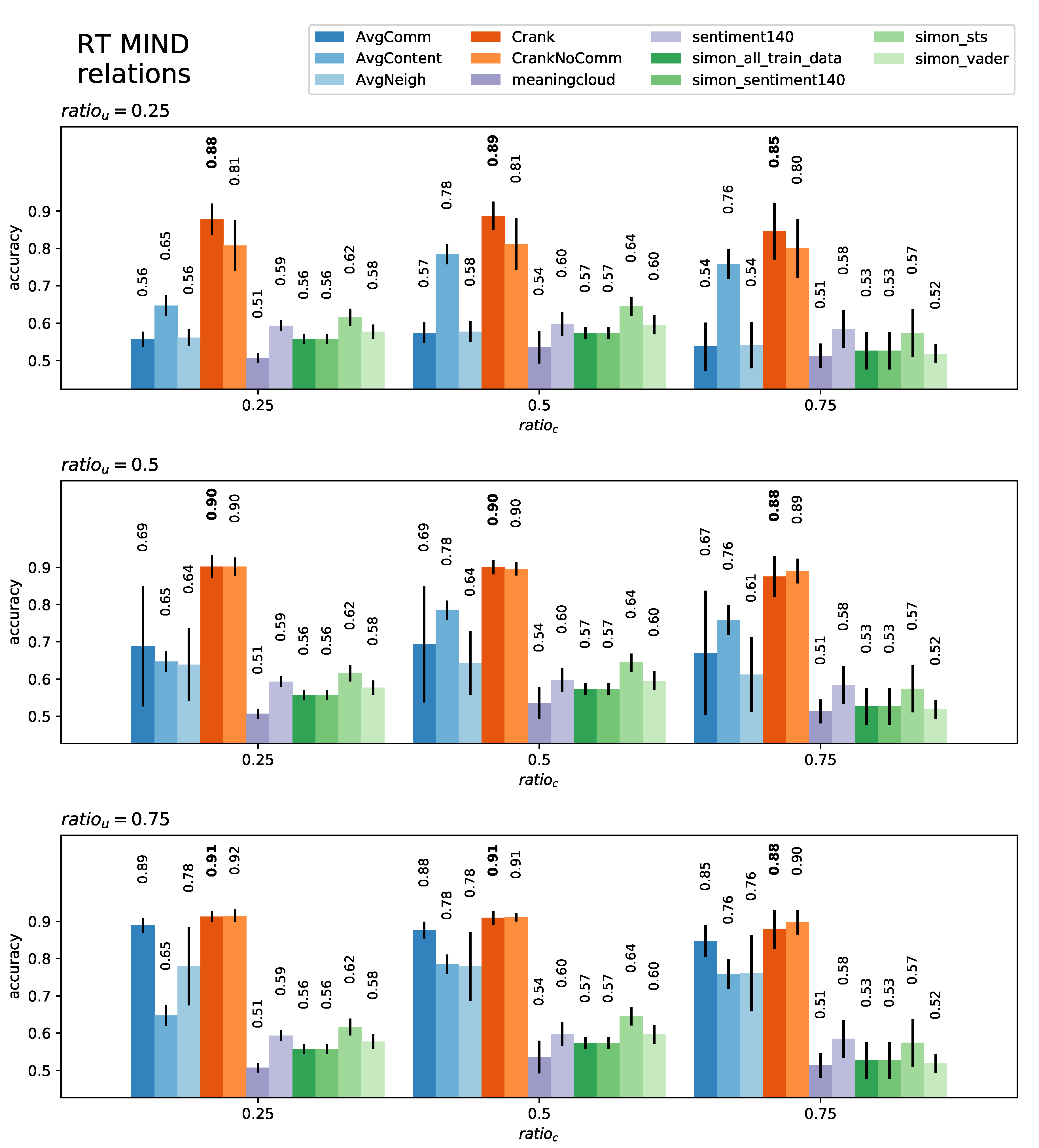
5.2. Content-Level Classification

For the evaluation of content classification, we wanted to test whether Hypothesis 2 ($micro$ features improve content classification over pure $contextless$ features), Hypothesis 3 ($meso$ features improve content classification in the absence of $micro$ features), and Hypothesis 4 ($mes{o}_e$, and community detection in particular, can improve classification compared to only using $mes{o}_i$ and $mes{o}_r$ features) held true. To do so, we compared the performance of the following classifiers:

• Simon [40] ($contextless$): A sentiment analysis model based on semantic similarity. The model can be trained with different datasets. In our evaluation, we compared with the Simon model trained on different datasets: STS, Vader, Sentiment140, and a combination of all three.
• Sentiment140 (https://www.sentiment140.com) service ($contextless$): This is a public sentiment analysis service, tailored to Twitter. It outputs three labels: positive, negative, and neutral. This results in lower accuracy for the negative and positive labels. In fact, of all the models tested, this was the one with the lowest accuracy. If all tweets labeled neutral by the service are ignored, its accuracy reaches standard levels (around 60%). Unfortunately, this means that around 80% of tweets have to be ignored.
• Meaningcloud (https://www.meaningcloud.com/) Sentiment Analysis ($contextless$): An enterprise service that provides several types of text analysis, including sentiment analysis. It poses the same restrictions for evaluation as Sentiment140, as it provides positive, negative, and neutral labels. Fortunately, the subjectivity detection of this service for our datasets was better than that of Sentiment140.
• Average Content (AvgContent) ($micro$): Content is applied the same label as the majority of content by the same user, and users are labeled according to the majority label of their content.
• Naive majority (AvgNeigh) ($mes{o}_i$ or $mes{o}_r$, depending on the context): Users are labeled with the majority label in their group of neighbors in the network. Unlabeled content is given the label of its creator.
• Majority in the community (AvgComm) ($mes{o}_e$): Users are grouped into communities, and each user is given the majority label of the users in their community. Content is given the label of its creator.
• CRANK without community detection ($mes{o}_r$ or $mes{o}_i$, depending on the context): The CRANK model described in Algorithm 1, but using original edges instead of applying community detection.
• CRANK ($mes{o}_e$): Before applying Algorithm 1, the communities between users are extracted and converted to user edges, i.e., users in the same community are connected by an edge.
• Label propagation [38] (Speriosu): Based on the results reported in the original paper for these datasets.

We compared the accuracy of each of these models for several combinations of known content and user labels ($rati{o}_c$ and $rati{o}_u$).

Table 4. Content-level classification accuracy of each model.

Dataset	${\mathit{ratio}}_{\mathit{u}}$	Algo ${\mathit{ratio}}_{\mathit{c}}$	AvgComm	AvgContent	AvgNeigh	CRANK	CrankNoComm	Meaningcloud	Sentiment140	Simon_All_Train_Data	Simon_Sentiment140	Simon_sts	Simon_Vader
RT Mind	0.25	0.25	0.56	0.65	0.56	0.88	0.81	0.51	0.59	0.56	0.56	0.62	0.58
		0.50	0.57	0.78	0.58	0.89	0.81	0.54	0.60	0.57	0.57	0.64	0.60
		0.75	0.54	0.76	0.54	0.85	0.80	0.51	0.58	0.53	0.53	0.57	0.52
	0.50	0.25	0.69	0.65	0.64	0.90	0.90	0.51	0.59	0.56	0.56	0.62	0.58
		0.50	0.69	0.78	0.64	0.90	0.90	0.54	0.60	0.57	0.57	0.64	0.60
		0.75	0.67	0.76	0.61	0.88	0.89	0.51	0.58	0.53	0.53	0.57	0.52
	0.75	0.25	0.89	0.65	0.78	0.91	0.92	0.51	0.59	0.56	0.56	0.62	0.58
		0.50	0.88	0.78	0.78	0.91	0.91	0.54	0.60	0.57	0.57	0.64	0.60
		0.75	0.85	0.76	0.76	0.88	0.90	0.51	0.58	0.53	0.53	0.57	0.52
HCR	0.25	0.25	0.63	0.64	0.63	0.69	0.67	0.60	0.62	0.65	0.65	0.66	0.57
		0.50	0.62	0.64	0.62	0.70	0.70	0.59	0.62	0.65	0.66	0.65	0.57
		0.75	0.61	0.65	0.61	0.73	0.71	0.59	0.57	0.63	0.63	0.64	0.56
	0.50	0.25	0.63	0.64	0.63	0.80	0.78	0.60	0.62	0.65	0.65	0.66	0.57
		0.50	0.62	0.64	0.62	0.80	0.79	0.59	0.62	0.65	0.66	0.65	0.57
		0.75	0.61	0.65	0.61	0.80	0.80	0.59	0.57	0.63	0.63	0.64	0.56
	0.75	0.25	0.63	0.64	0.63	0.90	0.89	0.60	0.62	0.65	0.65	0.66	0.57
		0.50	0.62	0.64	0.62	0.89	0.88	0.59	0.62	0.65	0.66	0.65	0.57
		0.75	0.61	0.65	0.61	0.89	0.89	0.59	0.57	0.63	0.63	0.64	0.56
OMD	0.25	0.25	0.64	0.61	0.64	0.64	0.62	0.69	0.63	0.65	0.65	0.70	0.64
		0.50	0.64	0.60	0.63	0.64	0.62	0.70	0.64	0.65	0.65	0.69	0.63
		0.75	0.64	0.61	0.63	0.65	0.63	0.67	0.62	0.66	0.66	0.70	0.63
	0.50	0.25	0.64	0.60	0.64	0.67	0.64	0.69	0.63	0.65	0.65	0.70	0.64
		0.50	0.63	0.60	0.63	0.67	0.65	0.70	0.64	0.65	0.65	0.69	0.63
		00.75	0.63	0.61	0.63	0.68	0.66	0.67	0.62	0.66	0.66	0.70	0.63
	0.75	00.25	0.64	0.61	0.63	0.69	0.67	0.69	0.63	0.65	0.65	0.70	0.64
		00.50	0.63	0.60	0.63	0.69	0.68	0.70	0.64	0.65	0.65	0.69	0.63
		00.75	0.63	0.61	0.63	0.71	0.70	0.67	0.62	0.66	0.66	0.70	0.63

shows a summary of the mean accuracy for each combination. We also provide a graph of the mean accuracy and standard deviation of each model (Figure 3, Figure 4 and Figure 5).

Similarly to the user-classification case, if we focus on the RT Mind dataset, the CRANK algorithm outperformed all other models by a wide margin. In general, the baseline models that used social context had higher accuracy in this dataset than any contextlessapproach. This was more obvious when either more content was known (better $micro$ features) or more users were known (better $meso$ features). This evidence supported Hypotheses 2 and 3.

In this case, averaging the content of a user yielded poor results for all datasets, due to the low content count per user. If we look at all the results, we observe once again that the version of CRANK with community detection had consistently better accuracy, supporting Hypothesis 4. It should be noted that the Simon model [40] achieved the best performance among the contextless models and the overall best in the OMD dataset. Unfortunately, the results for that dataset were very similar for all the models, and the margins were small, so we could not draw any conclusions from that dataset.

5.3. Statistical Analysis

In order to assess the value of the comparison of the models, a statistical test was performed on the experimental results. More specifically, we used a combination of Friedman’s test with the corresponding Bonferroni–Dunn post-hoc test, which is oriented toward the comparison of several classifiers on multiple datasets [41].

First of all, in Section 5.1, we claimed that the version of CRANK with community detection outperformed the version without it. To assess that claim, we compared all the user and content-level classification cases for both models. Friedman’s test revealed the difference between both models was statistically different, with a chi-squared of 104 and a p-value of $2.9e^{-5}$. The post-hoc Bonferroni–Dunn test also passed with a calculated difference of 0.63, which was above a critical difference of 0.27.

Secondly, we compared all the user-level models, ignoring the Average Content classifier. In that case, Friedman’s test also rejected the null hypothesis, with a chi-squared of 27.4 and a p-value of $0.0006$. In this case, we performed the Bonferroni–Dunn test, with the average of neighbors as the baseline, and both CRANK and CRANK without communities passed it. The results for average in community and average of neighbors were not conclusive.

Secondly, we performed a similar comparison for content-level classification. We compared the following approaches to the Sentiment140 baseline. The calculated critical difference for this case was $3.299$. The results were that only CRANK, CRANK without communities, and Simon trained with the STS dataset were better than the baseline (

Table 5. Ranking from Friedman’s test in content-level classification.

	sentiment140	AvgContent	CRANK	CrankNoComm	Speriosu	meaningcloud	simon_all_train_data	simon_sentiment140	simon_sts	simon_vader
Pass	Baseline	No	Yes	Yes	No	No	No	No	Yes	No
Diff.	0.0	0.81	4.96	4.04	1.52	0.56	0.85	1.19	3.52	−1.0

). Unfortunately, we could not reject the null hypothesis for CRANK and Simon STS alone at the desired level of confidence, given the number of datasets. Nevertheless, if we reduced our test to the scenarios with the RT Mind dataset at different ratios of $r_u$ and $r_c$, the null hypothesis could be rejected with $\alpha =0.1$.

6. Conclusions and Future Work

In this work, we proposed a model that united features from different levels of social context ($micro$, $meso$, and $mes{o}_e$). This model was an extension of earlier models that were limited to user-level classification. Moreover, it employed community detection, which found weak relationships between users that were not directly connected in the network. We expected the combination to have an advantage at different levels of certainty about the labels in the context and with varying degrees of sparsity in the social network. The proposed model was shown to work for both types of classification in different scenarios.

To evaluate the model, we looked at different datasets. The need for a social context restricted the number of datasets that could be used in the evaluation. Of the three datasets included, the RT Mind dataset seemed to be the most appropriate, as it contained a more densely connected network of users. The results of evaluating CRANK with other baseline models in that dataset provided limited support for Hypothesis 4 ($mes{o}_e$ features improve user classification). Moreover, the evidence from evaluating all the datasets supported Hypotheses 2 ($micro$ features improve content classification) and 3 ($meso$ features improve content classification). By comparing the two versions of CRANK (with and without community detection) in both user- and content-level classification, we also validated Hypothesis 4 ($mes{o}_e$ features improve user and content classification). Nonetheless, the analysis of the datasets in Section 4.2 revealed the need for better datasets, which could be enriched with context, i.e., datasets with inter-connected users and more content per user. Hence, further evaluation would be needed, once richer datasets become available.

In addition to evaluating more domains and datasets, there are several lines of future research. In this work, we used a random user and content selection strategy to generate the evaluation datasets. A random sampling strategy for users and content led to higher sparsity. Since the performance of the model depended on having a densely connected graph, it would be interesting to evaluate the effect of different sampling algorithms, such as random walk, breadth-first search, and depth-first search. In particular, Breadth-First Search (BFS) sampling may be more appropriate for this scenario [42].

It would also be interesting to analyze different community detection strategies. The simplest improvement in this regard would be using other community detection algorithms. There are several methods that produce overlapping partitions, which may help alleviate the negative effect of users in the edge of two communities. More sophisticated strategies are also possible, such as automatically deciding to apply community detection based on the network and the ratio of known users or only adding edges for some users.

References

1. Sánchez-Rada, J.F.; Iglesias, C.A. Social Context in Sentiment Analysis: Formal Definition, Overview of Current Trends and Framework for Comparison. Inf. Fus. 2019. [Google Scholar] [CrossRef]
2. Pozzi, F.A.; Maccagnola, D.; Fersini, E.; Messina, E. Enhance user-level sentiment analysis on microblogs with approval relations. In Proceedings of the Congress of the Italian Association for Artificial Intelligence; Springer: Turin, Italy, 2013; pp. 133–144. [Google Scholar]
3. Pang, B.; Lee, L. Opinion Mining and Sentiment Analysis. Found. Trends® Inf. Retr. 2008, 2, 1–135. [Google Scholar] [CrossRef] [Green Version]
4. Ravi, K.; Ravi, V. A survey on opinion mining and sentiment analysis: Tasks, approaches and applications. Knowl.-Based Syst. 2015, 89, 14–46. [Google Scholar] [CrossRef]
5. Sharma, A.; Dey, S. A comparative study of feature selection and machine learning techniques for sentiment analysis. In Proceedings of the 2012 ACM Research in Applied Computation Symposium; ACM: New York, NY, USA, 2012; pp. 1–7. [Google Scholar]
6. Taboada, M.; Brooke, J.; Tofiloski, M.; Voll, K.; Stede, M. Lexicon-Based Methods for Sentiment Analysis. Comput. Linguist. 2011, 37, 267–307. [Google Scholar] [CrossRef]
7. García-Pablos, A.; Cuadros Oller, M.; Rigau Claramunt, G. A comparison of domain-based word polarity estimation using different word embeddings. In Proceedings of the Tenth International Conference on Language Resources and Evaluation, Portoroz, Slovenia, 23–28 May 2016. [Google Scholar]
8. Cambria, E. Affective computing and sentiment analysis. IEEE Intell. Syst. 2016, 31, 102–107. [Google Scholar] [CrossRef]
9. Kiritchenko, S.; Zhu, X.; Mohammad, S.M. Sentiment Analysis of Short Informal Texts. J. Artif. Intell. Res. 2014, 50, 723–762. [Google Scholar] [CrossRef]
10. Melville, P.; Gryc, W.; Lawrence, R.D. Sentiment Analysis of Blogs by Combining Lexical Knowledge with Text Classification. In Proceedings of the 15th ACM SIGKDD International Conference on Knowledge Discovery and Data Mining; ACM: New York, NY, USA, 2009; pp. 1275–1284. [Google Scholar]
11. Nasukawa, T.; Yi, J. Sentiment Analysis: Capturing Favorability Using Natural Language Processing. In Proceedings of the 2Nd International Conference on Knowledge Capture; ACM: New York, NY, USA, 2003; pp. 70–77. [Google Scholar]
12. Araque, O.; Corcuera-Platas, I.; Sánchez-Rada, J.F.; Iglesias, C.A. Enhancing Deep Learning Sentiment Analysis with Ensemble Techniques in Social Applications. Expert Syst. Appl. 2017, 77, 236–246. [Google Scholar] [CrossRef]
13. Pang, B.; Lee, L.; Vaithyanathan, S. Thumbs Up?: Sentiment Classification Using Machine Learning Techniques. In Proceedings of the ACL-02 Conference on Empirical Methods in Natural Language Processing; Association for Computational Linguistics: Stroudsburg, PA, USA, 2002; Volume 10, pp. 79–86. [Google Scholar]
14. Wang, S.; Manning, C.D. Baselines and Bigrams: Simple, Good Sentiment and Topic Classification. In Proceedings of the 50th Annual Meeting of the Association for Computational Linguistics: Short Papers; Association for Computational Linguistics: Stroudsburg, PA, USA, 2012; pp. 90–94. Volume 2. [Google Scholar]
15. Jiang, F.; Liu, Y.Q.; Luan, H.B.; Sun, J.S.; Zhu, X.; Zhang, M.; Ma, S.P. Microblog sentiment analysis with emoticon space model. J. Comput. Sci. Technol. 2015, 30, 1120–1129. [Google Scholar] [CrossRef]
16. Hogenboom, A.; Bal, D.; Frasincar, F.; Bal, M.; De Jong, F.; Kaymak, U. Exploiting Emoticons in Polarity Classification of Text. J. Web Eng. 2015, 14, 22–40. [Google Scholar]
17. Novak, P.K.; Smailović, J.; Sluban, B.; Mozetič, I. Sentiment of emojis. PLoS ONE 2015, 10, e0144296. [Google Scholar]
18. Collobert, R.; Weston, J.; Bottou, L.; Karlen, M.; Kavukcuoglu, K.; Kuksa, P. Natural language processing (almost) from scratch. J. Mach. Learn. Res. 2011, 12, 2493–2537. [Google Scholar]
19. Bengio, Y. Learning Deep Architectures for AI. Found. Trends® Mach. Learn. 2009, 2, 1–127. [Google Scholar] [CrossRef]
20. Marcus, G. Deep learning: A critical appraisal. arXiv 2018, arXiv:1801.00631. [Google Scholar]
21. Lipton, Z.C. The mythos of model interpretability. arXiv 2016, arXiv:1606.03490. [Google Scholar] [CrossRef]
22. Kim, Y. Convolutional neural networks for sentence classification. arXiv 2014, arXiv:1408.5882. [Google Scholar]
23. Mikolov, T.; Chen, K.; Corrado, G.; Dean, J. Efficient estimation of word representations in vector space. arXiv 2013, arXiv:1301.3781. [Google Scholar]
24. Otte, E.; Rousseau, R. Social network analysis: a powerful strategy, also for the information sciences. J. Inf. Sci. 2002, 28, 441–453. [Google Scholar] [CrossRef]
25. Sixto, J.; Almeida, A.; López-de Ipiña, D. Analysis of the Structured Information for Subjectivity Detection in Twitter. In Proceedings of the Transactions on Computational Collective Intelligence XXIX, Bristol, UK, 5–7 September 2018; pp. 163–181. [Google Scholar]
26. Hajian, B.; White, T. Modelling Influence in a Social Network: Metrics and Evaluation. In Proceedings of the 2011 IEEE Third International Conference on Privacy, Security, Risk and Trust and 2011 IEEE Third International Conference on Social Computing, Security, Boston, MA, USA, 9–11 October 2011; pp. 497–500. [Google Scholar]
27. Noro, T.; Tokuda, T. Searching for Relevant Tweets Based on Topic-related User Activities. J. Web Eng. 2016, 15, 249–276. [Google Scholar]
28. Papadopoulos, S.; Kompatsiaris, Y.; Vakali, A.; Spyridonos, P. Community detection in social media. Data Min. Knowl. Discov. 2012, 24, 515–554. [Google Scholar] [CrossRef]
29. Deitrick, W.; Hu, W. Mutually Enhancing Community Detection and Sentiment Analysis on Twitter Networks. J. Data Anal. Inf. Process. 2013, 01, 19–29. [Google Scholar] [CrossRef] [Green Version]
30. Gao, B.; Berendt, B.; Clarke, D.; De Wolf, R.; Peetz, T.; Pierson, J.; Sayaf, R. Interactive grouping of friends in OSN: Towards online context management. In Proceedings of the 2012 IEEE 12th International Conference on Data Mining Workshops (ICDMW), Brussels, Belgium, 10 December 2012; pp. 555–562. [Google Scholar]
31. Orman, G.K.; Labatut, V.; Cherifi, H. Qualitative comparison of community detection algorithms. In Proceedings of the 2011 International Conference on Digital Information and Communication Technology and Its Applications, Bangkok, Thailand, 21–23 June 2011; pp. 265–279. [Google Scholar]
32. Tan, C.; Lee, L.; Tang, J.; Jiang, L.; Zhou, M.; Li, P. User-level Sentiment Analysis Incorporating Social Networks. In Proceedings of the 17th ACM SIGKDD International Conference on Knowledge Discovery and Data Mining; ACM: New York, NY, USA, 2011; pp. 1397–1405. [Google Scholar]
33. Hu, X.; Tang, L.; Tang, J.; Liu, H. Exploiting Social Relations for Sentiment Analysis in Microblogging. In Proceedings of the Sixth ACM International Conference on Web Search and Data Mining; ACM: New York, NY, USA, 2013; pp. 537–546. [Google Scholar]
34. Xiaomei, Z.; Jing, Y.; Jianpei, Z.; Hongyu, H. Microblog sentiment analysis with weak dependency connections. Knowl.-Based Syst. 2018, 142, 170–180. [Google Scholar] [CrossRef]
35. Wick, M.L.; Rohanimanesh, K.; Bellare, K.; Culotta, A.; McCallum, A. SampleRank: Training Factor Graphs with Atomic Gradients; ICML: Vienna, Austria, 2011; Volume 5, p. 1. [Google Scholar]
36. Blondel, V.D.; Guillaume, J.L.; Lambiotte, R.; Lefebvre, E. Fast unfolding of communities in large networks. J. Stat. Mech. 2008, 2008, P10008. [Google Scholar] [CrossRef] [Green Version]
37. Shamma, D.A.; Kennedy, L.; Churchill, E.F. Tweet the Debates: Understanding Community Annotation of Uncollected Sources. In Proceedings of the First SIGMM Workshop on Social Media; ACM: New York, NY, USA, 2009; pp. 3–10. [Google Scholar]
38. Speriosu, M.; Sudan, N.; Upadhyay, S.; Baldridge, J. Twitter Polarity Classification with Label Propagation over Lexical Links and the Follower Graph. In Proceedings of the Conference on Empirical Methods in Natural Language Processing; Association for Computational Linguistics: Stroudsburg, PA, USA, 2011; pp. 53–56. [Google Scholar]
39. Kwak, H.; Lee, C.; Park, H.; Moon, S. What is Twitter, a Social Network or a News Media? In Proceedings of the 19th International Conference on World Wide Web; ACM: New York, NY, USA, 2010; pp. 591–600. [Google Scholar]
40. Araque, O.; Zhu, G.; Iglesias, C.A. A semantic similarity-based perspective of affect lexicons for sentiment analysis. Knowl.-Based Syst. 2019, 165, 346–359. [Google Scholar] [CrossRef]
41. Demšar, J. Statistical comparisons of classifiers over multiple data sets. J. Mach. Learn. Res. 2006, 7, 1–30. [Google Scholar]
42. West, R.; Paskov, H.S.; Leskovec, J.; Potts, C. Exploiting Social Network Structure for Person-to-Person Sentiment Analysis. Trans. Assoc. Comput. Linguist. 2014, 2, 297–310. [Google Scholar] [CrossRef]
Figure 1. Model of social context, including: content (C), users (U), relations ( R c , R u , and R u c ), and interactions ( I u and I u c ).
Applsci 10 01662 g001
Figure 2. Problem definition. The task is to predict the missing labels.
Applsci 10 01662 g002
Figure 3. Content-level classification mean accuracy and standard deviation in the HCR dataset for each model at each level of certainty ( r a t i o u and r a t i o c ).
Applsci 10 01662 g003
Figure 4. Content-level classification mean accuracy and standard deviation in the OMD dataset for each model at each level of certainty ( r a t i o u and r a t i o c ).
Applsci 10 01662 g004
Figure 5. Content-level classification mean accuracy and standard deviation in the RT Mind dataset for each model at each level of certainty ( r a t i o u and r a t i o c ).
Applsci 10 01662 g005