Article

Analysis of Movement Law and Influencing Factors of Hill-Drop Fertilizer Based on SPH Algorithm

College of Engineering, China Agricultural University, Beijing 100083, China
*
Author to whom correspondence should be addressed.
Appl. Sci. 2020, 10(5), 1643; https://doi.org/10.3390/app10051643
Submission received: 23 December 2019 / Revised: 24 February 2020 / Accepted: 26 February 2020 / Published: 1 March 2020

Abstract

:
Studying the movement law and influencing factors of fertilizer in soil and controlling fertilizer distribution can improve the quality of fertilization, which is of great significance for promoting crop yield. In this paper, a 3D simulation model of the hill-drop fertilizer device and soil was established by the Smoothed Particle Hydrodynamics (SPH) algorithm, and the simulation model was modified using the Mohr–Coulomb criterion, and fertilizer movement in the soil under the disturbance of the cover was simulated and analyzed by the SPH algorithm. Orthogonal simulation experiments and the range analysis method were used to study the overall displacement and deformation of fertilizer, and the key factors affecting fertilizer movement were analyzed. After fertilization, the soil was layered with a soil sampler, and a digital image processing method was used to detect the fertilizer distribution in different soil depths; then, the fertilizer movement was inferred. The results of the field experiment showed that the trend of fertilizer movement was consistent with the results of the simulation experiment, which provides a reference for studying the movement and distribution of fertilizer in soil.

1. Introduction

The large-scale use of chemical fertilizer is the main way to increase grain production. Chemical fertilizer accounts for about 40%–60% of total increase in crop production. In China, the application rate of chemical fertilizer is high, and the effective utilization rate is low. The scientific application of fertilizer is an important part of conservation tillage, and it plays an important role in improving soil properties and crop yield and quality [1,2]. High-quality fertilization is an effective way to solve current soil environmental problems, and it is of great significance for achieving the comprehensive agricultural goals of high yield, fine quality, and soil amelioration [3].
Hill-drop fertilizer is in line with the law of corn growth and is an important method of scientific fertilization. Hill-drop fertilizer is a one-time application of all the fertilizer required for crop growth at the seedling stage. Compared with the furrow application method, it can improve fertilizer utilization rate and reduce environmental pollution. Scholars have carried out a series of studies on hill-drop fertilization technology. For example, Wu et al. [4] designed a hill-drop fertilizer system using a no-tillage planter, Liu et al. [5] designed a corn hill-drop fertilizer device, and Li et al. [6] designed a hill-drop fertilizer mechanism for the corn seedling stage. At present, the hill-drop fertilizer technology made great progress, and scholars made several different prototypes and tested fertilization effects. The test of fertilization effects was mainly carried out through field experiments. The research on the hill-drop fertilizer device was mainly focused on these aspects, and none of the relevant studies eamined the law of fertilizer movement.
Due to the complex soil composition, it is difficult to directly observe the fertilizer distribution. Modeling and simulation methods have been used to study the movement and distribution of soil and fertilizer. For example, Mouazen et al. [7] developed a three-dimensional model, and studied the influence of the geometric parameters of subsoiler on its performance in nonhomegeneous soils using the Finite Element Method (FEM). Shmulevich et al. [8] studied the modeling of soil-tillage interaction using the Discrete Element Method (DEM). Ucgul et al. [9] studied soil movement when disturbed by plowing using soil bin tests and a discrete element method model. Barr et al. [10] studied the process of soil disturbance and destruction using the discrete element method and a hysteretic spring contact model. Wang et al. [11] simulated the movement of fertilizer particles in a fertilizer applicator using the discrete element method.
With the improvement of the soil constitutive model and the development of the Smoothed Particle Hydrodynamics (SPH) algorithm, the SPH algorithm is gradually being applied to study the interaction between working parts and soil. For example, Gao et al. [12] studied the process of soil-cutting at high speed using the SPH algorithm, and analyzed the principle of the soil-machine system. Pastor et al. [13] used the SPH algorithm to discretize a depth-integrated, coupled solid model, and analyzed flow-like slope movements. The SPH algorithm was also used in related research studying fertilizer distribution. Zhang et al. [14] studied fertilizer distribution after fertilizer being applied to the soil using the SPH algorithm. Therefore, it was feasible to study the movement law of hill-drop fertilizer in the soil under the interaction of working parts using the SPH algorithm.
At present, there are few articles about the fertilizer movement law in soil and its influencing factors. Field experiments are mostly used for the method of detecting fertilizer. The experiment process is tedious, the workload is heavy, the interior of the soil is not easy to observe, and it is difficult to get ideal results [15]. At present, there are some limitations in the simulation methods mostly used. The finite element method is not suitable for studies with large dispersion, significant deformation, etc. The discrete element method requires high calculation speed, and the selection of the contact model parameters requires a great deal of experience [12]. Compared with other simulation methods, the SPH algorithm can better solve problems such as complex soil composition because it has no mesh distortion and less intervention of human factors, asa well as displaying higher accuracy.
There are two prominent problems in the actual application of hill-drop fertilization: one is insufficient fertilization depth, and the other is the easy accumulation of fertilizer. Both are caused by the fertilizer movement in the soil, making the actual fertilization depth less than the theoretical requirement. Fertilizer cannot be fully utilized, and sufficient nutrients are not obtained in the early stages of plants’ growth, which affects crop yield and causes environmental pollution [14].
In order to solve the problems of insufficient fertilization depth and easy accumulation of fertilizer, and to improve the qualification rate of fertilization, a hill-drop fertilizer device was designed, and a 3D model of the hill-drop fertilizer device and soil was established by the SPH algorithm in this paper. The disturbance process of fertilizer in the soil under the action of the designed cover was simulated and analyzed. The fertilizer movement law, as well as the effect on fertilization quality, were studied. Through the simulation based on the SPH algorithm, studying the movement law and influencing factors of fertilizer in the soil can provide a scientific reference for solving problems such as fertilizer accumulation, and provide a theoretical basis for improving the hill-drop fertilizer device and the fertilization quality.

2. Methodology

2.1. Hill-Drop Fertilizer Device

The corn hill-drop fertilizer planter was mainly composed of the fertilizer unit, seeding unit, land wheel transmission system, frame, and speed measuring device. As shown in Figure 1, this is the overall structure of the planter. The hill-drop fertilizer device was a key component of the fertilizer unit, and also an important part of the simulation model in this paper. It is mainly composed of an opener, an intermittent fertilizer feeder, and two covers.
When the planter was working, the fertilizer in the fertilizer box was continuously and evenly dropped along the fertilizer pipe driven by the land wheel. It was intermittently discharged through the fertilizer feeder and applied to different depths of the fertilizer ditch. It symmetrically distributed cover soil on both sides, and quickly backfilled the opened fertilizer ditch to prevent fertilizer accumulation. The speed measuring device measured the working distance of the planter and fed it back to the control system, and discharged the fertilizer evenly.

2.2. Fertilizer Motion Simulation

Soil is an unsaturated multiphase system with a complicated constitutive relationship, and soil disturbance is large when soil is furrowed by agricultural machinery. The finite element method is prone to cause mesh distortion and lower accuracy. SPH is a meshless algorithm that has been gradually developed in the last 20 years. Because the SPH algorithm does not need to define mesh, it can avoid mesh distortion and accuracy damage caused by large deformation, and it can effectively deal with problems such as soil multiphase, looseness and dispersed physical properties [16,17]. Previous studies have proven that SPH can solve fluent problems effectively, such as free surface flow [18,19] and bubble rising [20,21]. The process of disturbing soil can be seen as the flow of soil particles, and, therefore, SPH should be an effective method for simulating disturbance processes.
The kernel approximation and particle approximation are two very important steps in the SPH method [22]. To correctly characterize particle motion, an approximate function is needed to characterize particle motion information. The integral expression of the SPH function f ( x ) can be expressed as a discretized form that supports the summation of all particles in the domain [23,24]:
f ( x i ) = j = 1 n m j p j f x i W x x j , h
The function expression of the i-th particle is:
f x i = j = 1 n m j p j f x x i W x x j , h
In the formula, h is the particle smooth length in the W influence domain; m j is the particle mass; p j is the particle density; and n is the total number of particles in the support domain.
In this work, we chose the cubic spline function [25], which closely resembles a Gaussian function [26], as our smoothing function. It is defined using an auxiliary function θ x :
W ( x , h ) = 1 h ( x ) v θ ( x )
In the formula, W is the smooth kernel function (interpolation kernel), v is the space dimension, and H is the particle smooth length.
The expression of the cubic B-spline kernel function is:
θ ( u ) = 1 1.5 u 2 + 0.75 u 3 C 0 < | u | 1 0.25 C ( 2 u ) 3 1 < | u | < 2 0 2 | u |
In the formula, C is a constant and is determined by the space dimension.
The particle smooth length has a significant impact on efficiency and calculation accuracy [27]. The fixed smooth length can cause problems, such as numerical distortion and compression instability. The variable smooth length can keep the same number of particles in the domain. The range of variation is:
h min h 0 < h < h max h 0
In the formula, h 0 is the initial smooth length. The value of the smoothing length is chosen based on actual problems. The smooth length is between 0.2 and 2 times the initial smooth length, which can meet most requirements [22]. In this study, we chose 1.5 times particle spacing as the smoothing length.
The SPH algorithm discretizes a continuum into an interactive particles, and applies speed, displacement and other physical quantities to each particle. The mechanical behavior of the overall system can be obtained by tracking the motion trail of each particle [28,29,30].
In view of problems such as easy concentration of fertilizer and insufficient fertilization depth due to fertilizer movement, the designed hill-drop fertilizer device was modeled, and the disturbance process of fertilizer in the soil was simulated by the cover. The simulation model mainly included opener, cover, fertilizer, and soil.
Because of the complex structure of the hill-drop fertilizer device, the indirect modeling method was chosen in ANYSYS/LS-DYNA. A parametric solid model of cover and opener was established, and a soil model of 1000 mm × 400 mm × 400 mm also was established in CREO. The model was imported into the preprocessor and meshed. The opener used an automatic meshing method, and the mesh size was 0.05 m; the cover used an automatic meshing method, and the mesh size was 0.03 m; the soil was divided by sweep, and the mesh size was 0.01 m.
Because the soil is not a homogeneous material, the deviation between simulation results and actual values will be large if the soil is idealized as a continuous medium. In this paper, the material of MAT147 (*MAT_FHWA_SOIL) was used as a soil model in LS-DYNA, and the Mohr–Coulomb criterion was used to modify it. This model could better simulate the nonlinear stress–strain relationship of the soil, and produce simulation results that are closer to the actual properties. The main model parameter [31] selected according to the actual conditions of the experiment in this paper is shown in Table 1.
The established soil model was converted into SPH particles, which were generated as solid nodes, and the particle smooth length was defined as 1.2. The contact between the opener and cover was a point-surface erosion contact, *CONTACT_AUTOMATIC_NODES_TO_SURFACE_ID, and the sliding friction coefficient of the contact surface was 0.4. The X direction was defined as the planter’s forward direction, the Y direction was perpendicular to the planter’s forward direction, and the Z direction was the vertical direction. The opener restricted the translation of the Y and Z axes and the rotation around the three axes of X, Y, and Z. The cover restricted the translation of the Y and Z axes and the rotation around X and Y axes. The K file was imported into the solver for calculation after the setting was completed.
As shown in Figure 2 and Figure 3, in order to study the movement law of fertilizer in the soil under the action of the cover, the fertilizer was distributed in a cube of 40 × 60 × 100 (length × width × height) after the experiment. The distance from the upper side of the fertilizer cube to the upper boundary of the soil was 100 mm. In order to simplify the number of particles and the amount of calculations, this article mainly tracked and analyzed 24 points on the four vertical edges of the fertilizer cube in order to study the movement and displacement of the fertilizer. The start time was set when the opener touched the soil, and the simulation ended when it left the soil completely. While the opener and the cover were advancing in the X-axis direction, the cover itself rotated constantly. Fertilizer and soil were disturbed by cover and opener and displaced.
When the working speed was set to 1 m/s, the depth of soil of the opener was 250 mm, and the depth of soil of the cover was 100 mm. The start time was set when the opener touched the soil, and the simulation ended when it left the soil completely. The fertilizer movement in the three directions of X, Y, and Z is shown in Figure 2. Figure 2a,d,g shows state diagrams when the time was 0.35 s. The hill-drop fertilizer device started to contact the fertilizer. Figure 2b,e,h shows state diagrams when the time was 0.60 s. The soil was damaged by shearing and squeezing from the opener and cover, which caused large disturbance. The fertilizer was displaced by gravity and the surrounding soil. Figure 2c,f,i shows state diagrams when the time was 0.85 s. With the increase of time, the contact between the opener and soil increased, and the disturbance range of the fertilizer and soil became larger, and the deformation degree of the fertilizer increased.
In order to visualize the overall displacement and deformation of the fertilizer, 24 points on the four vertical edges of the fertilizer cube were taken for tracking analysis. The height of the fertilizer cube in the vertical direction was 100 mm, and the length in the forward direction was 40 mm before covering with soil. As shown in Figure 3, a schematic diagram of the overall fertilizer deformation based on the simulation results was drawn. In Figure 3a, the fertilizer state is shown before covering with soil. In Figure 3b, the fertilizer state is shown after covering with soil. In Figure 3, G A is the planter’s forward direction, F A is the vertical direction, and M A is perpendicular to the planter’s forward direction.
Through LS-PREPOST’s tracking function of particles, 12 points of two vertical edges (AF and MR) of the fertilizer cube were tracked and shown to study the movement and displacement of fertilizer results. Figure 4 shows the movement process of fertilizer in the three directions of X, Y, and Z from the top to the bottom (A–F) on the right side of the opener. Because the simulation results on the left and right sides of the opener are similar, Figure 5 only shows the results of fertilizer displacement from the top to the bottom (M–R) on the left side of the opener.
The soil and fertilizer were disturbed and displaced during the process of fertilization. The displacement and deformation of the fertilizer were important indexes for evaluating the effect and quality of fertilization. Based on the movement process and the displacement results of fertilizer, the following could be concluded:
  • The time of displacement change was short, and it remained stable 0.3 s after the start of disturbance. The main reason was that under the limitation of the cover, the soil discharged by the opener cannot continue to move to both sides. The opener accelerated the soil backflow and shortened the time of fertilizer movement;
  • In the planter’s forward direction, the fertilizer displacement in the upper layer was larger, the fertilizer displacement in the lower layer was smaller, and the trend of fertilizer displacement was decreasing from top to bottom. The main reason was that the cover increased the disturbance of the upper soil;
  • In the vertical direction, all of the fertilizer moved downward, and the falling displacement was close. It is mainly affected by gravity, which caused the fertilizer to move downwards;
  • In the direction perpendicular to the planter’s forward direction, the direction of fertilizer displacement on both sides of the opener was opposite, and it all moved toward the opener with smaller displacement. It was mainly squeezed by the surrounding soil and moved towards the ditch.

2.3. Analysis of Effluence Factors

Studying the key factors that affected the fertilizer formation could improve the working parameter of the planter, and it is of great significance for improving the fertilization quality. In order to visualize the overall displacement and deformation of the fertilizer, 24 points on the four sides of the fertilizer cube were taken for tracking analysis. The height of the fertilizer cube in the vertical direction was 100 mm, and the length in the forward direction was 40 mm before covering soil.
The deformation coefficient ε in the vertical direction of the fertilizer, the deformation coefficient λ in the forward direction of the planter, and the average point displacement of the fertilizer S were used as experiment indicators. The planter’s forward speed V, the cover depth P, the distance between the cover and the opener L, and the center distance between the cover and the fertilizer pipe B were used as experiment factors. An orthogonal experiment of four factors at three different levels was carried out to analyze the key factors affecting fertilizer movement. As shown in Table 2, an orthogonal factor level table L 9 3 4 was designed.
The deformation coefficient in the vertical direction ε is defined as:
ε = A F + G L + M R + S X h × m 1
In the formula, h is the height of the cube in mm, and m is the number of measured vertical edges. The height of the cube was set to 100 mm, and the number of measured vertical edges were four in this paper.
The deformation coefficient in the forward direction λ is defined as:
λ = A G + + F L + + M S + + R X l × p × n 1
In the formula, l is the length of the cube in the forward direction in mm, p is the number of fertilizers on the vertical side, and n is the number of measured faces. The length of the cube was set to 40 mm, the number of fertilizers on one vertical side was set to 6, and the 2 faces perpendicular to the machine’s forward direction were measured.
The average point displacement S is defined as:
S = 1 m × p S i m × p
In the formula, m is the number of measured vertical edges, and p is the number of fertilizers on one vertical edge. The number of vertical edges measured were 4, and the number of fertilizers on one vertical edge were set to 6 in this paper.
The simulation results are shown in Table 3, Table 4 and Table 5. The simulation results were analyzed using a range analysis method. By calculating and analyzing the level summation K i and the range R, we could obtain information such as the primary and secondary sequence of the factors that affected the experiment results, as well as the best scheme. The level summation K i represented the sum of simulation results corresponding to the same level of the same factor. For example, the K i of factor B was K 1 ( B ) = ε 1 + ε 4 + ε 7 = 0.021 + 0.082 + 0.038 = 0.141 . Similarly, the values of K 1 , K 2 , and K 3 were obtained for each factor.
The range R reflects the influence degree of the factor level change on the simulation results. The impact was greater on the simulation results for the larger range, which was the factor that had the greatest influence on the experiment results. The formula for the range R was:
R = max K 1 , K 2 , K 3 min K 1 , K 2 , K 3
For example, the range of factor B was R ( B ) = K 1 K 2 = 0.141 0.087 = 0.054 . Similarly, the range R could be obtained for each factor.
The simulation results of the index ε are shown in Table 3. From R ( V ) > R ( L ) > R ( P ) > R ( B ) , it was known that the influence of each factor on the index ε in a descending sequence was V, L, P, and B. The selection of the optimal scheme was related to the experiment index. The experiment index was smaller, the fertilization effect was better, and it more closely matched the fertilizer characteristics of corn growth. Therefore, the level corresponding to the smaller index should be selected, that is, the level corresponding to the smallest value of K i in each column. Therefore, the optimal scheme for the index was: V = 1.6 m/s, L = 110 mm, P = 50 mm, B = 0 mm.
The simulation results of the index λ are shown in Table 4. From R ( P ) > R ( B ) > R ( V ) > R ( L ) , it was known that the influence of each factor on the index λ in a descending sequence was P, B, V, and L. The optimal scheme for the index λ was P = 100 mm, B = 0 mm, V = 1.3 m/s, and L = 140 mm.
The simulation results of the index S are shown in Table 5. From R ( L ) > R ( V ) > R ( P ) > R ( B ) , it was known that the influence of each factor on the index S in a descending sequence was L, V, P, and B. The optimal scheme for the index S was L = 140 mm, V = 1.6 m/s, P = 50 mm, and B = −50 mm.
The index ε reflected the deformation degree of the fertilizer in the vertical direction, the index λ reflected the deformation degree of the fertilizer in the forward direction, and the index S reflected the overall displacement of the fertilizer. The field work required high work efficiency, and the forward speed V was an important factor affecting work efficiency. It was necessary to improve the work efficiency as much as possible while meeting the requirements of quality. Therefore, considering the four experiment indexes comprehensively, the optimal scheme was: P = 100 mm, L = 140 mm, V = 1.6 m/s, and B = 0 mm; meanwhile, ε was 0.002, λ was 0.02, and S was 6.38 mm.

2.4. Fertilizer Distribution Detection

The method of detecting the movement and distribution of fertilizer is the key to the experiment [32], and is also the important research content of this article. This paper used a designed soil sampler to layer fertilizer and soil, and combined the image processing method to detect the fertilizer distribution. The detection method was simple and reliable, and the application range was wide.
The experiment was conducted in Zhongnong Futong Horticulture Co., Ltd. in Tongzhou District, Beijing in July 2019. Figure 6 shows the situation of the field experiment. The planter was powered by a Foton Lovol M1004-D1 tractor. The fertilizer used was Stanley slow-release fertilizer. The selected corn seed was Zheng Dan 958.
According to the previous analysis of the factors affecting the movement and distribution of fertilizer, the optimal parameter combination was obtained. The cover depth P was set to 100 mm, the distance L between the cover and the opener was set to 140 mm, and the planter’s forward speed V was set to 1.6 m/s, the cover and the fertilizer pipe were set to be center-aligned, the hill-drop fertilizer distance was set to 300 mm, and the opener depth was set to 250 mm.
In this paper, the designed soil sampler was used to detect fertilizer. Its diameter was 150 mm, the depth was adjustable, and the maximum adjustable depth was 300 mm. During the experiment, the soil depth was fixed and set to 200 mm.
The method for obtaining the image of the fertilizer distribution was as follows: based on the pressed ground after the experiment, the center position of the fertilizer was marked every 300 mm, and the soil sampler was aligned with the marked position. The depth of each cut was 200 mm. The soil sampler and the internal soil and fertilizer together were taken out, and these were placed in a direction perpendicular to the planter’s forward direction. A rod was rotated to eject the soil in four layers, and the length of each ejection was 20 mm. The ejected soil was scraped out. The soil profiles were photographed and recorded at the soil depths of 180, 160, 140, and 120 mm.
The collected images were processed with HALCON 12.0 software. The extraction algorithm flow of the fertilizer is shown in Figure 7. The image of the circular area was selected where the soil sampler was located, and the area, diameter, and center coordinate of the specific circular area were calculated. In order to reduce interference, the area where the fertilizer was concentratedly distributed was artificially selected. The RGB image of the selected region was converted into a grayscale image. The image enhancement processing was performed to improve the contrast of the image. The threshold was determined by the gray histogram. The region was segmented and binarized. Based on morphological features such as area and roundness, the region of the fertilizer was further segmented. In order to reduce noise, the image was processed in a circular open operation. The area, centroid coordinate, etc. of the treated fertilizer area were obtained and displayed. The center of the soil sampler is marked as a red dot in Figure 8, and the mass center of the fertilizer is marked as a green dot. It is displayed in the variable window.
In order to express the distribution of fertilizer in the soil, the offset distance of fertilizer, the fertilizer depth, and the fertilizer amount at each layer were selected as the evaluation index. The offset distance refers to the distance between the mass center of the fertilizer at different layers and the center of the soil sampler. The fertilizer depth refers to the length of the fertilizer distribution in the soil in the vertical direction. The upper part of Figure 8 is a set of fertilizer distribution maps at different soil depths, and the lower part is the processed image.

3. Results and Discussion

Because the soil composition is complex and soil is sticky, it can cause interference to observing fertilizer in the soil. It is very difficult to directly detect the movement of fertilizer in the soil. In this paper, two indexes of fertilizer offset distance and fertilizer depth were selected to reflect the movement law and the result of the fertilizer.
After analyzing the collected and processed images, it could be seen that the approximate distribution of fertilizer in the soil was in the shape of a circular truncated cone, and that the fertilizer had a different offset distance in each layer. As the soil depth increased, the offset distance of the fertilizer was smaller. The fertilizer had a different offset distance in a different direction in each layer. The offset distance in the planter’s forward direction was larger, and the offset distance perpendicular to the planter’s forward direction was smaller. The fertilizer overall moved downward. As the soil depth increased, the amount of fertilizer became greater. The movement trend of fertilizer in the field experiment was consistent with the simulation results.

3.1. Fertilizer Offset Distance

The offset distance of fertilizer in each layer is shown in Figure 9. When the soil depth was 120, 140 mm, 160 and 180 mm, the average displacement of fertilizer was 29, 24.8, 18.8, and 15.5 mm, respectively. The results show that the offset distance of fertilizer decreased as the soil depth increased. The standard deviation of the offset distance of fertilizer at different soil depths was calculated. The results show that the dispersion degree of the offset distance of fertilizer was smaller as the soil depth increased. When the soil depth was 120 mm, there were two breaks in the broken line in the figure. The main reason was that there was no fertilizer at 120 mm due to the vibration of the planter and the uneven terrain, etc. The reason for the large offset distance and dispersion degree of the upper layer was analyzed. The main reason was that the designed cover restricted the soil displaced by the opener from moving to both sides and the soil gathered between the two covers. The disturbance degree of the upper layer of fertilizer was increased due to soil backflow.
The simulation results and field experiment results showed that the offset distance of fertilizer in the upper layer was larger, and the offset distance of fertilizer in the lower layer was smaller. As soil depth increased, the amount of fertilizer displacement decreased. Both had the same movement trend and law. The comparative analysis of the simulation and experiment results demonstrates the reliability of the simulation.

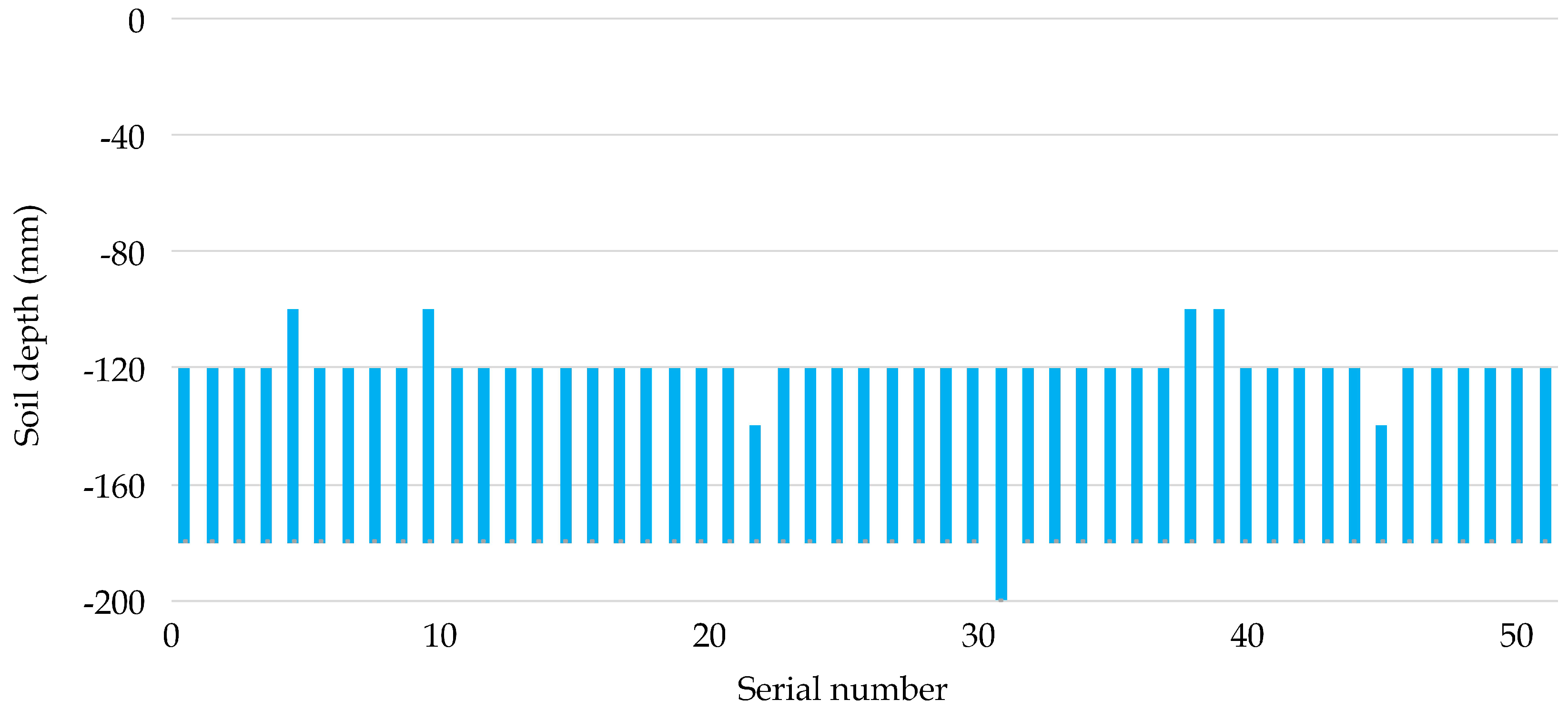
3.2. Fertilizer Depth

The minimum difference of the measurement results of the fertilizer distribution distance was 20 mm, because the field experiment used 20 mm as a layer to detect the fertilizer distribution. The distance between the upper and lower fertilizer openings of the opener was 100 mm, and the theoretical distribution distance of fertilizer in the vertical direction should be about 100 mm. As shown in Figure 10, it could be seen from the distribution distance of the fertilizer that the distribution distance in the soil was concentrated at 60 to 80 mm. When the distribution distance was 40 mm, it indicated that the accumulation of fertilizer was very serious, but it occupied less. The actual distribution distance of the fertilizer was lower than the theoretical distance, which was mainly because the backflow speed of the soil to the fertilizer ditch is lower than the falling speed of the fertilizer.
The actual distribution distance of the fertilizer in the field experiment was lower than the theoretical distance, mainly due to the downward movement of the fertilizer. This result corresponded to the overall downward movement of fertilizer in the simulation. A comparative analysis of the simulation and experimental results showed that both had the same motion law, which proved the accuracy of the simulation.

3.3. Comparison and Analysis of Simulation and Experiment Results

A comparison between the simulation results and the experiment results at different soil depths is shown in Figure 11 and Figure 12. The speed was the most important factor affecting the quality of fertilization. The result of the simulation and test at speeds of 1 and 1.6 m/s is shown in Figure 11 and Figure 12, respectively. It was difficult to detect fertilizer, and the method used in this paper was to layer the soil and detect the various sections. The fertilizer distribution and displacement at soil depths of 120, 140, 160, and 180 mm in the field experiment corresponded to the displacement of B-N-T-H, C-O-U-I, D-P-V-G, and E-Q-W-K among the four vertical edges of the simulation model. Table 5 shows the average displacement results of the simulation and the experiment in the horizontal and vertical directions at the speeds of 1 and 1.6 m/s, respectively.
To summarize, the trend and law of the simulation results based on the SPH simulation model were the same as the experiment results at different soil depths and working speeds. The simulation results of fertilizer displacement at different soil depths was close to the experiment results. Therefore, a model based on the SPH algorithm could be used to simulate and study the law of fertilizer movement in the soil and analyze the influence of key factors on the quality of fertilization.
The movement process of fertilizer in the soil under the action of the cover was very complicated. Due to the complexity of soil composition and the variability of soil parameters under the disturbance of working parts, it is very difficult to completely simulate the soil change. Therefore, the simulation is not as accurate as experiments in the real world and it is hard to simulate the movement process of fertilizer in the soil. We simulated the movement process of fertilizer to predict the variance trend and the law of fertilizer movement under the main influence factors and then compared the simulation results with the experiment results.
The simulation results of the model based on the SPH algorithm had the same variance trend as the experiment results, but there was still a difference between the simulation results and the experiment results. The simulation results were generally smaller than the experiment results. The reasons are as follows: (1) The simulation model was a simplification of the actual working parts. There is still a gap between the model parameters and the actual working condition; (2) This paper used a designed soil sampler to detect fertilizer distribution. Compared with the traditional cutting section method, this is a more reasonable and accurate detection method. The overall situation was represented by four sections, so it could not fully reflect the movement law and distribution of fertilizer; (3) In the experiment, the fertilizer was dropped into the soil, and the fertilizer had an initial velocity, which made the displacement larger, hence the simulation results were smaller than the experiment results.

4. Conclusions

In the present paper, the SPH method and a 3D model were used to simulate fertilizer movement and analyze influencing factors. The method and model were shown by a field experiment to be of generally good accuracy and effect in simulating the fertilizer movement process. By using the method and the model, the movement process and deformation of the fertilizer in three directions of X, Y, and Z under the action of a hill-drop fertilizer device were analyzed. According to the simulation results, the following observations were made: (1) Along the planter’s forward direction, the fertilizer displacement in the upper layer was larger, the fertilizer displacement in the lower layer was smaller, and the fertilizer displacement decreased from top to bottom; (2) In the vertical direction, the fertilizer overall moved downwards, and the falling displacement was close; (3) In the direction perpendicular to the planter’s forward direction, the fertilizer located on both sides of the opener moved toward the opener, and the displacement was small.
We then used the orthogonal simulation method to study the key factors affecting the overall deformation and displacement of the fertilizer, and used the range analysis method to analyze the simulation results of each index. The following conclusions were drawn: (1) The most important factors affecting the deformation coefficient in the vertical direction, the deformation coefficient in the forward direction, and the average point displacement were the forward speed of the planter, the cover depth, and the distance between the cover and the opener, respectively; (2) The optimal scheme was when the forward speed of the planter was 1.6 m/s, the cover depth was 100 mm, the distance between the cover and the opener was 140 mm, and the cover and the fertilizer pipe aligned from the center.
Validated by a field experiment, the results demonstrate the following: (1) As the soil depth increased, the offset distance of the fertilizer decreased; (2) The offset distance was large along the planter’s forward direction, and the offset distance perpendicular to the forward direction was small; (3) The distribution distance of the fertilizer was concentrated at 60 to 80 mm, which was lower than the theoretical distribution distance. Comparing the simulation results with the experiments, we concluded that although there were small differences between the fertilizer displacement calculated based on the SPH algorithm and the measuring results in the field experiment, they had the same variation trend. This means we can use this SPH method to analyze fertilizer movement law and influencing factors effectively.
In conclusion, our work demonstrates that there are merits to using the SPH method to analyze movement law and influencing factors. These merits are as follows: (1) The SPH method avoids the misconvergence caused by mesh distortion and increases the accuracy of the simulation; (2) The orthogonal simulation method considerably reduces the number of experimental groups under different working parameters and provides a theoretical foundation for optimizing working parameters; (3) This work proves that the factors that affect the movement of fertilizer in soil can be studied by simulation rather than by real experiments. This avoids the laborious experimental process and substantially reduces work time and cost.

Author Contributions

All authors contributed to the work. J.G. established the 3D model and performed the data analysis; J.Z. guided the research work and designed the experiment; J.G., Y.Z., and Z.H. performed the experiment; J.G. edited the paper; J.Z., F.Z., and L.G. proof-read the paper. All authors have read and agreed to the published version of the manuscript.

Funding

This research work is supported by the National Key Technology Research and Development Program of China (No. 2015BAD23B02).

Conflicts of Interest

The authors declare no conflict of interest.

References

  1. Oyebiyi, F.B.; Aula, L.; Omara, P.; Nambi, E.; Dhillon, J.S.; Raun, W.R. Grain yield response to methods of nitrogen fertilization. Commun. Soil Sci. Plant Anal. 2019, 50, 2694–2700. [Google Scholar] [CrossRef]
  2. Sweeney, D.W.; Ruiz-Diaz, D.; Jardine, D.J. Nitrogen management and uptake by corn on no-till and ridge-till claypan soil. Agrosyst. Geosci. Environ. 2018, 1. [Google Scholar] [CrossRef] [Green Version]
  3. Shiferaw, B.; Prasanna, B.M.; Hellin, J.; Bänziger, M. Crops that feed the world 6. Past successes and future challenges to the role played by maize in global food security. Food Secur. 2011, 3, 307–327. [Google Scholar] [CrossRef] [Green Version]
  4. Wu, N.; Lin, J.; Li, B. Design and test on no-tillage planter precise hole fertilization system. Trans. Chin. Soc. Agric. Machin. 2018, 49, 64–72. [Google Scholar]
  5. Liu, Z.; Wang, Q.; Liu, C.; Li, H.; He, J.; Liu, J. Design and experiment of precision hole-fertilizing apparatus with notched plate. Trans. Chin. Soc. Agric. Machin. 2018, 49, 137–144. [Google Scholar]
  6. Li, M.; Wen, X.; Zhou, F. Working parameters optimization and experiment of precision hole fertilization control mechanism for intertilled crop. Trans. Chin. Soc. Agric. Machin. 2016, 47, 37–43. [Google Scholar]
  7. Mouazen, A.M.; Nemenyi, M. Finite element analysis of subsoiler cutting in non-homogeneous sandy loam soil. Soil Tillage Res. 1999, 51, 1–15. [Google Scholar] [CrossRef]
  8. Shmulevich, I. State of the art modeling of soil–tillage interaction using discrete element method. Soil Tillage Res. 2010, 111, 41–53. [Google Scholar] [CrossRef]
  9. Ucgul, M.; Saunders, C.; Fielke, J.M. Discrete element modelling of tillage forces and soil movement of a one-third scale mouldboard plough. Biosyst. Eng. 2017, 155, 44–54. [Google Scholar] [CrossRef]
  10. Barr, J.B.; Ucgul, M.; Desbiolles, J.M.A.; Fielke, J.M. Simulating the effect of rake angle on narrow opener performance with the discrete element method. Biosyst. Eng. 2018, 171, 1–15. [Google Scholar] [CrossRef]
  11. Wang, Y.; Liang, Z.; Cui, T.; Zhang, D.; Qu, Z.; Yang, L. Design and experiment of layered fertilization device for corn. Trans. Chin. Soc. Agric. Machin. 2016, 47, 163–169. [Google Scholar]
  12. Gao, J.; Zhou, P.; Zhang, B.; Li, F. Development and test of high speed soil-cutting simulation system based on smooth particle hydrodynamics. Trans. Chin. Soc. Agric. Eng. 2007, 23, 20–26. [Google Scholar]
  13. Pastor, M.; Haddad, B.; Sorbino, G.; Cuomo, S.; Drempetic, V. A depth-integrated, coupled SPH model for flow-like landslides and related phenomena. Int. J. Numer. Anal. Methods Geomech. 2009, 33, 143–172. [Google Scholar] [CrossRef]
  14. Zhang, J.; Liu, H.; Gao, J.; Lin, Z.; Chen, Y. Simulation and test of corn layer alignment position hole fertilization seeder based on SPH. Trans. Chin. Soc. Agric. Machin. 2018, 49, 66–72. [Google Scholar]
  15. Ucgul, M.; Saunders, C.; Li, P.; Lee, S.-H.; Desbiolles, J.M.A. Analyzing the mixing performance of a rotary spader using digital image processing and discrete element modelling (DEM). Comput. Electron. Agric. 2018, 151, 1–10. [Google Scholar] [CrossRef]
  16. Bui, H.H.; Fukagawa, R.; Sako, K.; Ohno, S. Lagrangian meshfree particles method (SPH) for large deformation and failure flows of geomaterial using elastic-plastic soil constitutive model. Int. J. Numer. Anal. Methods Geomech. 2008, 32, 1535–1570. [Google Scholar] [CrossRef]
  17. Tran, H.T.; Wang, Y.N.; Nguyen, G.D.; Kodikara, J.; Sanchez, M.; Bui, H. Modelling 3D desiccation cracking in clayey soils using a size-dependent SPH computational approach. Comput. Geotech. 2019, 116, 17. [Google Scholar] [CrossRef]
  18. Ozbulut, M.; Yildiz, M.; Goren, O. A numerical investigation into the correction algorithms for SPH method in modeling violent free surface flows. Int. J. Mech. Sci. 2014, 79, 56–65. [Google Scholar] [CrossRef] [Green Version]
  19. Peng, C.; Xu, G.; Wu, W.; Yu, H.-S.; Wang, C. Multiphase SPH modeling of free surface flow in porous media with variable porosity. Comput. Geotech. 2017, 81, 239–248. [Google Scholar] [CrossRef]
  20. Zhang, A.; Sun, P.; Ming, F. An SPH modeling of bubble rising and coalescing in three dimensions. Comput. Methods Appl. Mech. Eng. 2015, 294, 189–209. [Google Scholar] [CrossRef]
  21. Bonet, J.; Kulasegaram, S.; Rodriguez-Paz, M.X.; Profit, M. Variational formulation for the smooth particle hydrodynamics (SPH) simulation of fluid and solid problems. Comput. Methods Appl. Mech. Eng. 2004, 193, 1245–1256. [Google Scholar] [CrossRef]
  22. Niu, W.; Mo, R.; Chang, Z.; Wan, N. Investigating the Effect of Cutting Parameters of Ti–6Al–4V on Surface Roughness Based on a SPH Cutting Model. Appl. Sci. 2019, 9, 654. [Google Scholar] [CrossRef] [Green Version]
  23. Gu, S.; Bo, F.; Luo, M.; Kazemi, E.; Zhang, Y.; Wei, J. SPH simulation of hydraulic jump on corrugated riverbeds. Appl. Sci. 2019, 9, 436. [Google Scholar] [CrossRef] [Green Version]
  24. Camporredondo, G.; Barber, R.; Legrand, M.; Muñoz, L. A Kinematic controller for liquid pouring between vessels modelled with smoothed particle hydrodynamics. Appl. Sci. 2019, 9, 5007. [Google Scholar] [CrossRef] [Green Version]
  25. Monaghan, J.J.; Lattanzio, J.C. A refined particle method for astrophysical problems. Astron. Astrophys. 1985, 149, 135–143. [Google Scholar]
  26. Liu, M.B.; Liu, G.R. Smoothed particle hydrodynamics (SPH): An overview and recent developments. Arch. Comput. Methods Eng. 2010, 17, 25–76. [Google Scholar] [CrossRef] [Green Version]
  27. Chen, X.; Wang, H. Slope failure of noncohesive media modelled with the combined finite–discrete element method. Appl. Sci. 2019, 9, 579. [Google Scholar] [CrossRef] [Green Version]
  28. Zheng, X.; Ma, Q.; Shao, S. Study on SPH viscosity term formulations. Appl. Sci. 2018, 8, 249. [Google Scholar] [CrossRef] [Green Version]
  29. Zheng, X.; You, Y.; Ma, Q.; Khayyer, A.; Shao, S. A comparative study on violent sloshing with complex baffles using the ISPH method. Appl. Sci. 2018, 8, 904. [Google Scholar] [CrossRef] [Green Version]
  30. Sakong, J.; Woo, S.C.; Kim, T.W. Determination of impact fragments from particle analysis via smoothed particle hydrodynamics and k-means clustering. Int. J. Impact Eng. 2019, 134, 15. [Google Scholar] [CrossRef]
  31. Hang, C.; Gao, X.; Yuan, M.; Huang, Y.; Zhu, R. Discrete element simulations and experiments of soil disturbance as affected by the tine spacing of subsoiler. Biosyst. Eng. 2018, 168, 73–82. [Google Scholar] [CrossRef]
  32. Li, P.; Ucgul, M.; Lee, S.-H.; Saunders, C. A new method to analyse the soil movement during tillage operations using a novel digital image processing algorithm. Comput. Electron. Agric. 2019, 156, 43–50. [Google Scholar] [CrossRef]
Figure 1. Corn hill-drop fertilizer planter.
Applsci 10 01643 g001
Figure 2. Movement process of the hill-drop fertilizer device, (a,d,g) at T = 0.35 s; (b,e,h) at T = 0.60 s; and (c,f,i) at T = 0.85 s.
Applsci 10 01643 g002
Figure 3. Fertilizer deformation schematic diagram: (a) fertilizer state before covering soil; (b) fertilizer state after covering soil.
Applsci 10 01643 g003
Figure 4. A–F movement process: (a) in the X direction; (b) in the Y direction; and (c) in the Z direction.
Applsci 10 01643 g004
Figure 5. M–R displacement results.
Applsci 10 01643 g005
Figure 6. Field performance experiment of corn hill-drop fertilizer planter.
Applsci 10 01643 g006
Figure 7. Flow chart showing the individual steps of the fertilizer extraction algorithm.
Applsci 10 01643 g007
Figure 8. Fertilizer distribution maps at different soil depths: (a) 120 mm; (b) 140 mm; (c) 160 mm; and (d) 180 mm.
Applsci 10 01643 g008
Figure 9. Fertilizer offset distances at different soil depths: (a) 120 mm; (b) 140 mm; (c) 160 mm; (d) and 180 mm.
Applsci 10 01643 g009
Figure 10. Fertilizer depth diagram of 50 groups.
Applsci 10 01643 g010
Figure 11. Comparison of simulation results and experiment results at different soil depths at 1 m/s.
Applsci 10 01643 g011
Figure 12. Comparison of simulation results and experiment results at different soil depths at 1.6 m/s.
Applsci 10 01643 g012
Table 1. Model parameter of soil particle and hill-drop fertilizer device.
TypeParameterValue
Soil particleBulk modulus (Mpa)5.9
Shear modulus (Mpa)2.7
Density kg m 3 1700
Moisture content (%)23.57
Specific gravity2.65
Angle of internal friction (rad)0.42
Cohesion (Kpa)12
Viscoplastic parameter1.1
Water density kg m 3 1000
Hill-drop fertilizer deviceDensity kg m 3 7850
Elastic modulus (Pa) 2.7 × 10 11
Possion’s ratio0.3
Table 2. Orthogonal factor level table of working condition parameters.
FactorV ( m s 1 ) B (mm)P (mm)L (mm)
Level11.05050110
21.30100140
31.6−50150170
Table 3. Simulation results of index ε .
NumberV ( m s 1 ) B (mm)P (mm)L (mm)Value
111110.021
212220.061
313330.069
421230.082
522310.024
623120.028
731320.038
832130.002
933210.001
K 1 0.1510.1410.0510.046Influence order: V, L, P, B
K 2 0.1340.0870.1440.127
K 3 0.0410.0980.1310.153
R0.1100.0540.0930.107
Optimal scheme V 3 B 2 P 1 L 1
Table 4. Simulation results of index λ .
NumberV ( m s 1 ) B (mm)P (mm)L (mm)Value
111110.062
212220.005
313330.102
421230.032
522310.021
623120.022
731320.060
832130.025
933210.021
K 1 0.1690.1540.1090.104Influence order: P, B, V, L
K 2 0.0750.0510.0580.087
K 3 0.1060.1450.1830.159
R0.0940.1030.1250.072
Optimal scheme V 2 B 2 P 2 L 2
Table 5. Simulation results of index S.
NumberV ( m s 1 ) B (mm)P (mm)L (mm)Value
111115.32
212227.07
313339.52
4212315.96
522319.72
623126.11
731327.09
832136.71
933216.31
K 1 21.9128.3718.1421.35Influence order: L, V, P, B
K 2 31.7923.5029.3420.27
K 3 20.1121.9426.3332.19
R11.684.4311.2011.92
Optimal scheme V 3 B 3 P 1 L 2

