A Novel Self-Healing Strategy for Distribution Network with Distributed Generators Considering Uncertain Power-Quality Constraints

Abstract

Self-healing of smart distribution networks with distributed generators, which are usually operated as independent islands after fault, can improve power-supply reliability. As a hot research topic, a self-healing scheme is usually treated as the output of a nonlinear optimizuoation model. However, existing strategies have two main shortcomings. The first, high-optimization dimension, results in low-optimization efficiency. The second, the effects of power-quality issues, which are more serious on islands and may further threaten the safe operation of islands, is usually neglected. To quickly obtain a reliable self-healing scheme, a novel strategy is proposed. As the first step, the distribution network after a fault occurrence can be divided into several trouble-free subnets via the connectivity analysis; each subnet is called an initial island. Further, for each initial island, a two-step optimization model of self-healing, which consists of load-shedding optimization and network reconfiguration optimization, is proposed to obtain the self-healing strategy with lower searching space as well as higher solving efficiency. In detail, in load-shedding optimization, by means of heuristic differential evolution algorithm, larger total recovery capacity is achieved by considering the droop characteristic of distributed generators (DGs) within the permissible change in frequency. In network-reconfiguration optimization, based on the improved hybrid particle swarm optimization algorithm, a comprehensive set of power-quality constraints, including constraint of change in frequency, uncertain constraints of node voltage total harmonic distortion (THD), and negative sequence components of DGs, is developed to guarantee the reliability of each island. To evaluate whether the constraints are satisfied during the optimization procedure, an improved flexible power-flow algorithm is developed to calculate the power flow of each island under change in frequency. Further, 2m+1-point estimate method is employed for uncertainty analyses of the distributions of harmonic and negative sequence components caused by the uncertainty of corresponding sources. Finally, via a 94-node practical distribution network, the effectiveness and advantages of the proposed strategy in safety, recovery capacity, and optimization efficiency are verified.

1. Introduction

As a core feature of smart distribution network (SDN), fast power-supply restoration after faults, which can reduce the adverse impacts of outage and abrupt faults, has important implications for both energy-supply companies and consumers. In recent years, technological advances and wide applications of distributed generators (DGs) provided powerful technical support for self-healing recovery of SDN.

The self-healing of SDN with DGs supported is generally treated as a nonlinear combinatorial optimization model with multiple objects and multiple constraints [1,2,3,4,5,6,7,8,9]. Existing researches mainly focus on the following issues.

(1) Total capacity of recovered loads [1,2,3,4,5,6,7,8,9]: As the basic goal of self-healing recovery, de-energized loads must be restored as quickly as possible.

(2) Load/consumer priority [2,3,4,5,6,9]: In actual distribution networks, priority of different loads is distinguished and the loads/consumers of higher priority shall be recovered preferentially.

(3) Number of switching operations [6,7,9]: As switching operations are time consuming and have operational cost, the number of switching operations shall be minimized to realize faster recovery and lower cost.

(4) Power loss [8,9]: For economical operation, the smaller the power loss of a self-healing scheme, the better.

Good results have been achieved in References [1,2,3,4,5,6,7,8,9]. However, existing strategies have two main shortcomings. The first, high-optimization dimension, results in low-optimization efficiency. The second, the effects of power quality issues, which are more serious in islanding and may further threaten the safe operation of islands, are usually neglected.

With wide application of power electronic devices and access to various nonlinear loads, a series of power-quality issues, such as harmonic pollution and negative sequence component injection, widely exist. As the capacity of each operating island is smaller compared with normally operated SDN, these issues will be more serious and may affect the safe operation of islands. For synchronous generator-based DG, serious negative sequence currents may result in being out of service [10,11]. For inverter-interfaced DG (IIDG), serious harmonic or negative sequence components may result in output oscillation or even in becoming out of service [12,13,14]. Serious harmonic component can lead to misoperation or could even cause harmonic sensitive load and equipment to stop working [15,16]. Therefore, power-quality issues may result in power unbalance of island and further lead to recovery failure. Thus, to prevent potential recovery failures caused by power-quality issues, it is necessary to uniformly consider the influences of harmonic and negative sequence components in the analysis of self-healing of SDN. Furthermore, as the injections of harmonic and negative sequence sources are uncertain and fluctuant, it is necessary to employ the uncertainty analysis method to obtain an optimal self-healing scheme in accordance with the distribution network actual operation.

In this paper, to realize faster, stronger, and safer recovery, a new self-healing recovery strategy is proposed. To improve optimization efficiency, a decoupled two-step optimization model of load-shedding and network-reconfiguration is established. To enlarge recovery capacity, the droop characteristic of DGs is considered in load-shedding within the permissible change in frequency. To prevent potential recovery failure caused by power-quality issues, a comprehensive set of power-quality restraints, including frequency constraint, uncertain constraints of harmonic, and negative sequence components, is established in the network reconfiguration optimization model.

This paper is organized as follows: Section 2 puts forward the framework of the proposed self-healing recovery strategy. Detailed instructions of the load-shedding optimization model are illustrated in Section 3. The network reconfiguration optimization model, considering uncertain power quality constraints, is minutely explained in Section 4. In Section 5, the solved algorithms of the proposed strategy are illustrated. Effectiveness and superiorities of the proposed strategy are further verified in Section 6. Finally, conclusions are drawn in Section 7.

2. Framework of the Proposed Self-Healing Recovery Strategy

In this section, the framework of the self-healing recovery strategy proposed in this paper, which is as shown in Figure 1, is illustrated.

Once a fault of SDN is detected by distribution automation system (DAS), the self-healing recovery strategy is put forward as follows.

(1) The distribution network after a fault occurrence can be divided into several trouble-free subnets, each of which is called an initial island. At the first step, the initial island division is carried out based on the connectivity analysis of the distribution network and each initial island is the minimum application object of optimization model of self-healing, which consists of load-shedding optimization and network reconfiguration optimization; the following two points are important for island division.

✓

Keep the normal operation of widely distributed high-priority loads as normal as possible.

✓

The island with larger capacity and more adjustable equipment can achieve better power quality indexes.

Based on the above understandings, the following initial island division strategy is adopted with the consideration of tie-switches.

(a)

If the network is connected after the fault, the network is operated as a whole island.

(b)

If the network is no longer connected after the fault but the connectivity can be recovered by the tie-switches, the network is still operated as a whole island.

(c)

If the network is no longer connected after the fault and the connectivity cannot be recovered by the tie-switches, the network shall be divided into independent small islands.

In the proposed strategy, the method in Reference [17] is used to judge the network connectivity.

The algorithm to judge the network connectivity is explained as follows.

(a) G = (A, E) is a network diagram, A = (A₁, A₂, …, A_n) is a set of the nodes, and E is a set of the lines.

(b) Z is an adjacency matrix, Z[i, j] = 1 if (A_i, A_j)∈E; otherwise, Z[i, j] = 0.

(c) Referring to the short connection in the circuit, the network diagram can be simplified in a similar way. If two nodes are directly connected, they can be merged into one node to form a new network graph.

For example, if node i is connected to node j, which means Z[i,j] = 1, the simplification of the network diagram can be operated as follows. In detail, for a row operation, apply the “OR” operation to the corresponding element of row i and row j, and the result is placed in row j. For a column operation, apply the “OR” operation to the corresponding element of column i and column j, and the result can be placed in column j. After the operations, the diagonal element can be set to zero. Since node i has been merged into node j, row i and column i are removed. The above simplification decreases the dimension of adjacency matrix Z from n to n-1.

(d) Repeat the simplification. The network diagram is not connected if there is a row in which all the elements are zeros during the process. Otherwise, the network diagram is connected, and when the dimension decreases to 2, all nondiagonal elements of adjacency matrix Z are 1.

Through the above simplification, each connected part of the network diagram is considered as an initial island.

After the initial island division, the proposed load-shedding optimization and network reconstruction optimization are applied for each initial island. In practical application, this procedure is in parallel for each island, thus the increase of the number of initial islands may lead to the growth of the total amount of computational burden, but it will not lead to the delay of strategy implementation for each initial island by taking advantage of parallel computation. In consequence, there is no specific restrictions on the number of islands.

(2) For each initial island, the load-shedding optimization and network reconfiguration optimization are carried out as follows, respectively.

(a)

In the load-shedding optimization model, on one hand, the droop characteristic of DGs is considered to enlarge the sum recovery capacity within the allowable change in frequency. On the other hand, load priority is introduced to guarantee the normal operation of the loads that are more important. Concrete illustrations of the load-shedding optimization model are proposed in Section 3.

(b)

In the network reconfiguration optimization model, the comprehensive set of power-quality constraints is considered so the obtained recovery scheme of the island can achieve good power-quality indexes. By this way, the threats caused by power-quality issues, such as high node voltage total harmonic distortion and excessive negative sequence current, can be prevented to guarantee the safe operation of the obtained island. Concrete illustrations of the load-shedding optimization model are proposed in Section 4.

3. Load-Shedding Optimization Model

3.1. Optimization Variables

In the load-shedding optimization model, the variables are the shedding state of each load, which is treated as 0–1 type variable. Concretely, x_ik = 1 means that the load of node i on the kth island is shed, while x_ik = 0 means the load is maintained.

3.2. Objective Function

In this section, the aim is to minimize the sum capacity of shed loads with the consideration of load priority. Thus, the objective function of load-shedding is as follows.

$$L_{s\_k}=min{\displaystyle \sum _{i=1}^m{x}_{ik}{P}_{Li}{\lambda }_i}$$

(1)

where L_s, m, k, P_Li, and λ_i are the minimum of load-shedding of all the nodes, the total number of loads, the number of the island to be studied, active power, and weighting coefficient of the load of node i on island k, respectively.

In detail, λ_i is set as follows in this paper according to a lot of tests.

(1) For important loads (L2), λ_i = 100.

(2) For sub-important loads (L1), λ_i = 10.

(3) For general loads (L0), λ_i = 1.

3.3. Constraints

(1) Active power balance constraint considering the droop characteristic of DGs.

The active power shortage is supposed to be smaller than the result of DGs’ generated active power minus P_Los0.

$$P_{Lto\_re}={\displaystyle \sum _{i=1}^m(1-x_{ik})}{P}_{Li}\le {\displaystyle \sum _{j=1}^{n_k}{P}_{DGj\_f}-P_{Los0}}$$

(2)

where P_{Lto_re} represents the total active power capacity of the recovered loads, P_{Los_0} is the initial active power loss of the initial island to be studied, and P_{DGj_f} is the output active power of jth DG under frequency f if the DG can participate frequency modulation, which can be calculated according to the droop characteristic as follows [18].

$$P_{DGj\_f}=P_{DGj\_r}\times [1+K_{pfj}(f_r-f)/f_r]$$

(3)

where P_{DGj_r} is the rated output active power of jth DG under rated frequency f_r and K_pfj is its active power-frequency adjustment coefficient. According to Reference [19], f_r and the minimum value of f are set as 50 Hz and 49.5 Hz, respectively.

Thus, to maximize the total recovery capacity, P_{DGj_max}, which is the maximum value of P_{DGj_f}, can be calculated by setting the value of f as 49.5 Hz as follows.

$$P_{DGj\_\mathit{max}}=P_{DGj\_r}\times [1+K_{pfj}(50-49.5)/50]$$

Correspondingly, Equation (2) can be modified as the equation below.

$$P_{Lto\_re}={\displaystyle \sum _{i=1}^m(1-x_{ik})}{P}_{Li}\le {\displaystyle \sum _{j=1}^n{P}_{DGj\_\mathit{max}}-P_{Los0}}$$

(2) Reactive power balance constraint

The reactive power shortage is supposed to be smaller than the result of DGs’ generated reactive power plus Q_cmax.

$${\displaystyle \sum _{i=1}^m(1-x_{ik})Q_{Li}\le {\displaystyle \sum _{j=1}^n{Q}_{DGj\_\mathit{max}}+Q_{c\mathit{max}}}}$$

(4)

where x_ik is defined in Section 3.1, Q_Li is the reactive power of the ith load, and Q_cmax represents the maximum total reactive compensation capacity of the initial island. Q_{DGj_max} is the maximum allowable reactive power of the jth DG, which is decided by the apparent power constraint as follow:

$$Q_{DGj\_\mathit{max}}=\sqrt{{(S_{DGj\_\mathit{max}})}^2-{(P_{DGj\_\mathit{max}})}^2}$$

where S_{DGj_max} and P_{DGj_max} are the maximum apparent power and active power of the jth DG.

4. Network-Reconfiguration Optimization Model

As the second step, network reconfiguration is based on the optimal load-shedding scheme obtained in Section 3.

4.1. Optimization Variables

In network-reconfiguration optimization, the state of each switch and the specific compensation capacity of each reactive power compensation device are treated as 0–1-type and integer-type variables, respectively.

4.2. Objective Function

Considering rapidity, reliability, and economy, network-reconfiguration optimization aims at minimizing the number of switching operations. Concrete objective function can be expressed as follows:

$$min(F(s,t)={\displaystyle \sum _{a=1}^{k_1}abs(s_a-s_{a\_ini})}+ {\displaystyle \sum _{b=1}^{k_2}abs(t_b-t_{b\_ini})}$$

(5)

where k₁ and k₂ are the amount of section switches and tie-switches of the island, respectively; s_a and s_{a_ini} are the optimized and initial states of the ath section switch, respectively; and t_b and t_{b_ini} are the optimized and initial states of the bth tie-switch.

4.3. Constraints of Network-Reconfiguration

(1) Regular constraints

(a) DG apparent power constraint.

$$S_{DGj}\le S_{DGj\_\mathit{max}}$$

(6)

where S_DGj is the apparent power of the jth DG.

(b) Branch distribution power constraint.

$$S_c\le S_{c\_\mathit{max}}$$

(7)

where S_{c_max} is the maximum allowable value of S_c, which is the distribution power of the cth branch.

(c) Node voltage amplitude constraint.

$$V_{i\_\mathit{min}}\le V_i\le V_{i\_\mathit{max}}$$

(8)

where V_{i_min} and V_{i_max} represent the lower and upper limits of V_i, which is the voltage amplitude of node i.

(2) Comprehensive power quality constraints set

$$\{\begin{array}{l}THD-u{l}_i \le TH{D}_{\mathit{max}}\\ Cune-u{l}_j\le C{u}_{\mathit{max}}\\ Vone-u{l}_k\le V{o}_{\mathit{max}}\\ \Delta f\le \Delta f_{max}\end{array}$$

(9)

(a) Uncertain node voltage total harmonic distortion (THD) constraint.

$$THD-u{l}_i \le TH{D}_{\mathit{max}}$$

(10)

where THD-ul_i is the upper limit of the distribution range of the THD index of node i. THD_max is the permissible maximum value of THD, which is defined as 4% for the distribution network of 10 kV according to Reference [20].

(b) Uncertain negative sequence current constraint for synchronous generator-based DG

$$Cune-u{l}_j\le C{u}_{\mathit{max}}$$

(11)

where

$$Cune-u{l}_j=Ine{-\mathit{ul}}_j/I{n}_j$$

where Ine-ul_j is the upper bound of distribution range of the actual negative sequence current of the jth synchronous generator-based DG while In_j is the rated positive sequence current. Cu_max is the permissible maximum value, which is set as 10% referring to Reference [21].

(c) Uncertain negative sequence voltage constraint for IIDG

$$Vone-u{l}_k\le V{o}_{\mathit{max}}$$

(12)

where

$$Vone-u{l}_k=Vne{-\mathit{ul}}_k/V_k$$

where Vone-ul_j is the upper bound of the distribution range of the actual negative sequence voltage of the kth IIDG while V_k is the actual positive sequence voltage of the kth IIDG. Vo_max is the permissible maximum value, which is set as 2% referring to Reference [22].

(d) Constraint of island’s change in frequency

$$\Delta f\le \Delta f_{max}$$

(13)

where

$$\Delta f=abs(f_r-f)$$

According to Reference [19], Δf_max, which is the maximum allowable value of change in frequency Δf, is 0.5 Hz.

5. Solving Algorithms

In this paper, the heuristic differential evolution algorithm and improved hybrid particle swarm optimization algorithm [23] are used to seek the optimal load-shedding scheme and network-reconfiguration scheme, respectively. The optimal solutions of the two models constitute the whole recovery scheme.

To evaluate whether the constraints are satisfied during the optimization procedure, an improved flexible power-flow algorithm for distribution network including second-order items is developed to calculate the power flow of each island under change in frequency. Also, 2m+1 point estimate methods (PEM), which has higher computational efficiency while the accuracy is almost the same as the Monte Carlo method, is chosen to carry out uncertainty analysis.

Detailed illustrations of the two algorithms are as follows.

5.1. Improved Flexible Power-Flow Algorithm for Distribution Network including Second-Order Items

In Reference [24], in order to obtain the generic initial value of the distribution network power flow, the equations are transformed to quadratic matrix equations in which the second-order items and droop characteristic of DGs and load are considered. It is expressed as the following equation.

$$J\Delta x+\stackrel{\sim }{\Delta x}J\Delta x=S_L$$

(14)

In the equation

$$J=\left[\begin{array}{cc}-G& B\\ B& G\end{array}\right],S_L=\left[\begin{array}{c}p\\ q\end{array}\right],\stackrel{\sim }{\Delta x}=\left[\begin{array}{cc}\stackrel{\sim }{\Delta e}& -\stackrel{\sim }{\Delta f}\\ \stackrel{\sim }{\Delta f}& \stackrel{\sim }{\Delta e}\end{array}\right],\stackrel{\sim }{\Delta e}=diag(\Delta e_i),\stackrel{\sim }{\Delta f}=diag(\Delta f_i)$$

B is the imaginary component of the network node admittance matrix and G is the real component.

Concrete derivations and statements of the above equation can be found in Reference [24]. For Equation (14), its solving efficiency is restricted by the fsolve function of MATLAB.

To overcome the shortage, the solution issue of Equation (14) is proposed to be converted into a nonlinear constrained optimization problem and solved via the sequential quadratic programming (SQP) method in this paper.

Actually, Equation (14) contains 2n equations. If one moves S_L to the left side of the equation, Equation (14) can be written as follows.

$$\begin{array}{l}\Delta x^T{a}_i\Delta x+b_i{}^T\Delta x-p_{Li}=0,i\in (1,n)\\ \Delta x^T{c}_i\Delta x+d_i{}^T\Delta x-q_{Li}=0,i\in (1,n)\end{array}$$

(15)

Generally, Equation (15) can be written as the uniform expression below.

$$\Delta x^T{r}_i\Delta x+s_i{}^T\Delta x-t_i=0,i\in (1,2n)$$

(16)

Then, Equation (16) can be transformed into the following nonlinear constrained optimization model.

$$\begin{array}{l} min(abs(\Delta x^T{r}_k\Delta x+s_k{}^T\Delta x-t_k)) k\in (1,2n)\\ s.t. \Delta x^T{r}_i\Delta x+s_i{}^T\Delta x-t_i=0,i\in (1,2n)\&i\ne k\end{array}$$

(17)

As SQP has the characteristics of good global convergence as well as excellent local super-linear convergence [25]; better performances of convergence and computing efficiency can be achieved by the improved solving method.

5.2. 2m+1 Point Estimate Method

The 2m+1 PEM, in which m represents the number of input random variables, can be used to calculate the statistical moments of a random quantity, which is a function of one or several random variables [26]. Compared with the two-point estimate method, the accuracy of 2m+1 PEM is higher. To get the statistical moments of output random variables, the function has to be calculated 2m+1 times [27].

Let X_i denote a random variable and Y = f(X₁, X₂, …, X_i) be the function of X_i. The procedures for finding the moments of the output Y by 2m+1 PEM are as follows.

(1) Find probability concentrations of each input random variable.

$$x_{i,k}={\mu }_i+{\theta }_{i,k}{\sigma }_i (k=1,2)$$

(18)

where x_i,k is the concentration of X_i; μ_i and σ_i are the mean and standard deviation of X_i; and θ_i,k is the location-factor, which can be obtained as follow:

$${\theta }_{i,k}=\frac{{\alpha }_{i,3}}{2}+{(-1)}^{3-i}\sqrt{{\alpha }_{i,4}-\frac{3}{4}{\alpha }_{{}_{i,3}}^2} k=1,2$$

(19)

where α_i,r is the rth standardized central moment of X_i and can be obtained by the following Equation.

$${\alpha }_{i,r}=\frac{{\lambda }_{i,r}}{{\sigma }_i^r}=\frac{E[{(X_i-{\mu }_i)}^r]}{{\sigma }_i^r} r=3,4$$

(20)

where E[(x_i−μ_i)^r] is the rth central moment of X_i.

(2) Determine the 2m+1 estimation points.

According to Equations (17)–(19), each random variable can be estimated by 2 points; the 2m estimation points can be determined as follows:

$$({\mu }_1,{\mu }_2,\dots ,x_{i,k}\dots ,{\mu }_m) k=1,2 i=1,2,\cdots ,m$$

(21)

The special addition of the 2m estimation points is the point of x_μ, which is constituted by the means of all the input random variables:

$$x_{\mu }=({\mu }_1,{\mu }_2,\cdots ,{\mu }_i,\cdots {\mu }_m)$$

(22)

(3) According to Equations (19)–(20), the weighting factors are as follows:

$$\{\begin{array}{l}{p}_{i,k}=\frac{{(-1)}^{3-k}}{{\theta }_{i,k}({\theta }_{i,1}-{\theta }_{i,2})} k=1,2\\ p_{\mu }=1-{\displaystyle \sum _{i=1}^m\frac{1}{({\alpha }_{i,4}-{\alpha }_{{}_{i,3}}^2)}}\end{array}$$

(23)

${\displaystyle \sum _{i=1}^m}{\displaystyle \sum _{k=1}^2}{p}_{i,k}+p_{\mu }=1,{\displaystyle \sum _{k=1}^2}{p}_{i,k}=\frac{1-p_{\mu }}{m}$, respectively.

(4) According to Equations (21)–(23), calculate the jth moment of Y.

$$E(Y^j)\approx {\displaystyle \sum _{k=1}^2{\displaystyle \sum _{i=1}^m\{p_{i,k}}}{[f({\mu }_1,{\mu }_2,\dots ,x_{i,k}\dots ,{\mu }_m)]}^j\}+p_u{[f(x_{\mu })]}^j$$

(24)

(5) Compute the mean value and standard deviation of Y.

$$\{\begin{array}{l}u(Y)=E(Y)\\ \sigma (Y)=\sqrt{E(Y^2)-{(E(Y))}^2}\end{array}$$

(25)

5.3. Uncertainty Analyses of Harmonic and Negative Sequence Components Based on the 2m+1 PEM

The load-shedding optimization model and network reconfiguration optimization model make strategies according to the current electrical quantity and network topology collected by the distribution network automation system. According to the description in chapter 2 of the original manuscript, this information is deterministic; thus, the optimization models also adopt deterministic models and power-flow algorithm for the fundamental component.

In the network reconfiguration model, power-quality indexes are required to meet the constraints not only at the current moment but also in the following period of time. This is also one of the main contributions of this paper. In the following period of time, the power-quality index is uncertain, so the harmonic power flow and the unbalanced power flow of the fundamental component are obtained based on the 2m+1 PEM method, in which the estimation accuracy is similar to the classical Monte Carlo method but computational burden is much less to accommodate the need for online application.

In this paper, uncertainty analyses of harmonic and negative sequence components are independent of each other. The harmonic power-flow calculation adopts the method used in References [10,28,29]. The negative sequence component calculation method used in References [30,31,32] is introduced to analyze the ranges of system’s negative sequence currents.

Due to the similarity of the two analyses, harmonic uncertainty analysis is chosen as the example to give detailed descriptions. Specific steps are as follows.

(1) The sequences of the measured harmonic current values of harmonic sources are presented to calculate the mean and variance of each variable.

(2) Calculate the 2m+1 estimation points and corresponding weighting factors via Equations (21)–(23).

(3) Carry out harmonic power-flow calculation 2m+1 times to obtain all the results of f(μ₁, μ₂, …, μ_i) and f(x_μ).

(4) Multiply the results of step 3 and their corresponding weighting factors together to get the expectation μ(Y_k) and standard deviation σ(Y_k) of each output variable Y_k according to Equations (24) and (25).

(5) Obtain the distribution range of Y_k as $[\mu (Y_k)-2\sigma (Y_k), \mu (Y_k)+2\sigma (Y_k)]$.

The reasons to select $[\mu (Y_k)-2\sigma (Y_k), \mu (Y_k)+2\sigma (Y_k)]$ as the distribution range of $Y_k$ are as follows.

✓

For normal distributions, the probability of the observed value within $[\mu (Y_k)-2\sigma (Y_k), \mu (Y_k)+2\sigma (Y_k)]$ is about 95.45%.

✓

The event with probability less than 5% generally can be treated as a small probability event.

If Y_k is node voltage total harmonic distortion, negative sequence current of synchronous generator-based DG, and negative sequence voltage of IIDG, the upper bound $\mu (Y_k)+2\sigma (Y_k)$ will be THD-ul, Cune-ul, and Vone-ul, respectively.

6. Cases Studies

6.1. Introductions of a Practical Complex Distribution Network and Scenarios

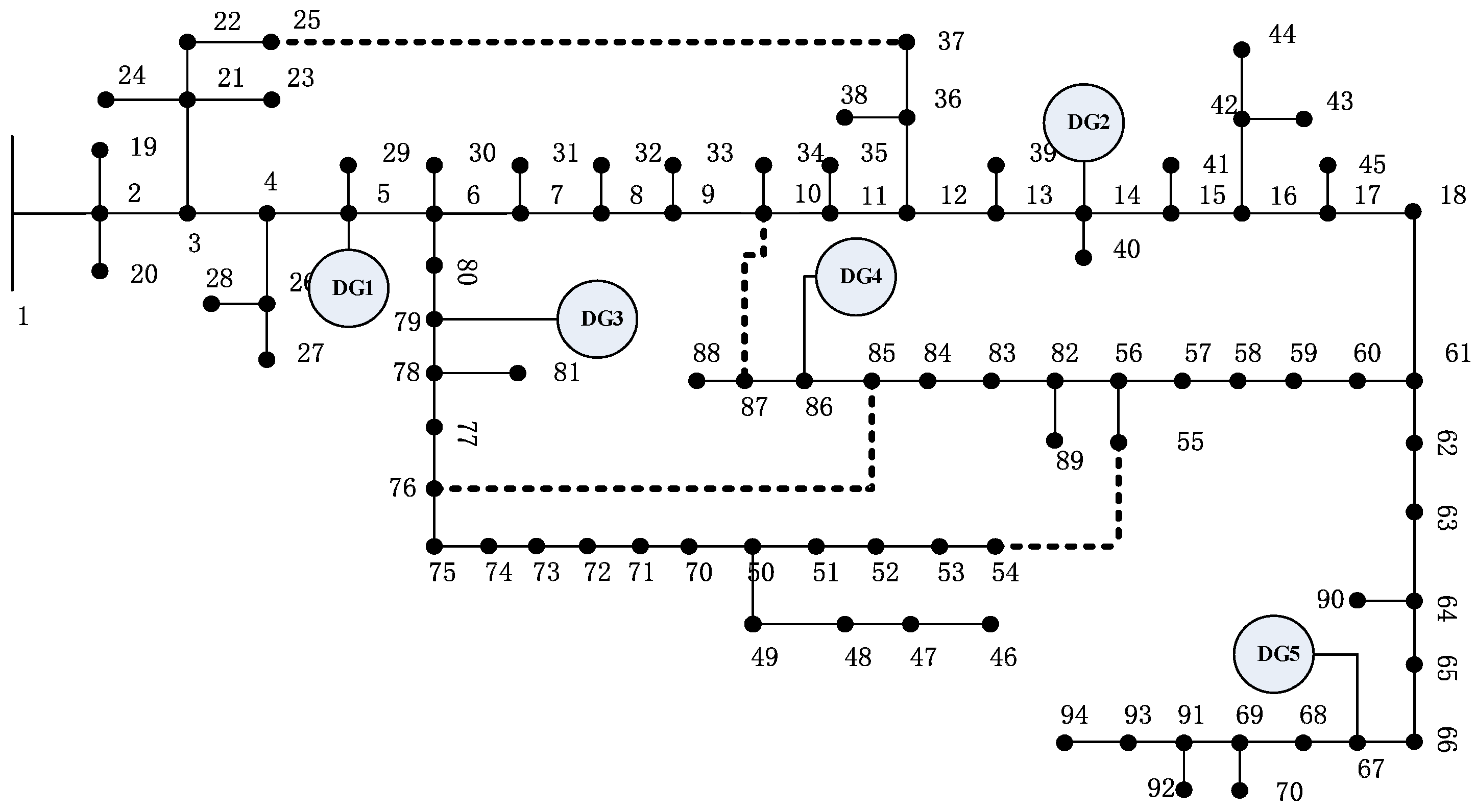
To fully demonstrate the effectiveness and advantages of the proposed strategy, lots of tests verified by simulations via ETAP power system simulation software have been done via several examples with different operation status. Due to limited space, a practical complex distribution network in China, which is shown as Figure 2, is used to give detailed descriptions.

The practical complex distribution network contains 94 nodes, 93 branches, 4 tie lines (10–87, 25–37, 54–55, and 76–85), and 5 DGs. In the case of normal power supply, total capacity of all the loads is 13,379.29 kW + 4519.12 kvar. Two reactive power compensations are installed on node 11 and node 59, respectively. A fluctuant harmonic source and a negative sequence current source, which fit normal distribution, are set at node 51 and node 61, respectively. Limited by space, more detailed instructions of the distribution network are listed in

Table A1. Concrete parameters of the 5 DGs.

	Rated Active Power/MW	Rated Power Factor	Kpfj	Reserve Capacity
DG1	0.4	0.8	20	20%
DG2	0.5	1	0	0%
DG3	0.8	1	0	0%
DG4	1.5	0.8	20	20%
DG5	1.5	0.8	20	20%

and

Table A2. Load priority.

Load Priority	Node	Total Active Power/MW	Total Reactive Power/MW
general	20, 24, 25, 28, 30, 31, 32, 34, 35, 38, 41, 43, 45, 47, 48, 52, 53, 54, 58, 60, 62, 66, 70, 71, 73, 74, 75, 76, 77, 80, 81, 82, 84, 85, 87, 89, 90, 94	9.34694	3.15796
Sub-important	19, 29, 39, 44, 49, 55, 57, 59, 63, 65, 72, 83, 86, 88, 92, 93	3.65392	1.23401
Important	33, 37, 40, 51, 61, 68	0.37843	0.12715

of Appendix A.

For the distribution network, the following benchmark scenario is selected as the typical situation to give detailed descriptions:

Benchmark scenario: disconnected with network and DG1, DG2, and DG3 are out of the running.

It is worth mentioning that the methods proposed in this paper can be applied to the distribution network benchmarks with different scales and topologies as well as to different scenarios of the same benchmarks under electrical faults at different locations.

6.2. Initial Results of Island Division

Based on the island division strategy proposed in Section 1, under the above scenario, the distribution network can be divided into islands.

For the benchmark scenario, the connectivity of the test system is not changed; therefore, the distribution network does not need to be divided into multiple islands.

6.3. Comparisons of the Proposed Strategy and the Conventional Strategy

To illustrate the superiorities of the proposed self-healing strategy, the benchmark scenario is studied to provide detailed comparison. Scheme 1 is the self-healing scheme obtained by the proposed strategy. Scheme 2 is the self-healing scheme obtained by the conventional strategy, in which the power quality constraint set and droop characteristic of DGs are not considered. The values of power-quality indexes of Scheme 2 are calculated. Concretely, the two schemes are minutely listed in the following

Table 1. Result of Scheme 1 and Scheme 2 for benchmark scenario.

		Scheme 1	Scheme 2
Total load removal/kw		9830.21	10,429.43
Normal loads		All cut	All cut
Sub-important loads		Cut 39, 72, 83	Cut 19, 44, 49, 57, 72, 86
Important loads		All recovered	All recovered
Number of switch actions		2 times, 8–9 open, 10–87 close	0
Frequency/Hz		49.5273	50.02
Reactive compensation/kvar	Node 11	190	240
	Node 59	0	125
Vone-ul/%	DG4	1.47	1.44
Cune-ul/%	DG5	9.80	10.56
THD-ul/%	min	3.34	4.41
	max	3.42	4.54

.

From Table 1, the following advantages of the proposed strategy can be summarized.

(1) Total recovery capacity is larger. Specifically, total load removal of Scheme 1 is 9830.21 kW, while the value of Scheme 2 is 10,429.45 kW. That is, the total recovery capacity has risen nearly 20.31% from 2949.84 kW to 3549.08 kW, which means the proposed strategy can realize stronger recovery.

(2) The obtained recovery scheme has better power- quality indexes and higher reliability.

✓

On one hand, the Cune-ul index of DG5 in Scheme 2 exceeds the negative sequence protection action threshold value of 10%. It may cause DG5 to quit operation and may further result in operation failure of the recovered island as power imbalance.

✓

On the other hand, THD-ul indexes of all nodes in Scheme 1 are less than 4% as the maximum is 3.42%, while THD-ul indexes of all nodes in Scheme 2 are exceeded as the minimum is 4.41%. The excessive THD may cause abnormal operation or may cause the equipment to quit working. That is, the reliability of Scheme 2 will not be guarantee.

To sum up, the proposed strategy can realize the larger total recovery capacity and higher reliability by considering the DG frequency adjustment characteristic and the comprehensive set of power-quality constraints.

6.4. Necessity of Harmonic and Negative Uncertainty Analyses

To illustrate the necessity of uncertainty analysis, Scheme 2 is further analyzed by contrasting the THD-ul and THD-me indexes and the Cune-ul and Cune-me indexes which are minutely listed in

Table 2. Comparison of THD-ul and THD-me for Scheme 2.

	THD-ul	THD-me
minimum	4.41%	3.59%
maximum	4.54%	3.70%

and

Table 3. Comparison of Cune-ul and Cune-me for Scheme 2.

	Cune-ul	Cune-me
DG5	10.56%	8.72%

, respectively. THD-me and Cune-me are the midpoints of the distribution ranges of THD index and negative sequence current, respectively.

Through the above two tables, it can be illustrated that the values of THD-me and Cu-me are more conservative. Thus, recovery failure may be caused, as the scheme with actually exceeded power-quality indexes is treated as a feasible scheme. Reasons are as follows.

(1) As all the nodes in THD-me are smaller than 4%, Scheme 2 is a feasible scheme in the view of THD-me. However, meanwhile, the values of THD-ul index of all the nodes are within (4.41%, 4.54%) which are larger than 4%.

(2) Cune-me index of DG5 is within 10%, so Scheme 2 can be treated as a feasible one from the perspective of Cune-me. However, the Cune-ul index of DG5 is clearly exceeded.

Thus, in accordance with operation practices of power grids, it is necessary to adopt the uncertainty analysis method to deal with the uncertainty of harmonic and negative sequence components.

6.5. Solution Efficiency Comparison

Moreover, a comparison is conducted to illustrate the advantage of the proposed two-step optimization model. The computing platform is a PC with Intel i7-4790@3.60GHZ CPU and 8G RAM (Intel, Santa Clara, CA, USA), and the software environment is Windows 10 Professional and MATLAB R2010b (MathWorks, Natick, MA, USA).

Concretely, the proposed two-step optimization model and the conventional one-layer optimization model are used to find the recovery for benchmark scenario. Specific information of the two recovery schemes is shown in

Table 4. Results of the two-step optimization model and the single-layer optimization model for benchmark scenario.

		Scheme 1	Scheme 3
Elapsed time/minute		0.54	9.96
Total recovery capacity/kw		3549.08kW	3469.96kW
Number of switching actions		2 times, 8–9 open, 10–87 close	2 times, 50–71 open, 10–87 close
Frequency/Hz		49.5273	49.593 0
Reactive compensation/kvar	Node 11	190	210
	Node 59	0	300
Vone-ul/%	DG4	1.47	1.46
Cune-ul/%	DG5	9.80	9.84
THD-ul/%	min	3.34	3.50
	max	3.42	3.69

below. Scheme 3 is obtained by the conventional one-layer optimization model.

From Table 4, the following can be seen:

(1) The power-quality indexes of the two schemes satisfy the constraints, and the numbers of switching actions are both 2.

(2) Theoretically, the conventional one-layer optimization model can obtain better optimal recovery scheme with enough time. However, as the searching space of the one-layer optimization model is too large, the optimal solution is hard to be obtained. Until the set maximum iteration value, the total recovery capacity of Scheme 3 is 3469.96 kW, which is smaller than 3549.08 kW.

(3) Elapsed time for solving two-step optimization model is 0.52 minute, which is merely 5.22% of 9.96 minute.

Therefore, via the proposed two-step optimization model, the time consumed can be reduced significantly, which can achieve the aim of rapid obtainment of a good recovery scheme.

7. Conclusions

In this paper, a novel self-healing strategy for distribution network with distributed generators considering uncertain power-quality constraints is proposed. It can realize faster, stronger, and safer recovery of an SDN. Based on case studies via a practical large-scale distribution network, the following characteristics of the proposed strategy are verified.

(1) Higher optimization efficiency is realized by establishing the two-step optimization model, which consists of load-shedding optimization and network reconfiguration optimization.

(2) Larger recovery capacity achieved by fully using the droop characteristic of DGs within the permissible change in frequency in load-shedding optimization.

(3) Safer operation of each island is achieved by improving power-quality indexes in network reconfiguration optimization to prevent recovery failure caused by power-quality issues.

(4) Moreover, uncertainty analysis of power-quality indexes based on 2m+1 PEM is more in accordance with operation practices of SDN.