Wasserstein Generative Adversarial Networks Based Data Augmentation for Radar Data Analysis


Abstract
1. Introduction
2. Methods
2.1. GAN
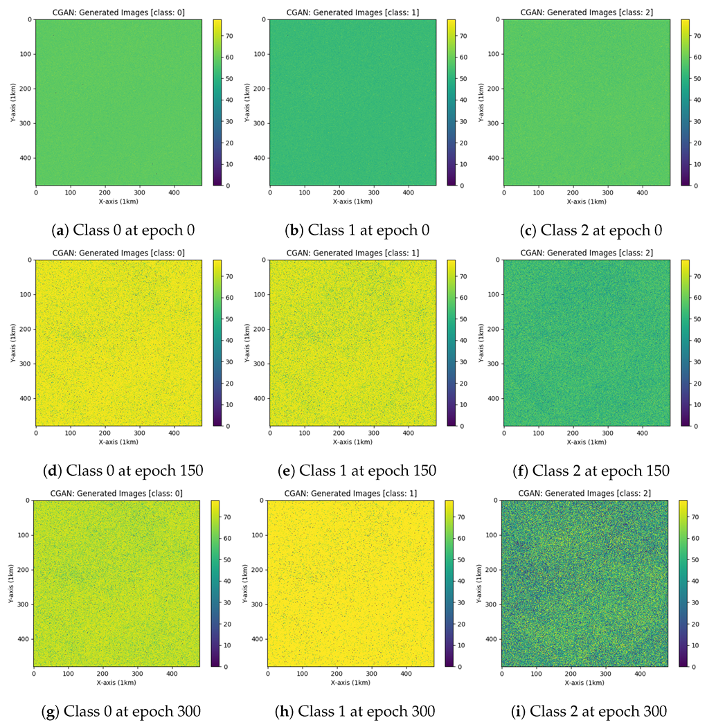
2.2. CGAN
2.3. DCGAN
2.4. InfoGAN
2.5. LSGAN
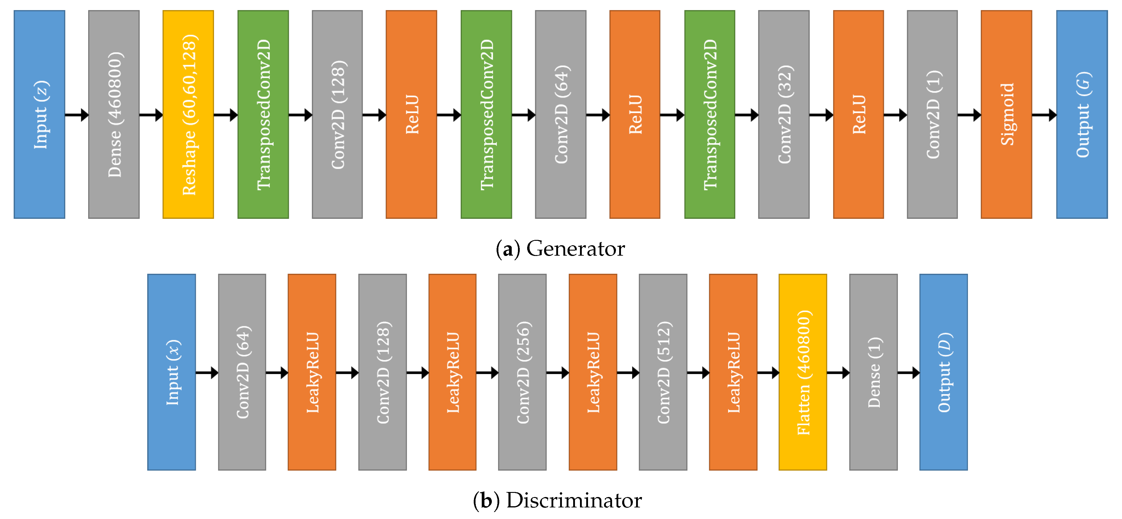
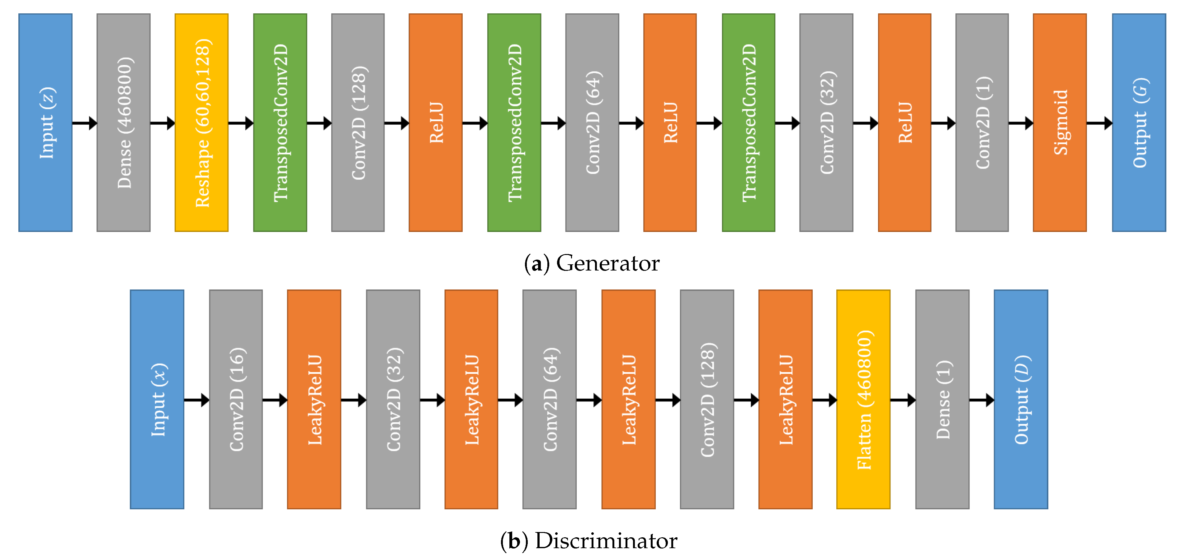
2.6. WGAN-GP
2.7. Image Quality Assessment
3. Results and Discussion
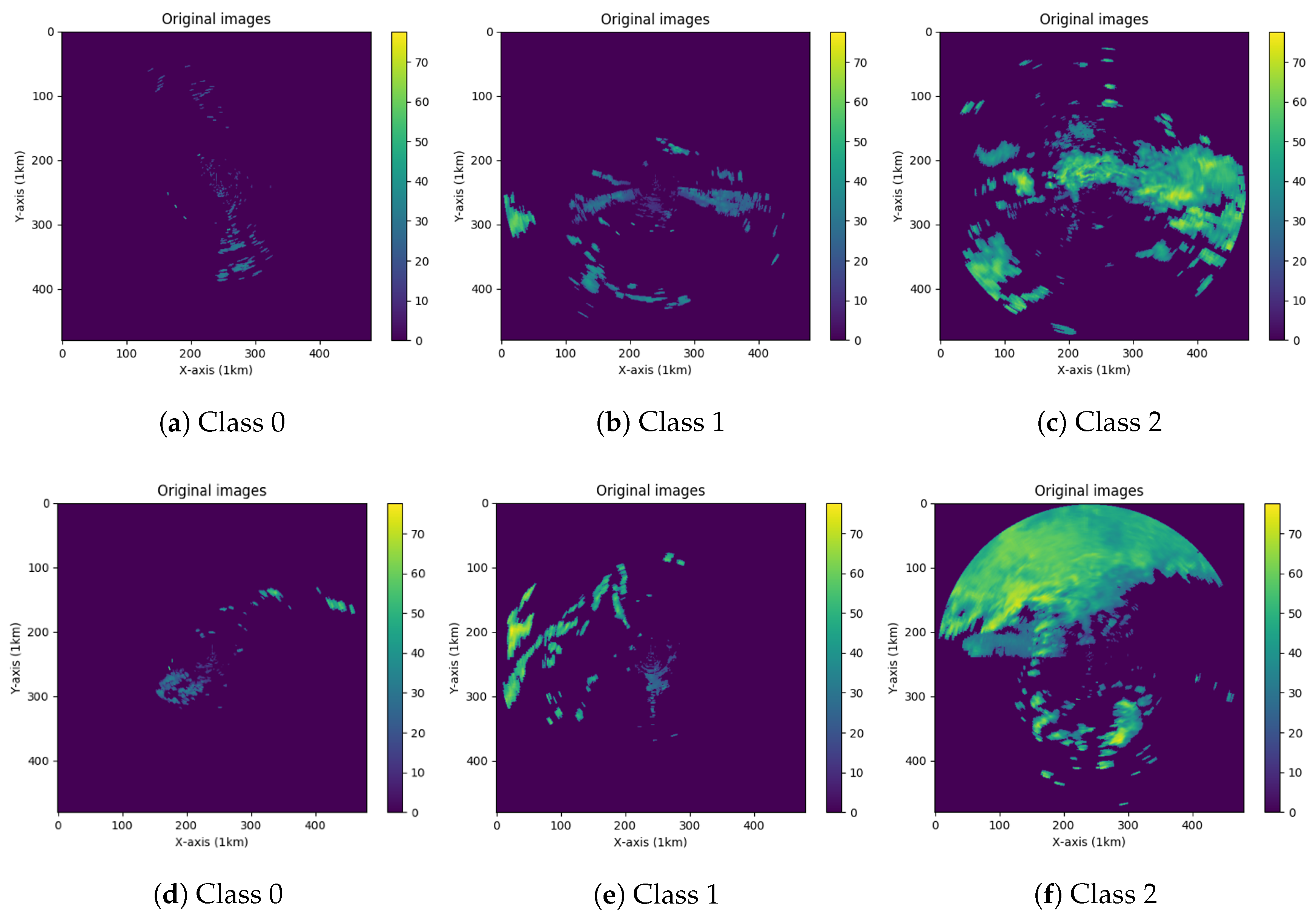
3.1. Data Description
3.2. Experiments
4. Conclusions
Author Contributions
Funding
Conflicts of Interest
References
- Tang, L.; Zhang, J.; Langston, C.; Krause, J.; Howard, K.; Lakshmanan, V. A physically based precipitation–nonprecipitation radar echo classifier using polarimetric and environmental data in a real-time national system. Weather. Forecast. 2014, 29, 1106–1119. [Google Scholar] [CrossRef]
- Han, L.; Fu, S.; Zhao, L.; Zheng, Y.; Wang, H.; Lin, Y. 3D convective storm identification, tracking, and forecasting—An enhanced TITAN algorithm. J. Atmos. Ocean. Technol. 2009, 26, 719–732. [Google Scholar] [CrossRef]
- Smith, T.M.; Elmore, K.L.; Dulin, S.A. A damaging downburst prediction and detection algorithm for the WSR-88D. Weather. Forecast. 2004, 19, 240–250. [Google Scholar] [CrossRef]
- Lakshmanan, V.; Herzog, B.; Kingfield, D. A method for extracting postevent storm tracks. J. Appl. Meteorol. Climatol. 2015, 54, 451–462. [Google Scholar] [CrossRef]
- Karimian, A.; Yardim, C.; Gerstoft, P.; Hodgkiss, W.S.; Barrios, A.E. Refractivity estimation from sea clutter: An invited review. Radio Sci. 2011, 46, 1–16. [Google Scholar] [CrossRef]
- Hubbert, J.; Dixon, M.; Ellis, S.; Meymaris, G. Weather radar ground clutter. Part I: Identification, modeling, and simulation. J. Atmos. Ocean. Technol. 2009, 26, 1165–1180. [Google Scholar] [CrossRef]
- Rico-Ramirez, M.A.; Cluckie, I.D. Classification of ground clutter and anomalous propagation using dual-polarization weather radar. IEEE Trans. Geosci. Remote. Sens. 2008, 46, 1892–1904. [Google Scholar] [CrossRef]
- Friedrich, K.; Hagen, M.; Einfalt, T. A quality control concept for radar reflectivity, polarimetric parameters, and Doppler velocity. J. Atmos. Ocean. Technol. 2006, 23, 865–887. [Google Scholar] [CrossRef]
- Lakshmanan, V.; Zhang, J.; Hondl, K.; Langston, C. A statistical approach to mitigating persistent clutter in radar reflectivity data. IEEE J. Sel. Top. Appl. Earth Obs. Remote. Sens. 2012, 5, 652–662. [Google Scholar] [CrossRef]
- Dufton, D.; Collier, C. Fuzzy logic filtering of radar reflectivity to remove non-meteorological echoes using dual polarization radar moments. Atmos. Meas. Tech. 2015, 8, 3985–4000. [Google Scholar] [CrossRef]
- Rennie, S.; Curtis, M.; Peter, J.; Seed, A.; Steinle, P.; Wen, G. Bayesian echo classification for Australian single-polarization weather radar with application to assimilation of radial velocity observations. J. Atmos. Ocean. Technol. 2015, 32, 1341–1355. [Google Scholar] [CrossRef]
- Medina, B.L.; Carey, L.D.; Amiot, C.G.; Mecikalski, R.M.; Roeder, W.P.; McNamara, T.M.; Blakeslee, R.J. A Random Forest Method to Forecast Downbursts Based on Dual-Polarization Radar Signatures. Remote. Sens. 2019, 11, 826. [Google Scholar] [CrossRef]
- Wen, G.; Protat, A.; Xiao, H. An objective prototype-based method for dual-polarization radar clutter identification. Atmosphere 2017, 8, 72. [Google Scholar] [CrossRef]
- LeCun, Y.; Bengio, Y.; Hinton, G. Deep learning. Nature 2015, 521, 436. [Google Scholar] [CrossRef] [PubMed]
- Lagerquist, R.; McGovern, A.; Smith, T. Machine learning for real-time prediction of damaging straight-line convective wind. Weather. Forecast. 2017, 32, 2175–2193. [Google Scholar] [CrossRef]
- Van Dyk, D.A.; Meng, X.L. The art of data augmentation. J. Comput. Graph. Stat. 2001, 10, 1–50. [Google Scholar] [CrossRef]
- Goodfellow, I.; Pouget-Abadie, J.; Mirza, M.; Xu, B.; Warde-Farley, D.; Ozair, S.; Courville, A.; Bengio, Y. Generative adversarial nets. In Proceedings of the Advances in Neural Information Processing Systems, Montreal, QC, Canada, 8–13 December 2014; pp. 2672–2680. [Google Scholar]
- Rajeswar, S.; Subramanian, S.; Dutil, F.; Pal, C.; Courville, A. Adversarial generation of natural language. arXiv 2017, arXiv:1705.10929. [Google Scholar]
- Zhu, L.; Chen, Y.; Ghamisi, P.; Benediktsson, J.A. Generative adversarial networks for hyperspectral image classification. IEEE Trans. Geosci. Remote. Sens. 2018, 56, 5046–5063. [Google Scholar] [CrossRef]
- Yi, X.; Walia, E.; Babyn, P. Generative adversarial network in medical imaging: A review. Med Image Anal. 2019, 101552. [Google Scholar] [CrossRef] [PubMed]
- Mirza, M.; Osindero, S. Conditional generative adversarial nets. arXiv 2014, arXiv:1411.1784. [Google Scholar]
- Radford, A.; Metz, L.; Chintala, S. Unsupervised representation learning with deep convolutional generative adversarial networks. arXiv 2015, arXiv:1511.06434. [Google Scholar]
- Chen, X.; Duan, Y.; Houthooft, R.; Schulman, J.; Sutskever, I.; Abbeel, P. Infogan: Interpretable representation learning by information maximizing generative adversarial nets. In Proceedings of the Advances in Neural Information Processing Systems, Barcelona, Spain, 5–10 December 2016; pp. 2172–2180. [Google Scholar]
- Mao, X.; Li, Q.; Xie, H.; Lau, R.Y.; Wang, Z.; Paul Smolley, S. Least squares generative adversarial networks. In Proceedings of the IEEE International Conference on Computer Vision, Venice, Italy, 22–29 October 2017; pp. 2794–2802. [Google Scholar]
- Arjovsky, M.; Chintala, S.; Bottou, L. Wasserstein generative adversarial networks. In Proceedings of the International Conference on Machine Learning, Sydney, Australia, 6–11 August 2017; pp. 214–223. [Google Scholar]
- Gulrajani, I.; Ahmed, F.; Arjovsky, M.; Dumoulin, V.; Courville, A.C. Improved training of wasserstein gans. In Proceedings of the Advances in Neural Information Processing Systems, Long Beach, CA, USA, 4–9 December 2017; pp. 5767–5777. [Google Scholar]
- Borji, A. Pros and cons of gan evaluation measures. Comput. Vis. Image Underst. 2019, 179, 41–65. [Google Scholar] [CrossRef]
- Wang, Z.; Bovik, A.C.; Sheikh, H.R.; Simoncelli, E.P. Image quality assessment: From error visibility to structural similarity. IEEE Trans. Image Process. 2004, 13, 600–612. [Google Scholar] [CrossRef] [PubMed]


| Original | GAN | CGAN | DCGAN | InfoGAN | LSGAN | WGAN-GP | |
|---|---|---|---|---|---|---|---|
| class 0 | case 1 (Figure 2a) | 0.1413 | 0.0002 | 0.0013 | 0.0007 | 0.0023 | 0.6245 |
| 0.1243 | 0.0003 | 0.0015 | 0.0006 | 0.0020 | 0.5687 | ||
| 0.1250 | 0.0002 | 0.0014 | 0.0006 | 0.0015 | 0.6022 | ||
| 0.1230 | 0.0002 | 0.0016 | 0.0007 | 0.0014 | 0.5455 | ||
| 0.1239 | 0.0002 | 0.0013 | 0.0007 | 0.0019 | 0.7570 | ||
| case 2 (Figure 2d) | 0.1349 | 0.0004 | 0.0025 | 0.0011 | 0.0025 | 0.5987 | |
| 0.1174 | 0.0003 | 0.0021 | 0.0010 | 0.0018 | 0.5436 | ||
| 0.1178 | 0.0005 | 0.0020 | 0.0010 | 0.0013 | 0.5792 | ||
| 0.1161 | 0.0004 | 0.0021 | 0.0012 | 0.0013 | 0.5262 | ||
| 0.1169 | 0.0004 | 0.0022 | 0.0011 | 0.0016 | 0.7401 | ||
| class 1 | case 1 (Figure 2b) | 0.0058 | 0.0024 | 0.0073 | 0.0050 | 0.0068 | 0.5306 |
| 0.0091 | 0.0027 | 0.0078 | 0.0063 | 0.0073 | 0.4792 | ||
| 0.0097 | 0.0019 | 0.0064 | 0.0068 | 0.0069 | 0.4848 | ||
| 0.0136 | 0.0023 | 0.0073 | 0.0059 | 0.0086 | 0.4778 | ||
| 0.0034 | 0.0008 | 0.0061 | 0.0062 | 0.0073 | 0.4471 | ||
| case 2 (Figure 2e) | 0.0038 | 0.0016 | 0.0083 | 0.0061 | 0.0040 | 0.4424 | |
| 0.0076 | 0.0024 | 0.0089 | 0.0061 | 0.0049 | 0.4803 | ||
| 0.0082 | 0.0012 | 0.0073 | 0.0065 | 0.0038 | 0.4379 | ||
| 0.0122 | 0.0016 | 0.0068 | 0.0062 | 0.0056 | 0.4258 | ||
| 0.0012 | 0.0027 | 0.0063 | 0.0058 | 0.0044 | 0.4054 | ||
| class 2 | case 1 (Figure 2c) | 0.0017 | 0.0151 | 0.0314 | 0.0468 | 0.0332 | 0.2584 |
| 0.0064 | 0.0116 | 0.0330 | 0.0453 | 0.0252 | 0.3878 | ||
| 0.0074 | 0.0077 | 0.0460 | 0.0450 | 0.0358 | 0.3425 | ||
| 0.0116 | 0.0086 | 0.0389 | 0.0429 | 0.0318 | 0.3322 | ||
| 0.0088 | 0.0095 | 0.0431 | 0.0426 | 0.0333 | 0.3127 | ||
| case 2 (Figure 2f) | 0.0387 | 0.0045 | 0.0876 | 0.1255 | 0.0899 | 0.3138 | |
| 0.0130 | 0.0136 | 0.0975 | 0.1197 | 0.0876 | 0.3962 | ||
| 0.0168 | 0.0158 | 0.1106 | 0.1164 | 0.0777 | 0.3422 | ||
| 0.0248 | 0.0048 | 0.1039 | 0.1215 | 0.0805 | 0.3118 | ||
| 0.0205 | 0.0194 | 0.1154 | 0.1129 | 0.0790 | 0.3106 |
| GAN | CGAN | DCGAN | InfoGAN | LSGAN | WGAN-GP | |
|---|---|---|---|---|---|---|
| Time | 27,930 s | 28,364 s | 42,950 s | 62,843 s | 42,893 s | 464 s |
© 2020 by the authors. Licensee MDPI, Basel, Switzerland. This article is an open access article distributed under the terms and conditions of the Creative Commons Attribution (CC BY) license (http://creativecommons.org/licenses/by/4.0/).
Share and Cite
Lee, H.; Kim, J.; Kim, E.K.; Kim, S. Wasserstein Generative Adversarial Networks Based Data Augmentation for Radar Data Analysis. Appl. Sci. 2020, 10, 1449. https://doi.org/10.3390/app10041449
Lee H, Kim J, Kim EK, Kim S. Wasserstein Generative Adversarial Networks Based Data Augmentation for Radar Data Analysis. Applied Sciences. 2020; 10(4):1449. https://doi.org/10.3390/app10041449
Chicago/Turabian StyleLee, Hansoo, Jonggeun Kim, Eun Kyeong Kim, and Sungshin Kim. 2020. "Wasserstein Generative Adversarial Networks Based Data Augmentation for Radar Data Analysis" Applied Sciences 10, no. 4: 1449. https://doi.org/10.3390/app10041449
APA StyleLee, H., Kim, J., Kim, E. K., & Kim, S. (2020). Wasserstein Generative Adversarial Networks Based Data Augmentation for Radar Data Analysis. Applied Sciences, 10(4), 1449. https://doi.org/10.3390/app10041449