Numerical Simulation of Ship Oil Spill in Arctic Icy Waters


Abstract
:Featured Application
Abstract
1. Introduction
2. Modelling Methods
2.1. VOF Method
2.2. Discrete Element Method (DEM)
2.3. Eulerian–Lagrangian Method
3. Numerical Simulation of Oil Spill
3.1. Simulation of Oil-Spill Drift
3.2. Simulation of Ice-Floes Drift
3.3. Numerical Model
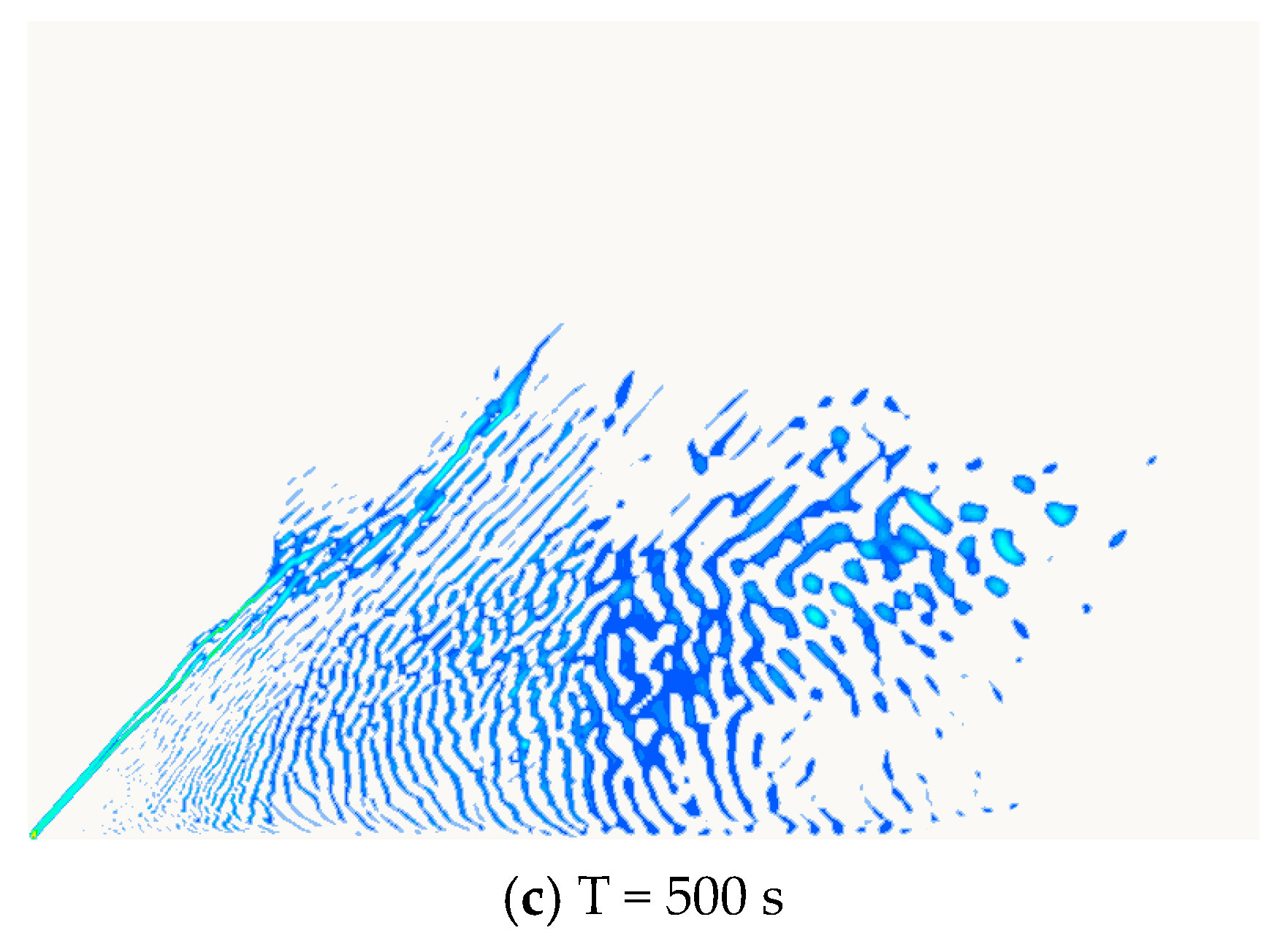
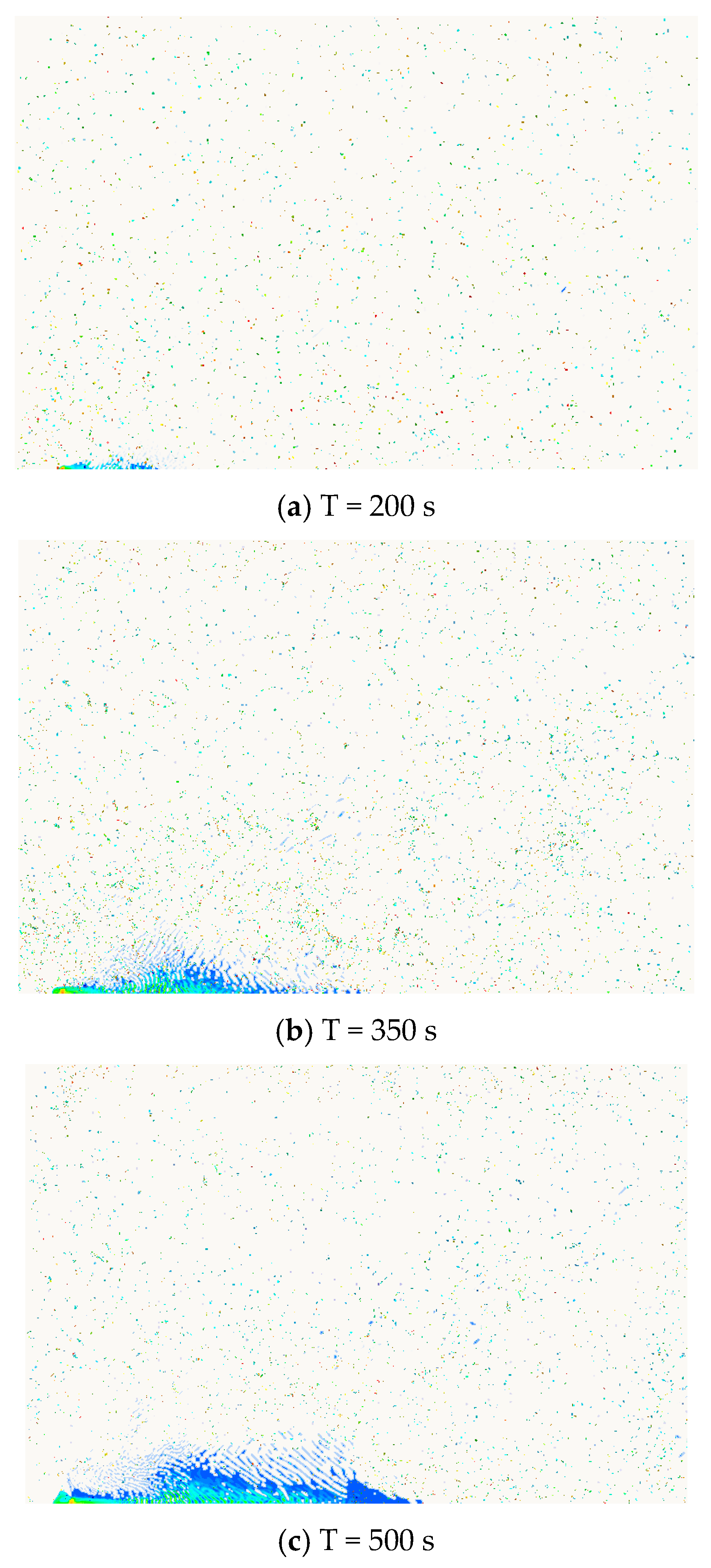
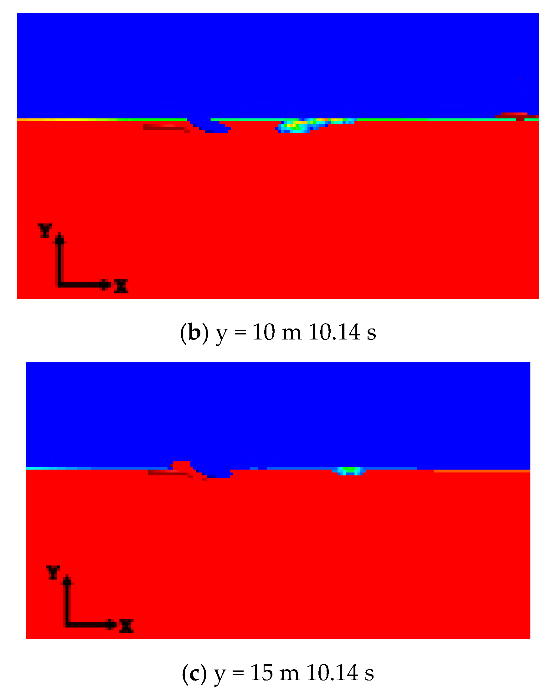
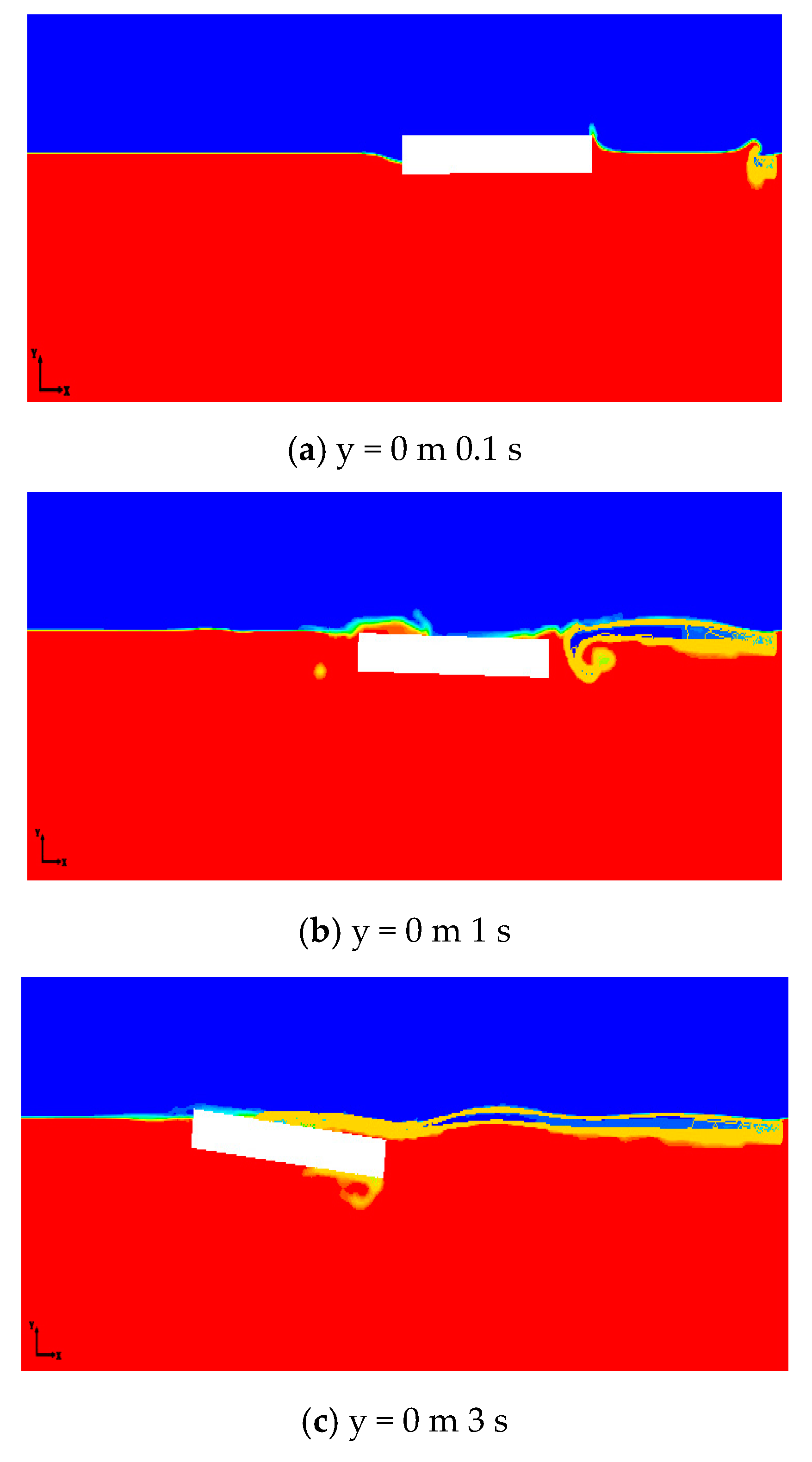
3.4. Characteristics of Oil Spill in Icy and Ice-Free Waters
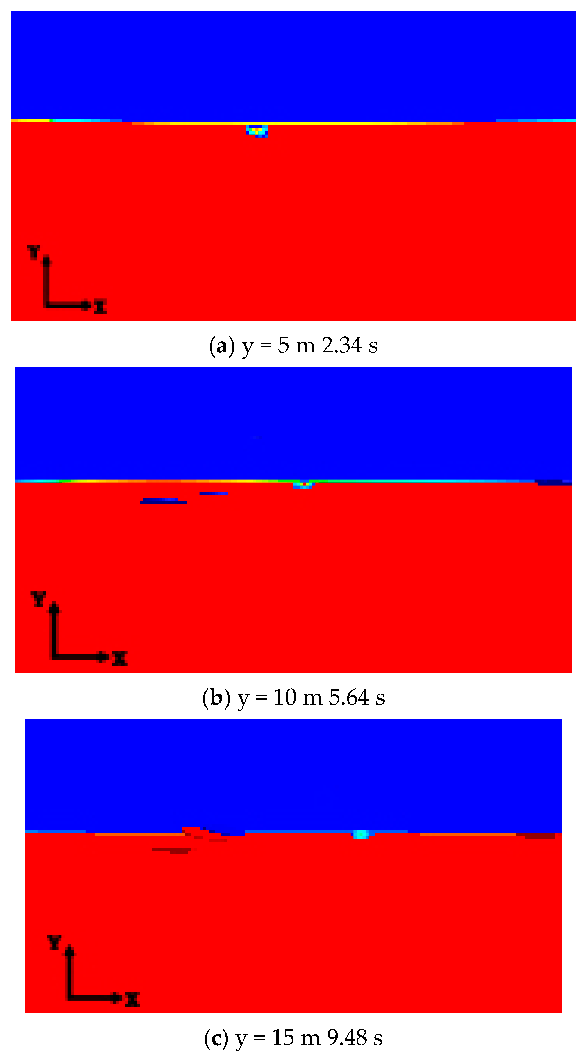
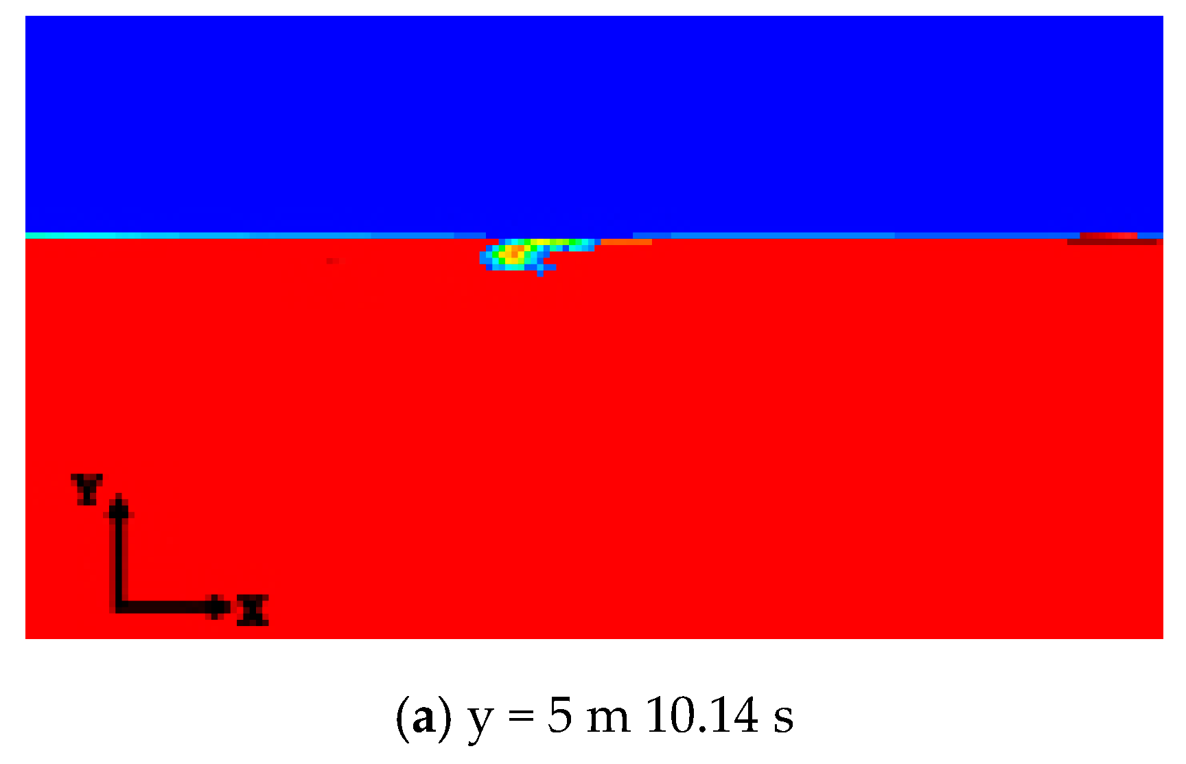
3.5. Interaction of Ice and Oil
4. Prediction of Oil-Spill Pollution Area
- 1.
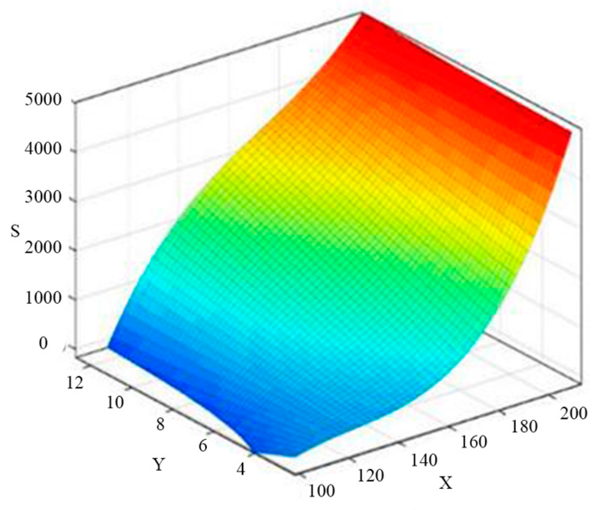
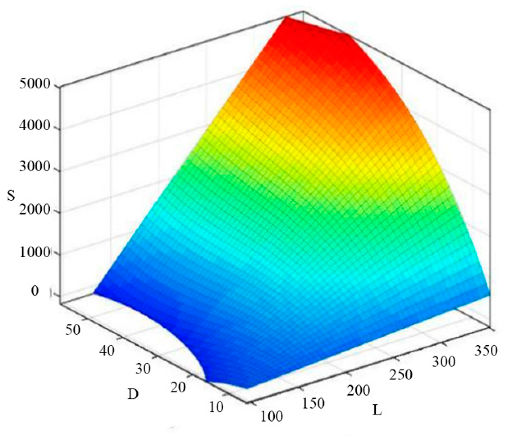
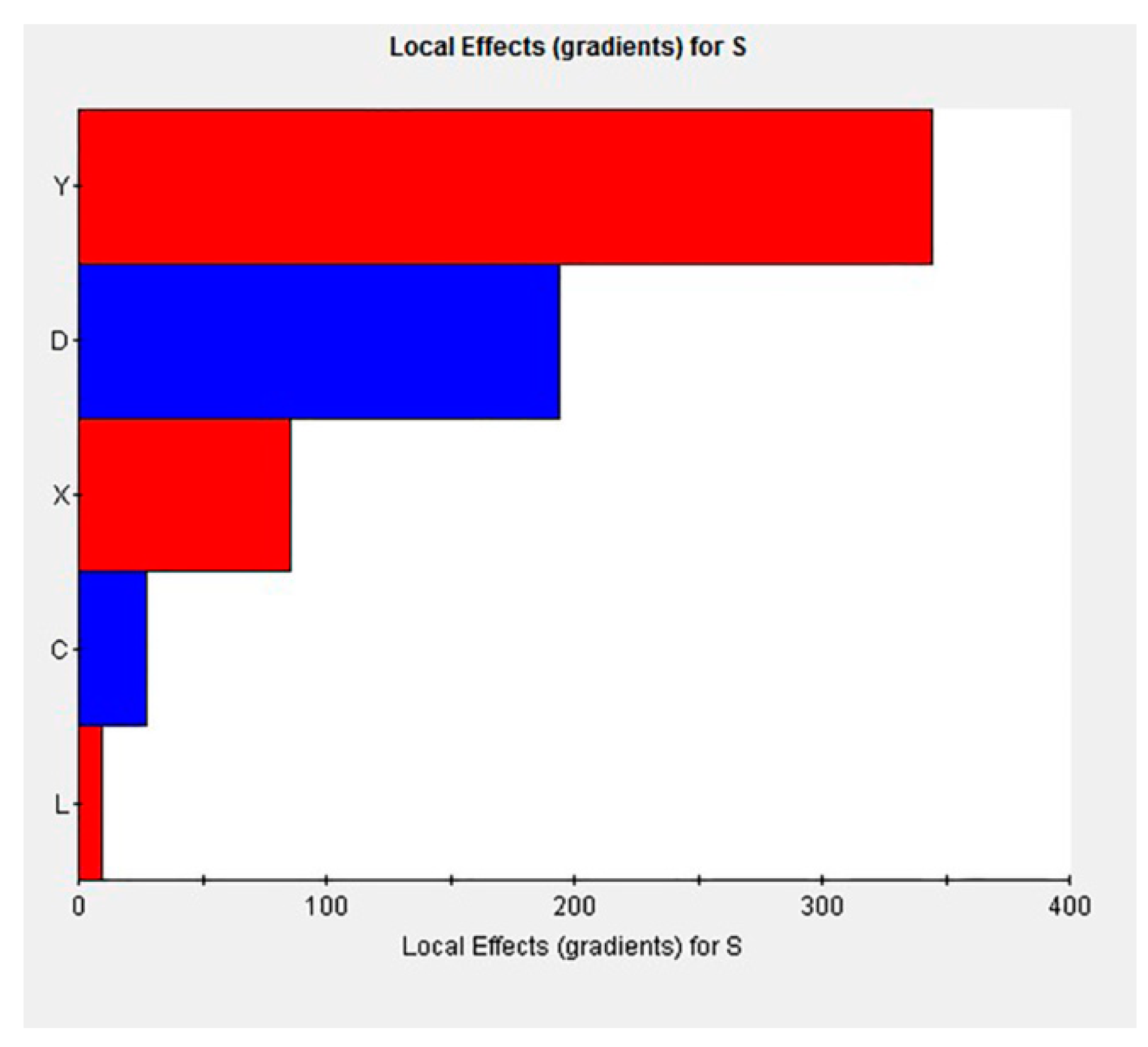
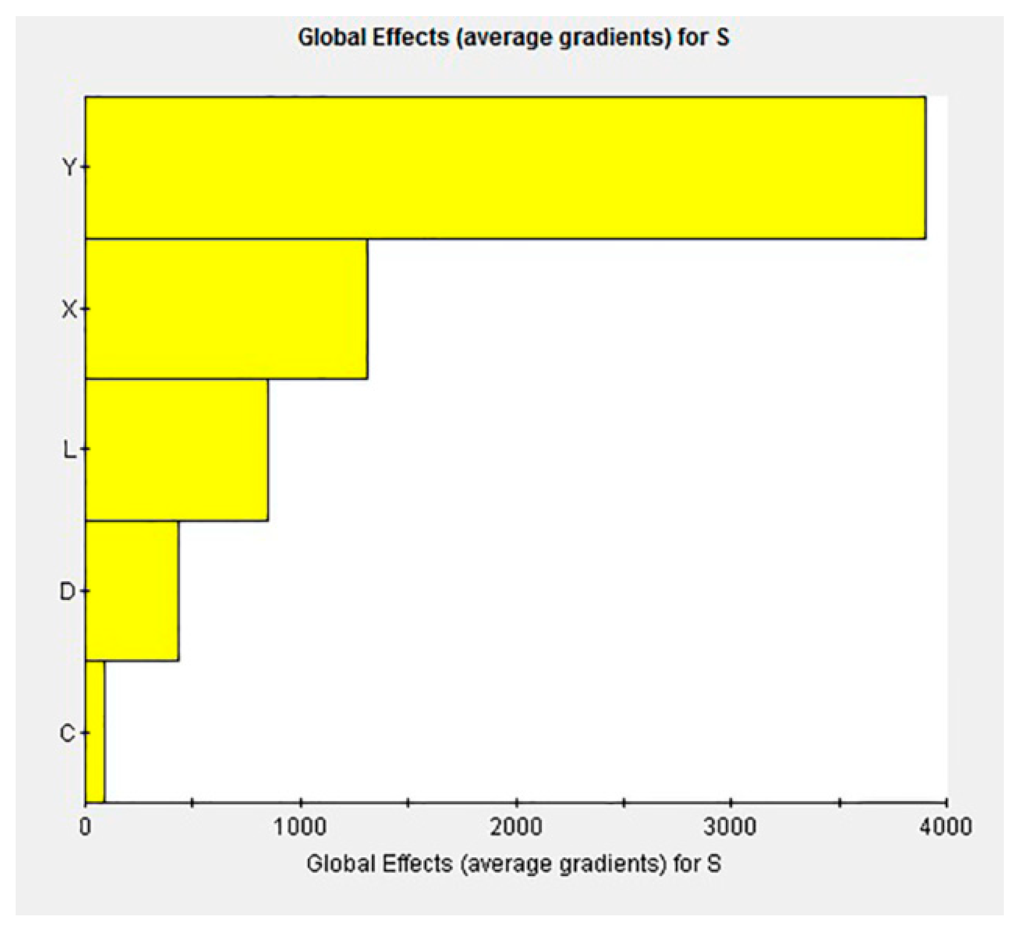
- The sample point was determined to construct the approximate model in the design space using the experimental design methodology, where and m was the number of design variables. The data of sample points were the centroid coordinates (X, Y), area S, perimeter C’, horizontal maximum distance L and vertical maximum distance D of the contaminated area, which were extracted from the numerical results of oil spill diffusion at different times as presented in Section 3.4 (i.e., 40 s, 80 s, 120 s, 160 s, and 200 s).
- 2.
- A series of sample pairs of designated variables and responses were computed by the model, where was the response of the oil-spill area, and n was the number of sample points designed for the test.
- 3.
- The regression analysis using RSM was conducted to obtain an approximate model of the oil-spill area. The multiple correlation coefficient was adopted to evaluate the credibility of the response surface model. If the requirements were met, this model could be applied to the subsequent optimization computation. Otherwise, the credibility of the model could be improved by changing the model type and increasing the sample points.
5. Conclusions
- 1.
- The presence of ice floes had a significant suppression effect on the movement of the oil spill. The maximum drift distance of oil film and the maximum radius of oil diffusion in icy waters were found to be much smaller than those in open waters. With the combined action of wind, wave, current and ice, the oil film was observed to expand to a larger area in ice-free waters but form a long and narrow belt in icy waters.
- 2.
- The oil film diffusion and drift processes occurred simultaneously. The oil film in waters with medium-density ice was observed to be distributed on both the water surface and underwater. The underwater oil gradually rose until it came into contact with the ice, and then spread to the surroundings. The changes in the horizontal drift distance of the oil spill were more evident than those in oil-film thickness. Thus, oil-film drift constituted the primary behavior of oil-spill expansion.
- 3.
- The regression function of time t, the centroid coordinates (X, Y), perimeter C’, horizontal maximum distance L and vertical maximum distance D were generated on the base of the approximate model method. This function exhibited a relatively high degree of credibility. It could predict the extent of oil spill in icy waters scientifically and reasonably, which could provide support for establishing a rapid emergency oil-spill cleanup system in icy waters, such as those found in the increasingly accessible Arctic Ocean.
Author Contributions
Funding
Conflicts of Interest
Abbreviations
| DPM | Discrete Phase Model |
| DEM | Discrete Element Method |
| RSM | Response Surface Method |
| VOF | Volume of Fluid Method |
| 6DOF | Six Degrees of Freedom |
Notations
| Velocity component of fluid in x direction | |
| Velocity component of fluid in y direction | |
| Flow time | |
| Ratio of the volume of q-th phase fluid in the cell to the total cell volume | |
| Fluid parameter | |
| Normal contact force at time | |
| Normal contact stiffness | |
| Contact viscous coefficient | |
| Overlap value between the two disks and | |
| Relative velocity vector of the contact faces | |
| Normal unit vector of the contact cells | |
| Tangential forces at time | |
| Tangential forces at time | |
| Tangential stiffness between particles | |
| Time step | |
| Tangential unit vector between contact cells | |
| Coefficient of sliding friction | |
| Concentration | |
| Vertical diffusion coefficient | |
| Horizontal diffusion coefficient | |
| Position of the marked substance micelle at time | |
| Normal coordinates | |
| Number of cells in the computational domain | |
| Volume occupied by the particles on the ocean surface in grid cell | |
| Shear stresses of the wind in the direction | |
| Shear stresses of the wind in the direction | |
| Diffusion coefficient of the oil film | |
| Friction coefficient of the oil–water interface | |
| Acceleration due to gravity | |
| Physical–chemical kinetic terms | |
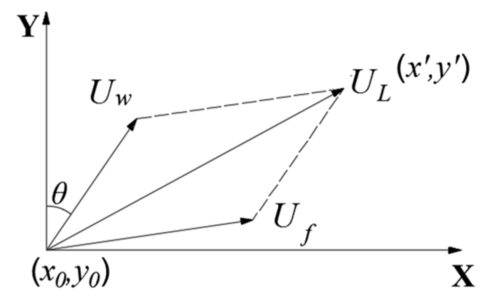
| Initial position of the oil-film centroid | |
| New position of the oil-film centroid after a time | |
| Velocity of oil-film drift | |
| Velocity on water surface | |
| Velocity of wind | |
| Horizontal flow coefficient | |
| Wind frag coefficient | |
| , | Initial centroid position |
| , | Centroid position after a time |
| Current velocity in the direction | |
| Current velocity in the direction | |
| Correction factor | |
| Wind angle | |
| Coriolis force | |
| Force of the wind above ice floe | |
| Force of the current above ice floe | |
| Effects of the ocean surface slope | |
| Non-linear ice internal force | |
| Gravitational potential on the ocean surface | |
| Coriolis force coefficient | |
| Unit vector perpendicular to the ocean surface | |
| Velocity of the ice floe | |
| Ice density | |
| Average ice thickness in the grid | |
| Unit area mass of ice floe | |
| Thermodynamic term determined by ice thickness | |
| Thermodynamic term determined by ice density | |
| Response of a sample point | |
| Response of an approximate model | |
| Design parameter value | |
| Number of designated parameters; | |
| Error between the response value and true value | |
| S | Area of oil film |
| C’ | Perimeter of oil film |
| L | Horizontal maximum distance of oil film |
| D | Vertical maximum distance of oil film |
| Sample numbers | |
| Real value of simulation program | |
| Estimated value of response surface model | |
| Mean of true response |
References
- Pietri, D.; Soule, A.B.; Kershner, J.; Soles, P.; Sullivan, M. The arctic shipping and environmental management agreement: A regime for marine pollution. Coast. Manag. 2008, 36, 508–523. [Google Scholar] [CrossRef]
- Eide, M.S.; Endresen, O.; Breivik, O.; Brude, O.W.; Ellingsen, I.H.; Røang, K.; Hauge, J.; Brett, P.O. Prevention of oil spill from shipping by modelling of dynamic risk. Mar. Pollut. Bull. 2007, 54, 1619–1633. [Google Scholar] [CrossRef]
- Shiau, B.S.; Tsai, R.S. A numerical simulation of oil spill spreading on the coastal waters. J. Chin. Inst. Eng. 1994, 17, 473–484. [Google Scholar] [CrossRef]
- Johansen, Ø. DeepBlow—A Lagrangian Plume Model for Deep Water Blowouts. Spill Sci. Technol. Bull. 2000, 6, 103–111. [Google Scholar] [CrossRef]
- Yapa, P.D.; Li, Z. Simulation of oil spills from underwater accidents I: Model development. J. Hydraul. Res. 1998, 35, 673–688. [Google Scholar] [CrossRef]
- Wang, P.; Li, Z.J. A Primary Numerical Model of Oil Spilling in Icing Sea. J. Glaciol. Geocryol. 2003, 25, 334–337. [Google Scholar]
- Chen, X.; Yu, J.X.; Li, Z.G.; Wu, C.H.; Jiang, M.R.; Yang, Z.L. Application of Discrete Phase Model and Empirical Model in Oil Spill Simulation of Sea Surface. China Offshore Platf. 2019, 34, 47–53. [Google Scholar]
- Ambjorn, C. Seatrack Web, Forecasts of Oil Spills, a New Version. Environ. Res. Eng. Manag. 2007, 41, 60–66. [Google Scholar]
- Venkatesh, S.; El-Tahan, H.; Comfort, G.; Abdelnour, R. Modelling the behaviour of oil spills in ice-infested waters. Atmos. Ocean 1990, 28, 303–329. [Google Scholar] [CrossRef]
- Wang, R.S.; Liu, Q.Z.; Chen, W.B.; Jin, H.T.; Liu, C.H. Numerical simulation and tests of sea ice drift process in the bohai sea. Oceanol. Limnol. Sin. 1994, 3, 10. [Google Scholar]
- Xia, D.W.; Xu, J.Z. Investigation on numerical modelling of spill oil movement in sea ice infested waters. Acta Oceanol. Sin. 1998, 1, 113–122. [Google Scholar]
- Huang, J.; Cao, Y.J.; Gao, S. Numerical simulation of oil spill drift-diffusion in the Bohai sea. Mar. Sci. 2014, 38, 100–107. [Google Scholar]
- Huang, Y.; Song, M.R.; Guan, P. Study on the Varying Regularity of Oil Spill Properties During the Ice Period of the Bohai Sea. J. Ocean Technol. 2016, 35, 1–5. [Google Scholar]
- Yu, J.A.; Zhang, B.; Liu, Q.Z.; Chen, W.B.; Wang, R.S. Numerical experiment on the behaviour of oil spills in ice-infested waters in the bohai sea. Oceanol. Limnol. Sin. 1999, 30, 557–562. [Google Scholar]
- Wilkinson, J.P.; Wadhams, P.; Hughes, N.E. Modelling the spread of oil under fast sea ice using three-dimensional multibeam sonar data. Geophys. Res. Lett. 2007, 34, L22506. [Google Scholar] [CrossRef]
- Xiao, M.; Gao, Q.J.; Lin, J.G.; Li, W.; Liang, X. Simulation of Submarine Pipeline Oil Spill Based on Wave Motion. In Proceedings of the International Conference on Computer Modeling and Simulation, Hainan, China, 22–24 January 2010; Volume 1, pp. 433–437. [Google Scholar]
- Liu, X.F.; Meng, L.K.; Zhao, C.Y. DEM-based Oil and Gas Migration Pathway Simulation of Oil-and Gas-Bearing Basin. Editor. Board Geomat. Inf. Sci. Wuhan Univ. 2004, 29, 371–375. [Google Scholar]
- Ma, E.; Xu, Z.M. Technological process and optimum design of organic materials vacuum pyrolysis and indium chlorinated separation from waste liquid crystal display panels. J. Hazard. Mater. 2013, 263, 610–617. [Google Scholar] [CrossRef]
- Lv, G.L.; Liu, Z.M. Simulation and Analysis of Diffusion of Oil and Gas Leakage from Submarine Pipeline Based on CFD. J. Jimei Univ. 2017, 22, 51–57. [Google Scholar]
- Ren, B.; Li, X.L.; Wang, Y.X. An Irregular Wave Maker of Active Absorption with VOF Method. China Ocean Eng. 2008, 4, 94–105. [Google Scholar]
- Li, Z.G.; Jiang, M.R.; Yu, J.X. Numerical simulation on the oil spill for the submarine pipeline based on VOF method. Ocean Eng. 2016, 34, 100–110. [Google Scholar]
- Li, Z.L.; Liu, Y.; Sun, S.S.; Lu, Y.L.; Ji, S.Y. Analysis of ship maneuvering performances and ice loads on ship hull with discrete element model in broken-ice fields. Chin. J. Theor. Appl. Mech. 2013, 45, 868–877. [Google Scholar]
- Mohr, O. Welche Umstande bedingen die Elastizitatsgrenze undden bruch eines materials. Z. Des. Ver. Dtsch. Ing. 1900, 44, 1524–1530. [Google Scholar]
- Egberongbe, F.O.; Nwilo, P.C.; Badejo, O.T. Oil Spill Disaster Monitoring along Nigerian Coastline. In Proceedings of the 5th FIG Regional Conference: Promoting Land Administration and Good Governance, Accra, Ghana, 8–11 March 2006. [Google Scholar]
- Cheng, R.T.; Casulli, V.; Milford, S.N. Eulerian-Lagrangian Solution of the Convection-Dispersion Equation in Natural Coordinates. Water Resour. Res. 1984, 20, 944–952. [Google Scholar] [CrossRef]
- Yang, Z.Y. B-Spline interpolation in Eular-Lagrangian method for convection-dispersion equation. J. Ocean Univ. Qingdao 1994, 2, 143–151. [Google Scholar]
- Rasmussen, T.L.; Thomsen, E.; Kuijpers, A.; Stefan, W. Late warming and early cooling of the sea surface in the Nordic seas during MIS 5e (Eemian Interglacial). Quat. Sci. Rev. 2003, 22, 809–821. [Google Scholar] [CrossRef]
- DF Dickins Associates. Field Research Spills to Investigate the Physical and Chemical Fate of Oil in Pack Ice; Environmental Studies Revolving Funds: Canada, 1987; 118p. [Google Scholar]
- Sun, H.; Lu, P.; Li, Z.J. Numerical Simulation on Dynamic Characteristics of Flow Field under Ice. Math. Pract. Theory 2015, 45, 69–77. [Google Scholar]
- Tu, X.C. Ice Resistance Prediction and Parameters Sensitivity Study for Polar Geophysical Prospecting Vessel. Master Thesis, Jiangsu University of Science and Technology, Zhenjiang, China, 2019. [Google Scholar]
- Ma, S.; Ge, W.P.; Duan, W.Y.; Liu, H.X. Simulation of free decay roll for C11 container ship based on overset gird. J. Huazhong Univ. Sci. Technol. 2017, 45, 34–39. [Google Scholar]
- Li, Y.; Liu, B.X.; Lan, G.X.; Ma, L.; Gao, C. Study on Spectrum of Oil Film in Ice-Infested Waters. Guang Pu Xue Yu Guang Pu Fen Xi 2010, 30, 1018–1021. [Google Scholar]


| Properties | Parameters |
|---|---|
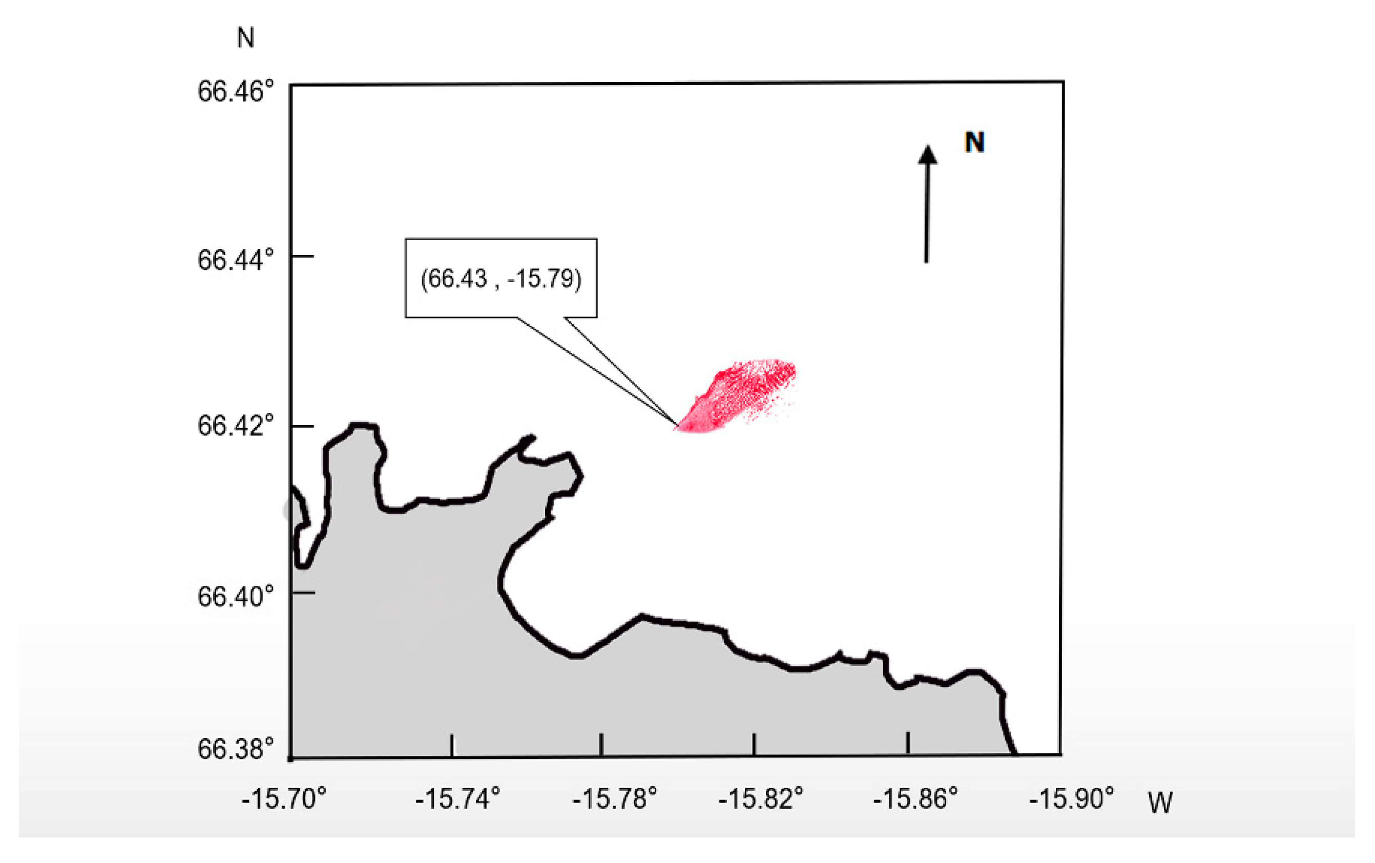
| Location | 66.43° N, 15.79° W |
| Release situation | Accidental ship leakage |
| Spill rate | 15 kg/s |
| Spill duration | 200 s |
| Oil density | 840 kg/m3 |
| Oil viscosity | 500 mPa·s |
| seawater density | 1025 kg/m3 |
| ice density | 910 kg/m3 |
| Ice diameter | 5 m |
| Ice concentration | Medium (30–80%) |
| Position of y/m | Time(t)/s | Width of the Oil Film/m | Thickness of the Oil Film/m |
|---|---|---|---|
| y = 5 | 2.34–10.14 | 2.67–6.46 | 1.82–1.99 |
| y = 10 | 5.64–10.14 | 2.96–9.51 | 1.44–1.94 |
| y = 15 | 9.48–10.14 | 2.72–4.10 | 1.23–1.34 |
| Time(t) /s | ||||||
|---|---|---|---|---|---|---|
| 5 | 65.33 | 40.88 | 103.99 | 3.09 | 108.06 | 7.28 |
| 10 | 100.23 | 41.6 | 104.01 | 3.14 | 111.91 | 7.5 |
| 20 | 214.91 | 63.75 | 109.16 | 4.5 | 121.7 | 12.05 |
| 25 | 331.59 | 86.64 | 113.91 | 4.93 | 130.03 | 13.23 |
| 30 | 354.71 | 95.52 | 116.56 | 4.46 | 135.42 | 11.73 |
| 40 | 476.29 | 121.62 | 123 | 4.31 | 149.24 | 11.76 |
| 50 | 500.27 | 148.83 | 128.49 | 2.75 | 162.32 | 8.27 |
| 60 | 524.14 | 186.14 | 133.57 | 2.56 | 181.61 | 9.08 |
| 70 | 772.1 | 236.14 | 143.35 | 2.71 | 207.39 | 10.28 |
| 75 | 775.34 | 254.93 | 145.48 | 3.61 | 208.27 | 11.01 |
| 80 | 1138.79 | 302.18 | 154.09 | 4.98 | 224.39 | 15.93 |
| 90 | 1173.98 | 309.93 | 145.95 | 5.33 | 220.1 | 17.39 |
| 95 | 1262.44 | 346.96 | 147.97 | 6.16 | 220.89 | 21.58 |
| 100 | 1535.68 | 351.8 | 152.47 | 7.63 | 222.3 | 28.44 |
| 110 | 1618.11 | 408.45 | 151.36 | 7.93 | 222.72 | 30.97 |
| 120 | 2236.59 | 484.88 | 162.31 | 9.24 | 242.96 | 35.7 |
| 125 | 2291.43 | 454.33 | 168.08 | 8.13 | 251.08 | 32.12 |
| 130 | 2369.06 | 474.85 | 168.84 | 7.27 | 256.49 | 29.33 |
| 140 | 2423.48 | 432.39 | 176.93 | 6.63 | 266.22 | 24.62 |
| 150 | 2819.96 | 489.75 | 181.67 | 6.85 | 285.7 | 29.66 |
| 160 | 3344.54 | 690.65 | 173.01 | 11.14 | 270.35 | 55.5 |
| 170 | 3415.69 | 703.94 | 189.05 | 10.32 | 288 | 38.41 |
| 175 | 3674.69 | 883.42 | 190.71 | 11.51 | 306.49 | 45.38 |
| 180 | 3943.54 | 987.46 | 194.54 | 12.25 | 308.54 | 44.42 |
| 190 | 4225.53 | 942.32 | 202.43 | 10.35 | 338.16 | 41.04 |
| 195 | 4361.73 | 727.68 | 200.25 | 11.74 | 315.29 | 43.76 |
| 200 | 4792.95 | 707.69 | 207.89 | 10.7 | 340.31 | 41.7 |
© 2020 by the authors. Licensee MDPI, Basel, Switzerland. This article is an open access article distributed under the terms and conditions of the Creative Commons Attribution (CC BY) license (http://creativecommons.org/licenses/by/4.0/).
Share and Cite
Li, W.; Liang, X.; Lin, J.; Guo, P.; Ma, Q.; Dong, Z.; Liu, J.; Song, Z.; Wang, H. Numerical Simulation of Ship Oil Spill in Arctic Icy Waters. Appl. Sci. 2020, 10, 1394. https://doi.org/10.3390/app10041394
Li W, Liang X, Lin J, Guo P, Ma Q, Dong Z, Liu J, Song Z, Wang H. Numerical Simulation of Ship Oil Spill in Arctic Icy Waters. Applied Sciences. 2020; 10(4):1394. https://doi.org/10.3390/app10041394
Chicago/Turabian StyleLi, Wei, Xiao Liang, Jianguo Lin, Ping Guo, Qiang Ma, Zhenpeng Dong, Jiamin Liu, Zhenhe Song, and Hengqi Wang. 2020. "Numerical Simulation of Ship Oil Spill in Arctic Icy Waters" Applied Sciences 10, no. 4: 1394. https://doi.org/10.3390/app10041394
APA StyleLi, W., Liang, X., Lin, J., Guo, P., Ma, Q., Dong, Z., Liu, J., Song, Z., & Wang, H. (2020). Numerical Simulation of Ship Oil Spill in Arctic Icy Waters. Applied Sciences, 10(4), 1394. https://doi.org/10.3390/app10041394