Article

Deep Learning for Computational Mode Decomposition in Optical Fibers

Chair of Measurement and Sensor System Technique, Technische Universität Dresden, Helmholtzstraße 18, 01069 Dresden, Germany
*
Author to whom correspondence should be addressed.
Appl. Sci. 2020, 10(4), 1367; https://doi.org/10.3390/app10041367
Submission received: 22 January 2020 / Revised: 13 February 2020 / Accepted: 15 February 2020 / Published: 18 February 2020

Abstract

:
Multimode fibers are regarded as the key technology for the steady increase in data rates in optical communication. However, light propagation in multimode fibers is complex and can lead to distortions in the transmission of information. Therefore, strategies to control the propagation of light should be developed. These strategies include the measurement of the amplitude and phase of the light field after propagation through the fiber. This is usually done with holographic approaches. In this paper, we discuss the use of a deep neural network to determine the amplitude and phase information from simple intensity-only camera images. A new type of training was developed, which is much more robust and precise than conventional training data designs. We show that the performance of the deep neural network is comparable to digital holography, but requires significantly smaller efforts. The fast characterization of multimode fibers is particularly suitable for high-performance applications like cyberphysical systems in the internet of things.

1. Introduction

Optical fibers are used in a variety of applications. On the one hand, they are used in biophotonics as an image transmitting device [1,2]. On the other hand, multimode optical fibers (MMF) are also used in information technology, where the high number of modes permits spatial multiplexing. The basic idea is to transmit the eigenmodes of the optical fiber in order to obtain a Multiple-Input Multiple-Output (MIMO) transmission system with only one single fiber. Mode division multiplexing is said to be the next key development for increasing possible transmission rates [3]. However, light propagation through an MMF is nontrivial: a coherent light signal launched into an MMF exits as a speckle pattern due to mode-mixing effects [4]. These arise from two major sources. First, angle deviations occur during light injection; second, external parameters such as temperature fluctuations, mechanical stress (bending or twisting), and manufacturing tolerances have a considerable influence on the light transmission. For a long time, this made MMFs unsuitable for laser-based applications. However, due to the technological and methodological development, methods have been demonstrated that allow compensating and controlling the light distortions from the MMFs. While the first works were based on analogue holography approaches [5], in recent years, digital holography and wavefront shaping have shown a tremendous potential [6]. Iterative optimization [7,8], digital optical phase conjugation [9,10,11], or the transmission matrix (T) method [12] were developed to control the light transmission of an MMF even in “real time”. For the transmission of complex patterns in the fields of biophotonics and communications engineering, the T method has proven its worth [13,14,15,16]. The complex-valued weights of T link the modes, excited at the MMF input, with those that exit the MMF. With complete knowledge of the T method, it is thus possible to generate arbitrary structures at the output of the MMF, limited by the degrees of freedom of the MMF’s mode domain. Measurement of the T requires a complex analysis of the light field at the MMF. The light field leaving the MMF is a superposition consisting of the light-field distributions of the modes, which are contained in the finite mode domain of the MMF. An extremely reliable measurement technique that performs mode analysis in an MMF is S 2 imaging [17]. However, since S 2 imaging is a scanning method, it is not suitable for the intended application in the field of MIMO communication technology [18], as this requires a single-shot mode decomposition (MD).
In previous work, the author has shown a technique based on Digital Holography (DH) with which complex-valued MMF speckle patterns can be reconstructed and decomposed into the individual mode components by means of an orthogonal series expansion [19]. However, digital holographic techniques have the drawbacks that they are prone to environmental perturbations and phase instabilities [20,21] and that a reference beam is required. In optical data transmission, this would mean that an additional single-mode fiber has to be used carrying the coherent reference beam, which is impractical. A possible solution to this problem could be to tailor a reference beam using self-referencing. Here, the object beam is duplicated and optically processed to generate the reference beam [22]. However, it is not straightforward to apply this approach to the introduced MD problem, as an adaptive pinhole would be required. For this reason, it is preferable to find an alternative to DH-based analysis methods for the MD. The most favorable solution would be to perform the mode decomposition with simple intensity-based camera images, removing the need for phase measurements. This could replace the entire holographic setup with one single camera and thus, would realize a less complex measurement system, which is significantly more robust and cheap. First, a study considered the suitability of a trained deep neural network (DNN) for this task [23]. In this work, the DNN-based measurement system is quantitatively compared to an established holographic measurement system. Furthermore, an optimized training data design is presented, which efficiently creates combinations from the mode domain of an MMF.

2. Methodology

2.1. Digital Holography-Based Modal Decomposition

The approach to perform an MD using DH is based on the linearity of the Maxwell equations [19]. Arbitrary electromagnetic field distributions E ̲ arb , with amplitude A arb and phase Φ arb , can be decomposed into a linear series of base functions E ̲ i with the individual complex-valued weights a i :
E ̲ arb = A arb e j Φ arb = a i E ̲ i = a 0 E ̲ 0 + a 1 E ̲ 1 + .
However, the light field exiting a step-index MMF can be represented by a distribution that is a superposition of N LP-modes, assuming that the MMF is weakly guiding [24]. The number of modes N which can be guided in an MMF can be estimated by
N 1 2 · r · 2 π λ 0 · NA 2 ,
with r being the core radius, NA being the numerical aperture, and λ 0 being the wavelength of the utilized laser light. Now, if the light field emerging from an MMF E ̲ MMF is analyzed, the field distributions of the LP-modes are used as base functions and thus, Equation (1) is changed as follows:
E ̲ MMF = A MMF e j Φ MMF = i = 0 N a i E ̲ i = a 0 E ̲ 0 + a 1 E ̲ 1 + + a N 1 E ̲ N 1 .
Since in most cases the parameters of the MMF under test are known, the base functions are also known. DH is used to determine the amplitude and phase distribution ( A MMF or Φ MMF ). Using the orthogonality of the LP modes, each of the N complex-valued weights representing the individual field distributions can be determined as follows:
a i = ρ i e j ϕ i = 1 K i R O I E ̲ MMF E ̲ i ,
where ρ and ϕ are the magnitude and the phase value of the respective mode weight, K i = R O I E ̲ i E ̲ i , ROI is the whole 2D region of interest (in most cases, the MMF’s core area), and E ̲ i is the complex conjugated field distribution of an LP mode. To perform the MD, holograms are recorded with a CMOS camera and reconstructed numerically using the Angular Spectrum method [25]. In recent work, this approach was used for inverse precoding within a novel MMF communication system, enabling mode division multiplexing, and exploiting physical layer security [18]. The drawback of digital holography is the need for an interferometric setup, which leads to optical systems with higher complexity.

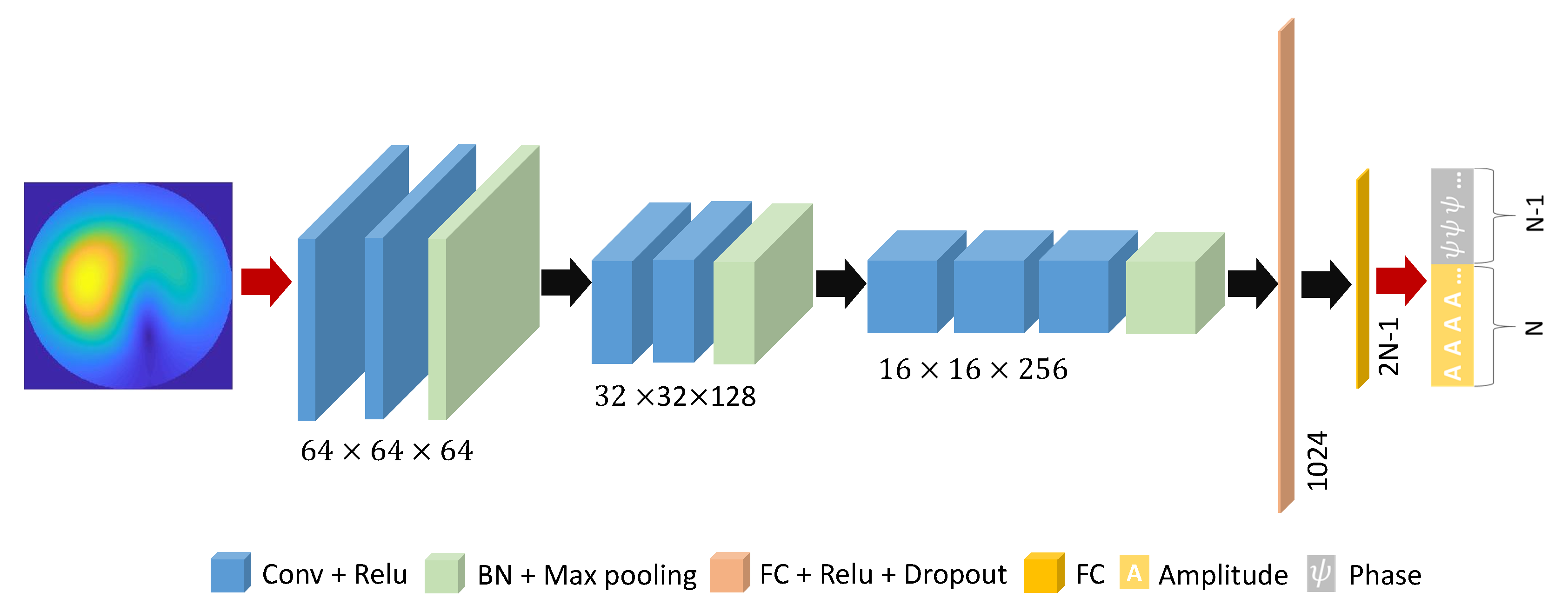
2.2. Deep-Learning-Based Modal Decomposition

DNNs are rapidly developing and have brought prominent impact on various applications, especially computational imaging [26]. The performance of DNNs in image classification and object recognition is well-adapted to understand the complexity of an MMF [27]. This approach does not require consideration of intermodal dispersion, mode coupling, and external perturbations because the network is a data-driven approach. Therefore, a DNN can be used to significantly simplify the evaluation of the output signal of an MMF.
Therefore, an Image-to-vector DNN is designed. The architecture concept was inspired by a convolutional neural network model, which was introduced by Simonyan and Zisserman from the Visual Geometry Group (VGG) at Oxford University [28]. As shown in Figure 1, the DNN is divided into 5 blocks. The first block is composed of two convolutional layers, which perform the same convolutional operation. Several kernel sizes were tested for the respective convolutional layers. It was found that the output of the DNN converges fastest with 3 × 3 kernels. In order to guarantee a proper parameter depth, two convolutional layers with 3 × 3 kernels were used, which have the same receptive field as one convolutional layer with a 5 × 5 kernel [28].
Two convolutional layers use a rectified linear unit (ReLU) [29] activation function. Batch normalization is used to improve the performance of neural network and speed up the convergence [30]. The last layer of the first block is a 2 × 2 max pooling layer with a stride of 2, which reduces the size of the feature map by a factor of 2 and reduces the number of learnable parameters by a factor of 4. The second and third block are similar in structure to the first block, but the number of channels maps doubles, as indicated in Figure 1. The fourth block of the DNN consists of a fully connected layer, which can integrate all the previously collected feature information. The input filter size and the output size of this layer is 8 × 8 × 512 and 1 × 1024 , respectively. In addition, a dropout is used to prevent overfitting. The last block of the DNN is represented by an output layer, which is also a fully connected layer with an input size of 1024 and an output size of 2 N 1 (Equation (2)). In total, the DNN has 12 layers and 18,518,597 learnable parameters.
The input of the DNN is an intensity-only image with the size of 64 × 64 pixels. The output is a 2 N 1 -sized vector, which contains amplitude ρ and phase ϕ information regarding the individual mode weights. It is important to note that there are some hurdles involved in specifying phase information. Ensembles of mode weights with the same amplitude distributions but different phase distributions can provide one and the same intensity image. This is the case if there are different phase values, but the same relative phase difference between the individual modes exists. For this reason, the phase of the fundamental mode was always set to zero and only the relative phase difference between the individual modes was taken into account. This leads to a label vector containing N 1 phase values and solves the problem of ambiguity. In addition, a complex-valued mode field distribution E ̲ MMF provides the same intensity image as its conjugated complex distribution. For this reason, not the real phase difference were used as the label for the datasets, but the cosine Ψ of the phase difference [23]:
Ψ = c o s ( ϕ ) .
With these arrangements, it could be guaranteed that an intensity distribution corresponds to one unique label vector. Further, to predict better results, the values of Ψ were scaled from ( 1 , 1 ) to ( 0 , 1 ) so that the phase labels were in the same range as the amplitude labels.
The precautions taken a priori must also be taken into account if information from the DNN’s predictions is to be evaluated. The amplitude values can be obtained directly from the predicted vector, while the Ψ values should be firstly rescaled from ( 0 , 1 ) to ( 1 , 1 ) , and then the relative phase differences ϕ can be calculated by means of arccos function. At this point however, the ambiguity of the arccos function must be taken into account. For this reason, intensity distributions are first calculated with all possible combinations of the phase values. The final prediction of the DNN is then determined by computing the 2D correlation coefficient Γ between one possible intensity distributions I p and the target distribution I o [31]. Γ is defined as
Γ = R O I ( I p I p ¯ ) ( I o I o ¯ ) R O I ( I p I p ¯ ) 2 R O I ( I o I o ¯ ) 2 ,
where I ¯ indicates the mean value of the respective intensity distribution. The phase vector from which the intensity distribution with the highest correlation coefficient was determined is chosen as the resulting prediction from the DNN.
To evaluate the robustness of a measurement system, the standard deviation σ of multiple measurements is often given. The more robust the measuring system is, the less measured values scatter around a determined mean value. In this work, the respective MD methods are also examined with respect to σ when determining Γ . σ is determined as follows:
σ = 1 N 1 i = 1 N Γ i Γ ¯ 2 ,
where Γ ¯ is the mean correlation value.

2.3. Specified Mode Combinations (SMC) Data Design for the Training Process

For the training process of the network, data must be generated from which the network can extract characteristic properties about the problem at hand. For the presented problem, one ensemble of the training dataset consists of an intensity distribution and the label vector with the corresponding mode weights. Each change of an element of the mode weights also leads to a change in the intensity distribution. Therefore, the aim is to make the training data as representative as possible. A trivial possibility is to specify a certain number of random combinations of mode weights and to determine random intensity distributions from them. With this procedure however, the required size of the dataset will become immensely large with increasing complexity or increasing number of modes in order to be able to make an accurate prediction. For this reason, a new approach was chosen in order to ensure the most accurate prediction of the network as well as a manageable size of the training dataset. For this purpose, all combinations of mode field distributions are synthetically created and varied with two predefined step widths—one for amplitude s a m p and one for the phase s p h a s e of the respective mode. This means that the total amount of generated training data is dependent on both step sizes. The approximate amount of data M can be computed by
M 1 s a m p + 1 N · 1 s p h a s e + 1 N 1 .
Additionally, duplicate ensembles of the dataset are eliminated, which is why the final value of M is reduced. Eventually, a defined vector with N magnitude and N 1 relative phase distances is generated for each ensemble of the training dataset. In addition, care is taken to ensure that the Euclidean standard of the amplitude weights remains constant at 1, which is why the amplitude values are normalized. Finally, both the amplitude and phase values are additive, superimposed with white noise, the level of which is as large as half the respective step size. This procedure is performed in order to generate amplitude and phase distributions that are as realistic as possible. The resulting label vector for the training dataset is then generated by computing the cosine of the phase value (Equation (5)). The method of training data design is referred to in the following as Specified Mode Combinations (SMC).

3. Results

In the following, the performance of the introduced DNN and the SMC training data design will be presented based on both simulation and experimental environments. For this purpose, a step-index MMF with a core radius of 4 μ m, NA = 0.1 , and λ = 932 nm wavelength is assumed. Since LP modes are also valid for parabolic refractive index profiles, the DNN could theoretically be used for graded-index fibers.
The considered fiber can guide N = 3 LP modes. Such fibers are known as few-mode fibers (FMF). The presented method can be potentially applied to MMFs, but is tested in an FMF realizing fundamental investigations.
The SMC dataset is generated with the step sizes s a m p = 0.125 and s p h a s e = 0.1 , resulting in 59,018 64 × 64 -sized intensity distributions and corresponding label vectors with 5 entries. The scheme of the SMC procedure is shown in Figure 2.

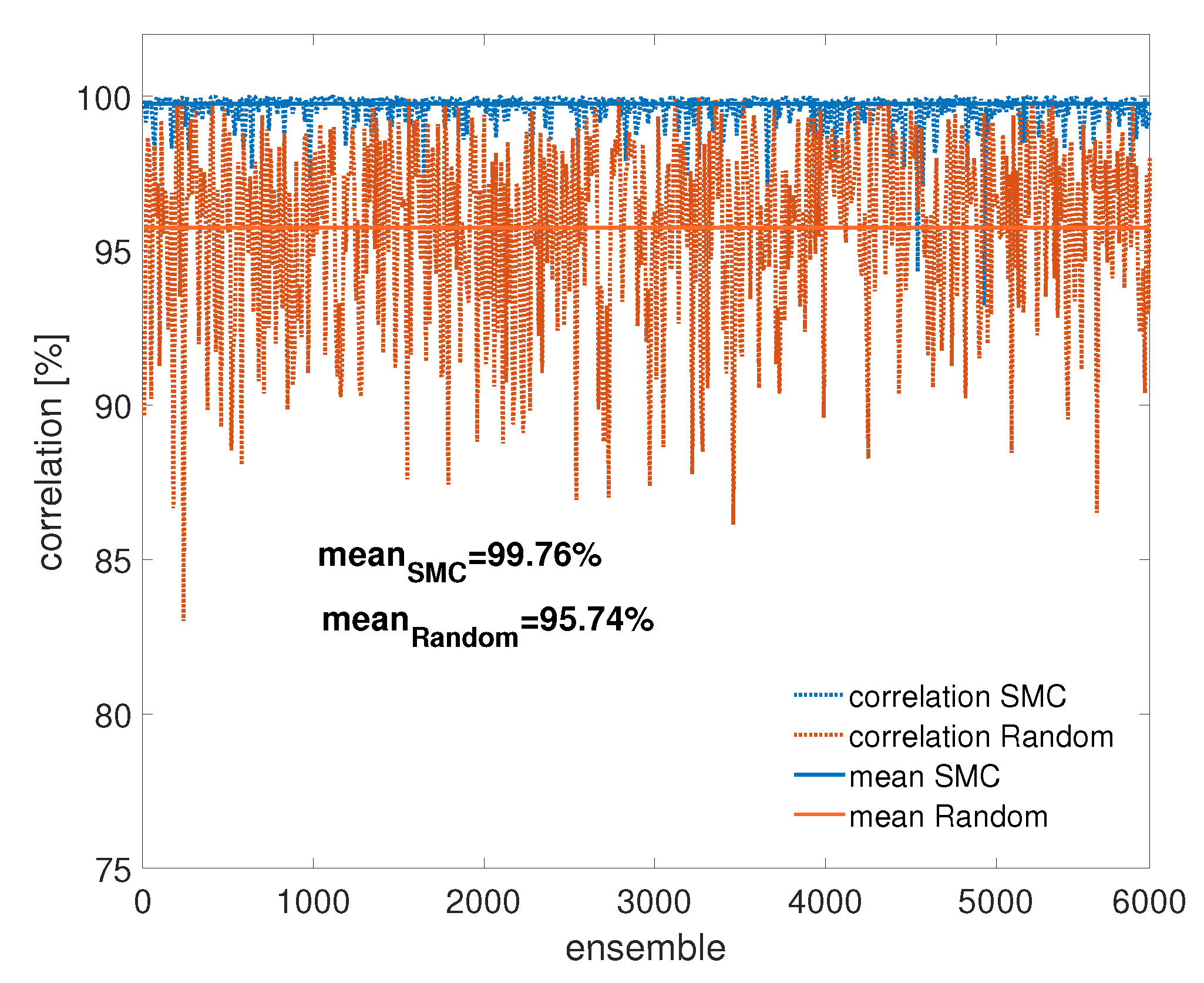
3.1. Performance of the SMC Data Design

First, the dataset is randomly split into a training dataset, a validation dataset, and a test dataset, with a ratio of 8:1:1. During the training process, the minibatch size is set to 128. The learning rate is set to 0.001 initially and reduced by a factor of 2 every 20 epochs. The loss function is defined as the mean-square-error (MSE) between the prediction p and the label l vector:
M S E = i = 1 2 N 1 ( l i p i ) 2 2 N 1 .
Adam [32] is chosen as the optimization algorithm of the training progress. After 73,800 iterations, the DNN eventually converged. Afterwards, the trained DNN is tested with 5902 images. The relative errors (the maximum of the amplitude of the weights is 1) of the mode weight prediction are determined as follows:
Δ ρ p = | ρ p ρ o | , and Δ ϕ p = | ϕ p ϕ o | 2 π ,
where p indicates a predicted value and o indicates an original value. The predicted weights are further used to generate a predicted intensity distribution, which is then correlated with the respective original distribution (Equation (6)).
For a quantitative evaluation of the performance of the presented SMC training data design, we have trained the same network under the same conditions with purely random mode combinations. In Table 1, the results of both training methods are shown.
It was found that the mean relative deviation when mode weights are predicted using the SMC data design is 1.8 % for phase and 0.98 % for amplitude, whereas the mean relative error of using random mode combinations for training the DNN is 7.32 % and 6.48 % , respectively, for phase and amplitude. Based on the predicted weights, the intensity distributions of the mode fields are again computed and correlated with the original intensity distributions (Equation (6)). Using the SMC dataset, a mean correlation coefficient of 99.61 % could be achieved, whereas the mean correlation coefficient obtained by using random mode combinations has a value of 95.74 % . The respective correlation coefficients are shown in Figure 3. Using the SMC training data design, the obtained correlation results scatter around the mean correlation coefficient with σ = 0.57 % (Equation (7)). Using random mode combinations for the training data, the standard deviation increases significantly to 3.24 % .

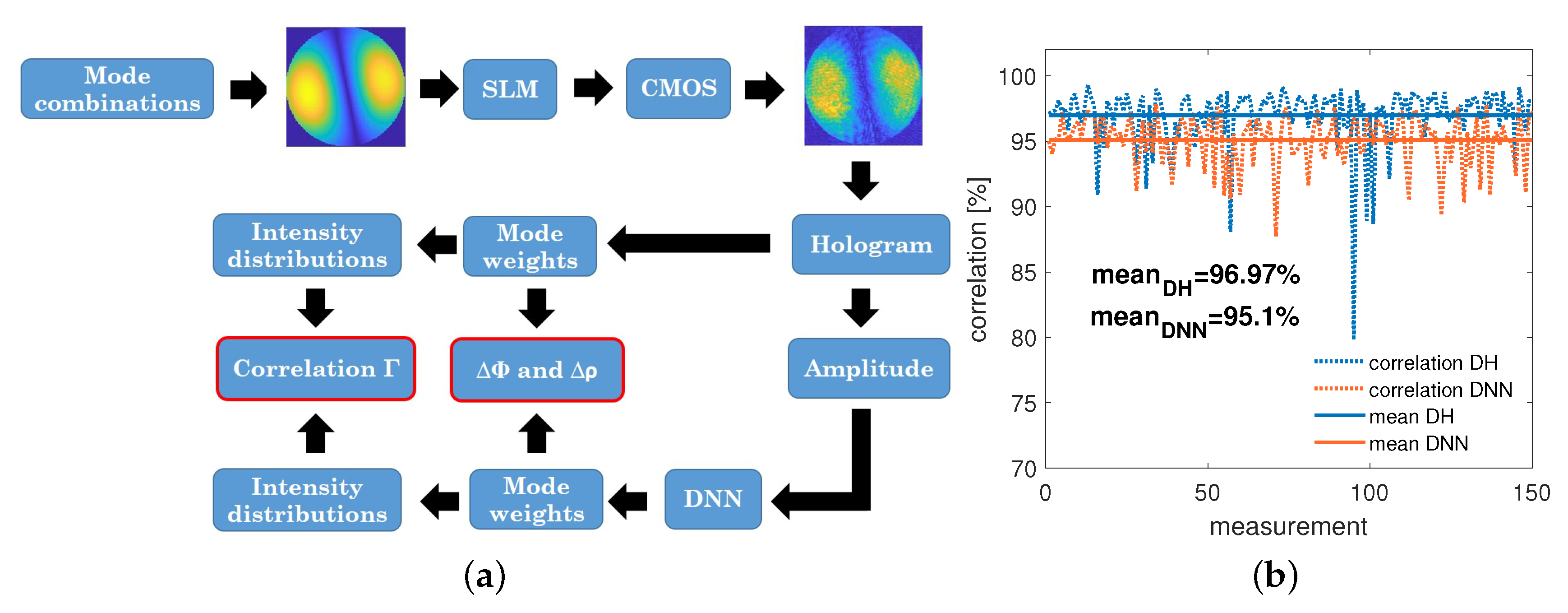
3.2. Performance of the DNN Using Experimental Data

It has to be shown that with known FMF parameters it is possible to train a DNN in such a way that a complex-valued MD can be performed based on pure intensity images in an experimental environment. Therefore, random mode combinations can be created assuming the same FMF parameters used in the previous section. The respective light fields are shaped subsequently with the help of a Spatial Light Modulator (SLM) using superpixels and imaged with a camera.
In Figure 4, the optical setup used to capture the individual mode field distributions purely intensity-based as well as holographically, is demonstrated. As it has already been introduced in prior work [19], the system is originally intended for selective mode excitation with an MMF. A single-mode fiber (SMF) is used for spatial filtering of a laser beam to ensure the best beam profile for the experiments. The beam is then collimated (CP) and expanded using a beam expander (BE). Since the SLM is only suitable for linear polarization directions, a polarizing beam splitter (PBS) and a half-wave plate (HWP) are used to filter the required polarization direction. Lens L1 is performing an FFT with the light field which is reflected off the surface of the SLM. Since a diffraction grating is added to the phase-mask which is displayed on the SLM, the modulated light field is separated spatially into the respective diffraction orders. The fully modulated light signal is located in the higher diffraction orders, whereas the nonmodulated background is located in the 0th order. In the Fourier domain, the 1st diffraction order is filtered spatially with IB1 to let the individual superpixels mix with each other and inverse Fourier transformed with L2 afterwards. The generated light field is then imaged onto a CMOS camera propagating through 2 telescopes (L3–L4 and L4–L5). The captured images are cut out and fed into the network, to predict the chosen mode weights. In addition, it is possible to record the light field distributions for the second experiment series holographically. For this purpose, the laser beam used in the optical setup is additionally split into a reference beam using BS1. For this reason, a beam cleanup is performed for the reference beam using two lenses L4 and L5, as well as a pinhole IB2, in order to generate a beam profile that is as pure as possible. The recorded hologram is then used to determine the individual complex weights according to Equation (4). If purely intensity-based images should be captured, the reference beam has to be blocked.
In order to compare the quality of the DNN-based MD with the holography-based MD (Equation (4)), 150 different and random mode field distributions are captured. To ensure a fair comparison between the DNN and the holographic method, the amplitude distributions from the holographic measurement were used as input for the DNN. The respective mean relative errors (Equation (10)) are shown in Table 2.
Using DH, a mean relative error of the phase and amplitude determination of the mode weights of 4.20 % and 3.32 % could be achieved, respectively. The DNN prediction of the mode weights using the SMC dataset is afflicted with a mean relative error of 9.45 % and 6.02 % for phase and amplitude, respectively, or 11.03 % and 9.56 % using random mode combinations for training the DNN. As it is shown in Figure 5a, based on measured, respectively predicted weights, the intensity distributions of the mode fields are computed and correlated with the original intensity distributions (Equation (6)). Using DH, a mean correlation coefficient of 96.97 % with σ = 2.26 % could be achieved, whereas the mean correlation obtained by using the DNN, which was trained with the SMC dataset, has a value of 95.10 % with σ = 1.90 % . Using a DNN, which was trained with random mode combinations, achieves worse results. The mean correlation coefficient is 92.24 % with σ = 3.17 % . The respective correlation coefficients of both DH and the DNN trained with the SMC dataset are shown in Figure 5b.
It can be seen that the achieved correlation coefficients in the experiment are reduced with respect to the simulation results. This can be explained with imperfections of the optical system, including the SLM, optical components, and the camera. A thorough description of the individual error sources is given in the discussion.

4. Discussion

First, the results using synthetic data for mode weight prediction show that with the SMC training data design, a significant improvement of a complex-valued MD can be achieved. The DNN was trained with a dataset containing ≈ 60,000 ensembles using predefined step sizes. With smaller step sizes, the amount of data would increase, which would lead to an improvement of the performance. This would also lead to a longer training phase of the DNN. The chosen step sizes resulted from a trade-off between performance and computational load. For the MD, an FMF was assumed, which can guide 3 modes. Increasing the number of modes and, thus, the complexity of the problem would also have an effect on the result. In this case, the DNN had to be trained with more data or had to be designed more deep to achieve equivalent results.
Second, the DNN-based MD was applied to an experimental environment using the same synthetic SMC dataset. The aim is to create a measurement system, which can evaluate the mode weights in phase and amplitude with intensity-only measurements. An SLM was used to generate random mode combinations of the 3 modes the assumed FMF can guide. The light field distributions are then imaged to a CMOS camera, where holograms are captured and evaluated using the angular spectrum method. To ensure a fair comparison between the DNN and the DH method, the amplitude distributions from the holographic measurement were used as input for the DNN. Both the DNN and DH are utilized to run a complex MD. In the determination of the individual mode weights, it could be shown that the phase determination has a mean deviation of 4.20 % using DH and 9.45 % using the SMC-based DNN. The amplitude determination could be carried out with DH with a mean deviation of 3.32 % and with the SMC-based DNN with a mean deviation of 6.02 % . Although the phase determination with DH is better by a factor of 2, similar correlation values can be achieved with the original images. With DH, a mean correlation coefficient of 96.91 % and 95.10 % with the SMC-based DNN could be achieved. These results clearly show that a DNN shows equivalent results to an established measurement technique like DH. Although neither a phase measurement was carried out nor were sources of error of optical components learned in the training process, the results are comparable. These relationships clearly emphasize the potential of DNNs. Nevertheless, it can be observed that the results with measured data are significantly below the results using simulation data. This is mainly due to the fact that the optical system for collecting the measured data is not perfect. One source of error is the simultaneous amplitude and phase modulation with the phase-only SLM using superpixels. Only a discrete number of pixels can be used for the individual superpixels. An optimum of 6 × 6 pixels was found for this. Additionally, SLMs are known for their phase flicker property [33] and have a modulation efficiency < 1, which leads to unwanted background light and errors. Therefore, the superpixel phase-mask is superimposed with a diffraction grating. The actual modulated light is spatially separated in the Fourier plane of L1 (1st diffraction order) and can therefore be filtered with a pinhole. Further, imaging errors, aberrations of optical components, and quantization noise are additional possible error sources in the optical setup. These sources of error are significant for both DH and the DNN. It is therefore important to find out how these error terms can be compensated in the future when using DNN with the help of suitable training data. However, it can already be stated at this point that the DNN reacts extremely robustly to experimental error sources which have not been learned in advance during the training process.

5. Conclusions

A measurement system based on a deep neural network was developed that can perform complex mode decomposition. For this purpose, the training data were created synthetically using images with only intensity of certain mode combinations. The introduced design concept leads to a significant improvement in mode decomposition in terms of accuracy and precision compared to conventional training data based on random mode combinations ( 99.61 % vs. 95.74 % correlation). The same network was tested with experimental data. Although neither a phase measurement was carried out, nor sources of error of optical components in the training process determined, the results of the mode decomposition are comparable to those of a proven measurement technique such as digital holography. The results underline the potential of neural networks for modern, intelligent measurement systems for industrial applications.

Author Contributions

J.W.C. and N.K. contributed to the idea of using complex mode decomposition methods to measure the transmission matrix of multimode fibers. S.R. is responsible for the ideas of using deep learning for mode decomposition and the SMC training data design. S.R. designed, built, programmed, and characterized the setup for generating experimental data. Q.Z. designed and programmed the DNN. S.R. and Q.Z. wrote the article. J.W.C. supervised the whole research work. N.K. and J.W.C. revised the article. All authors have read and agreed to the published version of the manuscript.

Funding

This research was funded by Deutsche Forschungsgemeinschaft (DFG) grant number (CZ 55/42-1).

Acknowledgments

The authors are grateful to Robert Kuschmierz and Richard Nauber for helpful discussions and extensive comments on earlier versions of the paper.

Conflicts of Interest

The authors declare no conflict of interest.

References

  1. Čižmár, T.; Dholakia, K. Exploiting multimode waveguides for pure fibre-based imaging. Nat. Commun. 2012, 3, 1027. [Google Scholar] [CrossRef] [PubMed] [Green Version]
  2. Kuschmierz, R.; Scharf, E.; Koukourakis, N.; Czarske, J.W. Self-calibration of lensless holographic endoscope using programmable guide stars. Opt. Lett. 2018, 43, 2997–3000. [Google Scholar] [CrossRef] [PubMed]
  3. Ryf, R.; Randel, S.; Gnauck, A.H.; Bolle, C.; Sierra, A.; Mumtaz, S.; Esmaeelpour, M.; Burrows, E.C.; Essiambre, R.J.; Winzer, P.J.; et al. Mode-Division Multiplexing Over 96 km of Few-Mode Fiber Using Coherent 6×6 MIMO Processing. J. Light. Technol. 2011, 30, 521–531. [Google Scholar] [CrossRef]
  4. Garito, A.; Wang, J.; Gao, R. Effects of random perturbations in plastic optical fibers. Science 1998, 281, 962–967. [Google Scholar] [CrossRef] [PubMed]
  5. Gover, A.; Lee, C.; Yariv, A. Direct transmission of pictorial information in multimode optical fibers. JOSA 1976, 66, 306–311. [Google Scholar] [CrossRef] [Green Version]
  6. Vellekoop, I.M.; Mosk, A. Focusing coherent light through opaque strongly scattering media. Opt. Lett. 2007, 32, 2309–2311. [Google Scholar] [CrossRef]
  7. Mahalati, R.N.; Askarov, D.; Wilde, J.P.; Kahn, J.M. Adaptive control of input field to achieve desired output intensity profile in multimode fiber with random mode coupling. Opt. Express 2012, 20, 14321–14337. [Google Scholar] [CrossRef] [Green Version]
  8. Čižmár, T.; Dholakia, K. Shaping the light transmission through a multimode optical fibre: Complex transformation analysis and applications in biophotonics. Opt. Express 2011, 19, 18871–18884. [Google Scholar] [CrossRef] [Green Version]
  9. Cui, M.; Yang, C. Implementation of a digital optical phase conjugation system and its application to study the robustness of turbidity suppression by phase conjugation. Opt. Express 2010, 18, 3444–3455. [Google Scholar] [CrossRef] [Green Version]
  10. Papadopoulos, I.N.; Farahi, S.; Moser, C.; Psaltis, D. Focusing and scanning light through a multimode optical fiber using digital phase conjugation. Opt. Express 2012, 20, 10583–10590. [Google Scholar] [CrossRef]
  11. Czarske, J.W.; Haufe, D.; Koukourakis, N.; Büttner, L. Transmission of independent signals through a multimode fiber using digital optical phase conjugation. Opt. Express 2016, 24, 15128–15136. [Google Scholar] [CrossRef] [PubMed]
  12. Bianchi, S.; Di Leonardo, R. A multi-mode fiber probe for holographic micromanipulation and microscopy. Lab Chip 2012, 12, 635–639. [Google Scholar] [CrossRef] [PubMed]
  13. Plöschner, M.; Tyc, T.; Čižmár, T. Seeing through chaos in multimode fibres. Nat. Photonics 2015, 9, 529–535. [Google Scholar] [CrossRef]
  14. Carpenter, J.; Thomsen, B.C.; Wilkinson, T.D. Degenerate mode-group division multiplexing. J. Light. Technol. 2012, 30, 3946–3952. [Google Scholar] [CrossRef]
  15. Loterie, D.; Farahi, S.; Papadopoulos, I.; Goy, A.; Psaltis, D.; Moser, C. Digital confocal microscopy through a multimode fiber. Opt. Express 2015, 23, 23845–23858. [Google Scholar] [CrossRef] [PubMed] [Green Version]
  16. Caravaca-Aguirre, A.M.; Niv, E.; Conkey, D.B.; Piestun, R. Real-time resilient focusing through a bending multimode fiber. Opt. Express 2013, 21, 12881–12887. [Google Scholar] [CrossRef] [PubMed] [Green Version]
  17. Nicholson, J.; Yablon, A.D.; Ramachandran, S.; Ghalmi, S. Spatially and spectrally resolved imaging of modal content in large-mode-area fibers. Opt. Express 2008, 16, 7233–7243. [Google Scholar] [CrossRef]
  18. Rothe, S.; Koukourakis, N.; Radner, H.; Lonnstrom, A.; Jorswieck, E.; Czarske, J.W. Physical Layer Security in Multimode Fiber Optical Networks. Sci. Rep. 2020, 10, 2740. [Google Scholar] [CrossRef]
  19. Rothe, S.; Radner, H.; Koukourakis, N.; Czarske, J. Transmission Matrix Measurement of Multimode Optical Fibers by Mode-Selective Excitation Using One Spatial Light Modulator. Appl. Sci. 2019, 9, 195. [Google Scholar] [CrossRef] [Green Version]
  20. Mir, M.; Bhaduri, B.; Wang, R.; Zhu, R.; Popescu, G. Quantitative phase imaging. Prog. Opt. 2012, 57, 133–217. [Google Scholar]
  21. Loterie, D.; Farahi, S.; Psaltis, D.; Moser, C. Complex pattern projection through a multimode fiber. In Adaptive Optics and Wavefront Control for Biological Systems; International Society for Optics and Photonics: Bellingham, WA, USA, 2015; Volume 9335, p. 93350I. [Google Scholar]
  22. Bhaduri, B.; Edwards, C.; Pham, H.; Zhou, R.; Nguyen, T.H.; Goddard, L.L.; Popescu, G. Diffraction phase microscopy: Principles and applications in materials and life sciences. Adv. Opt. Photonics 2014, 6, 57–119. [Google Scholar] [CrossRef]
  23. An, Y.; Huang, L.; Li, J.; Leng, J.; Yang, L.; Zhou, P. Learning to decompose the modes in few-mode fibers with deep convolutional neural network. Opt. Express 2019, 27, 10127–10137. [Google Scholar] [CrossRef] [PubMed]
  24. Gloge, D. Weakly guiding fibers. Appl. Opt. 1971, 10, 2252–2258. [Google Scholar] [CrossRef] [PubMed] [Green Version]
  25. Koukourakis, N.; Abdelwahab, T.; Li, M.Y.; Höpfner, H.; Lai, Y.W.; Darakis, E.; Brenner, C.; Gerhardt, N.C.; Hofmann, M.R. Photorefractive two-wave mixing for image amplification in digital holography. Opt. Express 2011, 19, 22004–22023. [Google Scholar] [CrossRef]
  26. Barbastathis, G.; Ozcan, A.; Situ, G. On the use of deep learning for computational imaging. Optica 2019, 6, 921–943. [Google Scholar] [CrossRef]
  27. Borhani, N.; Kakkava, E.; Moser, C.; Psaltis, D. Learning to see through multimode fibers. Optica 2018, 5, 960–966. [Google Scholar] [CrossRef]
  28. Simonyan, K.; Zisserman, A. Very deep convolutional networks for large-scale image recognition. arXiv 2014, arXiv:1409.1556. [Google Scholar]
  29. Glorot, X.; Bordes, A.; Bengio, Y. Deep sparse rectifier neural networks. In Proceedings of the Fourteenth International Conference on Artificial Intelligence and Statistics, Fort Lauderdale, FL, USA, 11–13 April 2011; pp. 315–323. [Google Scholar]
  30. Ioffe, S.; Szegedy, C. Batch normalization: Accelerating deep network training by reducing internal covariate shift. arXiv 2015, arXiv:1502.03167. [Google Scholar]
  31. Brüning, R.; Gelszinnis, P.; Schulze, C.; Flamm, D.; Duparré, M. Comparative analysis of numerical methods for the mode analysis of laser beams. Appl. Opt. 2013, 52, 7769–7777. [Google Scholar] [CrossRef]
  32. Kingma, D.P.; Ba, J. Adam: A method for stochastic optimization. arXiv 2014, arXiv:1412.6980. [Google Scholar]
  33. García-Márquez, J.; López, V.; González-Vega, A.; Noé, E. Flicker minimization in an LCoS spatial light modulator. Opt. Express 2012, 20, 8431–8441. [Google Scholar] [CrossRef] [PubMed]
Figure 1. Architecture of the deep neural network (DNN) used to run a mode decomposition (MD).
Applsci 10 01367 g001
Figure 2. With a selected FMF and known parameters, the modes, which can be guided through the waveguide, can be calculated. Specified mode combinations are then generated, resulting in ensembles of a label vector and a corresponding intensity distribution.
Applsci 10 01367 g002
Figure 3. Correlation coefficients using Specified Mode Combinations (SMC), respectively, random mode combinations for training the DNN. For better readability, an exemplary selection of the ≈6000 results are depicted in the figure.
Applsci 10 01367 g003
Figure 4. Optical setup, which is used to generate random mode field distributions using an SLM. The generated light fields can be measured either purely intensity-based or holographically.
Applsci 10 01367 g004
Figure 5. (a) Illustration of the scheme for data acquisition. (b) Correlation coefficients using DH and the prediction of a DNN, respectively.
Applsci 10 01367 g005
Table 1. Mean relative errors for the mode weight prediction using both Specified Mode Combinations (SMC) and random mode combinations for training the DNN.
Δ ϕ s ¯ Δ ρ s ¯ Γ ¯ σ
SMC 1.80 % 0.98 % 99.61 % 0.57 %
Random 7.32 % 6.48 % 95.74 % 3.24 %
Table 2. Mean relative errors of the mode weight determination using Digital Holography (DH) or a DNN.
Δ ϕ s ¯ Δ ρ s ¯ Γ ¯ σ
DH 4.20 % 3.32 % 96.97 % 2.26 %
DNN SMC 9.45 % 6.02 % 95.10 % 1.90 %
DNN random 11.03 % 9.56 % 92.24 % 3.17 %

