A Practical Method for Controlling the Asymmetric Mode of Atmospheric Dielectric Barrier Discharges

Abstract

Atmospheric pressure dielectric barrier discharges (DBDs) have been applied in a very broad range of industries due to their outstanding advantages. However, different discharge modes can influence the stability of atmospheric DBDs, such as the density and composition of active species in discharge plasmas, thereby impacting the effect of related applications. It is necessary and valuable to investigate the control of nonlinear modes both in theoretical and practical aspects. In this paper, we propose a practical, state-controlling method to switch the discharge mode from asymmetry to symmetry through changing frequencies of the applied voltage. The simulation results show that changing frequencies can effectively alter the seed electron level at the beginning of the breakdown and then influence the subsequent discharge mode. The higher controlling frequency is recommended since it can limit the dissipative process of residual electrons and is in favor of the formation of symmetric discharge in the after-controlling section. Under our simulation conditions, the discharges with an initial driving frequency of 14 kHz can always be converted to the symmetric period-one mode when the controlling frequency is beyond 30 kHz.

1. Introduction

Atmospheric dielectric barrier discharges (DBDs), due to their advantages in producing low-temperature plasmas without a precise vacuum chamber, have been widely used in a lot of industrial applications such as surface modification, energy transformation, biomedical sterilization, and pollution abatement [1,2,3,4,5]. Such pervasive applications have already made DBDs a prospective and an active research topic for many years.

Being a nonequilibrium dissipative system, DBDs can exhibit an abundance of nonlinear characteristics or phenomena which are extremely sensitive to the operational environment and controlled parameters [6]. Typically, it is well known that in most cases atmospheric DBDs appear as a symmetric period-one discharge (henceforth called SP1), that is, the shape and amplitude of positive and negative current pulses are basically identical and repeat every one applied voltage cycle [7]. However, under certain conditions, a lot of simulation and experimental research has reported that DBDs can also work in various nonlinear modes such as asymmetric period-one (henceforth called AP1), multi-period, quasi-period and chaos through different evolution routes [8,9,10,11]. Since different discharge modes can influence the stability of DBDs in terms of the density and composition of active species in discharge plasmas and then impact their efficacy in related applications [12,13], the investigation on the control of nonlinear modes is valuable and imperative both in theoretical and practical aspects. It is worth noting that before bifurcating into other nonlinear modes from SP1, the discharge always first transforms into the asymmetric mode as a transition phase [14]. Therefore, investigating the mechanisms related to the asymmetric discharge mode could serve as a stepping-stone for the interpretation of other, more complex nonlinear behaviors in DBDs and deserve more attention.

The initiation mechanism regarding the SP1-AP1 transition was first reported by Golubovskii et al. in 2003 [15]. Through the numerical simulation of a homogeneous DBD, they observed the SP1-AP1 transition at both lower and higher concentrations of nitrogen impurities, and they concluded that such a mode transition is contributed by the residual quasi-neutral (plasma) region. Our group has also made some effort on this aspect. According to our previous works, the SP1-AP1 transition in shorter gaps might be attributed to the discordance of the evolutionary paces between electrons and ions [16], while, in longer gaps, the rise in seed electron level induced by the electron backflow is the main reason for the generation of AP1 discharge [17], and the traditional explanations such as “residual positive column” [7] or “instantaneous anode” [18] in essence are special forms of the “electron backflow region”. Furthermore, we also proposed a preliminary state-controlling method which can adjust the discharge mode from AP1 to SP1 by applying a first-peak-leveled driving voltage from the beginning of the discharge [19].

Despite all those discoveries, there are still many obstacles that hinder the application of mode controlling in practical industrial applications. For example, the most favored condition in practical applications is that the discharge mode needs to switch to SP1 mode right after asymmetric discharges occur, which was not achieved in previous studies. In addition, the existing method needs to compute the initial moment of the flat-top stage, which is inconvenient for practical devices. Note that the frequency of the applied voltage can also influence the distribution of seed electrons as the amplitude of the voltage does, and changing the frequency of the power supply is much easier to implement for practical power supply devices. Therefore, in this paper, we try to use a more practical method to switch AP1 discharge into SP1 discharge by changing the driving frequency. More specifically, we first adjust the original driving frequency f_d to a different controlling frequency f_c for a certain period of time, right after the establishment of AP1 discharge. Once the discharge stabilizes under f_c, the driving frequency will be changed back to the initial value (i.e., f_d). The rest of this paper is organized as follows: Section 2 briefly introduces the one-dimensional fluid model and its qualitative validation; the numerical regulating example and its underneath mechanism are shown in Section 3; the key conclusions are drawn in Section 4; Appendix A presents the chemical scheme used in our simulation.

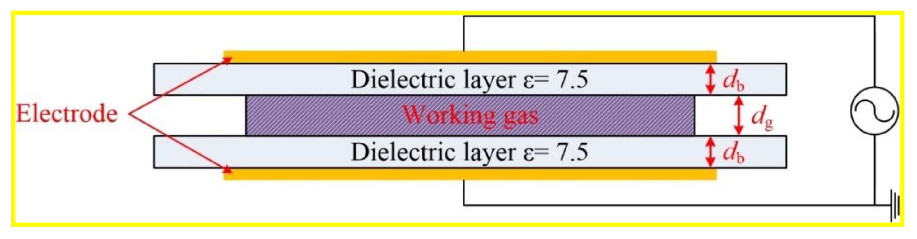
2. Model Description

As shown in Figure 1, the atmospheric DBD considered in the simulation is generated in a gap filled with pure helium between two parallel-plate electrodes, both covered by a thin dielectric layer with a relative permittivity of 7.5, corresponding to the value of mica glass. The upper electrode is connected to a sinusoidal voltage with an amplitude V_am of 2 kV, whereas the lower one is grounded. The width of the gas gap d_g is fixed to 4.4 mm and the dielectric layer thickness d_b is 1 mm. Note that the gap width is not very large (<5 mm) and much shorter compared with the radius of electrodes (≈56.4 mm) [20]; in this case, the radially homogeneous assumption should be reasonable and accepted. On this basis, a one-dimensional fluid model is appropriate to simulate the discharge process, which has also been successfully applied to investigate the nonlinear phenomena in [6,21,22].

In the 1-D fluid model, electron properties, including the electron density and energy density, are governed by the Boltzmann equation under drift-diffusion approximation [23,24,25], as given by Equations (1)–(4); Equations (5) and (6) are multi-component transport equations [26,27] determining the flux of heavy species. Besides, in order to determine the electric field distribution, Poisson’s equation is firmly coupled.

$$\frac{\partial n_{\mathrm{e}}}{\partial t}+\nabla \cdot {\mathit{\Gamma }}_{\mathrm{e}}=S_{\mathrm{e}}$$

(1)

$$\frac{\partial n_{\mathsf{\epsilon }}}{\partial t}+\nabla \cdot {\mathit{\Gamma }}_{\mathsf{\epsilon }}+E{\mathit{\Gamma }}_{\mathrm{e}}=S_{\mathrm{en}}$$

(2)

$${\mathit{\Gamma }}_{\mathrm{e}}=-{\mu }_{\mathrm{e}}{n}_{\mathrm{e}}\mathit{E}-D_{\mathrm{e}}\nabla \cdot n_{\mathrm{e}}$$

(3)

$${\mathit{\Gamma }}_{\mathsf{\epsilon }}=-\frac{5}{3}{\mu }_{\mathrm{e}}{n}_{\mathsf{\epsilon }}\mathit{E}-\frac{5}{3}{D}_{\mathrm{e}}\nabla \cdot n_{\mathsf{\epsilon }}$$

(4)

$$\rho \frac{\partial {\omega }_k}{\partial t}=\nabla \cdot J_k+S_k$$

(5)

$$J_k=\rho {\omega }_k(D_k\frac{\nabla {\omega }_k}{{\omega }_k}+D_k\frac{\nabla M_n}{M_n}-z_k{\mu }_{k}E)$$

(6)

Here, n_e, n_ε, Γ_e, and Γ_ε respectively denote the electron number density, electron energy, total electron flux, and electron energy flux; J_k is the flux vector for heavy species k, and its mass fraction and charge number are ω_k and z_k, respectively; S_e, S_en, and S_k respectively represent the source terms describing the net changing rate of electron density, electron energy loss/gain, and the source term for heavy species k; the electron mobility μ_e is solved by Bolsig⁺ with the cross-section data from IST-Lisbon Database [28,29,30], then the electron diffusion coefficient D_e can be obtained through Einstein’s relation [29]; the mobility and diffusion coefficient for heavy species k, i.e., μ_k and D_k, are referenced from [25]; E is the electric field intensity; the mixture properties ρ and M_n stand for the density of mixture and its mean molar mass.

The “wall” boundary applied at the surfaces sandwiched between plasma and dielectrics provides two sets of equations, describing the particle flux (Equations (7)–(9)) and the charge accumulation (Equations (10) and (11)), respectively.

$$n\cdot {\mathit{\Gamma }}_{\mathrm{e}}=\frac{1}{2}{v}_{\mathrm{e},\mathrm{th}}{n}_{\mathrm{e}}-{\alpha }_{\mathrm{s}}{n}_{\mathrm{e}}{\mu }_{\mathrm{e}}\mathit{E}\cdot n-{\displaystyle \sum _i{\gamma }_i({\mathit{\Gamma }}_i\cdot n)}$$

(7)

$$\mathbf{n}\cdot {\mathit{\Gamma }}_{\mathsf{\epsilon }}=\frac{5}{6}{v}_{\mathrm{e},\mathrm{th}}{n}_{\mathsf{\epsilon }}-{\alpha }_{\mathrm{s}}{n}_{\mathsf{\epsilon }}{\mu }_{\mathsf{\epsilon }}\mathit{E}\cdot \mathbf{n}-{\displaystyle \sum _i{\gamma }_i\overline{{\epsilon }_i}({\mathit{\Gamma }}_i\cdot \mathbf{n})}$$

(8)

$$\mathbf{n}\cdot {\mathit{\Gamma }}_k=M_k{R}_{\mathrm{surf},k}+{\alpha }_{\mathrm{s}}{M}_k{c}_k{\mu }_{k,m}{z}_k\mathit{E}\cdot \mathbf{n}$$

(9)

$$\frac{\mathrm{d}{\sigma }_{\mathrm{s}}}{\mathrm{d}t}={\mathit{J}}_{\mathrm{e}}\cdot \mathbf{n}+{\mathit{J}}_i\cdot \mathbf{n}$$

(10)

$${\sigma }_{\mathrm{s}}=({\mathit{D}}_2-{\mathit{D}}_1)\cdot \mathbf{n}$$

(11)

Here, n is the unit normal vector towards the surface; both Γ_k and Γ_i stand for the boundary flux of heavy species but the latter only denotes the term for ions; v_e,th is the thermal velocity; M_k represents the molar weight; R_surf,k is the surface reaction rate; γ_i is the emission coefficient of the secondary electron cited from [25] and $\overline{{{\displaystyle \epsilon }}_i}$ is its mean energy; σ_s represents the surface charge density on the wall, and J_e and J_i respectively denote the electron density and the ion density there; D₁ and D₂ are the electric displacement vectors on both sides of the interface; α_s is a switching function as given below.

$${\alpha }_{\mathrm{s}}=\{\begin{array}{l}1,\mathrm{sgn}(q)\mathit{E}\cdot \mathbf{n}>0\\ 0,\mathrm{sgn}(q)\mathit{E}\cdot \mathbf{n}\le 0\end{array}$$

(12)

Here, q represents the signed charge.

For chemical kinetics, we reused ones from our previous work [19]. To be specific, the model sustains itself under the pressure of 760 Torr and temperature of 300 K, and it considers six particles (i.e., e (electron), He, He*, He₂*, He⁺ and He₂⁺) and 27 reactions which are listed in

Table A1. Chemical reactions considered in the model.

Index	Reaction	Rate Coefficient	Reference
R1	$\mathrm{e}+\mathrm{He}=>\mathrm{e}+\mathrm{He}$	$f\left(T_{\mathrm{e}}\right)$	[30]
R2	$\mathrm{e}+\mathrm{He}=>\mathrm{e}+{\mathrm{He}}^{*}$	$f\left(T_{\mathrm{e}}\right)$	[30]
R3	$\mathrm{e}+\mathrm{He}=>2\mathrm{e}+{\mathrm{He}}^{+}$	$f\left(T_{\mathrm{e}}\right)$	[30]
R4	$\mathrm{e}+{\mathrm{He}}^{*}=>2\mathrm{e}+{\mathrm{He}}^{+}$	$1.28\times {10}^{-7}\times T_{\mathrm{e}}^{0.6}\times \exp \left(-4.78/T_{\mathrm{e}}\right)$	[31]
R5	$\mathrm{e}+{\mathrm{He}}^{*}=>\mathrm{e}+\mathrm{He}$	$2.9\times {10}^{-9}$	[31]
R6	$\mathrm{e}+{\mathrm{He}}_2^{*}=>\mathrm{e}+2\mathrm{He}$	$3.8\times {10}^{-9}$	[31]
R7	$2\mathrm{e}+{\mathrm{He}}^{+}=>\mathrm{e}+{\mathrm{He}}^{*}$	$5.82\times {10}^{-20}\times {\left(T_{\mathrm{e}}/0.026\right)}^{-4.4}$	[31]
R8	$2\mathrm{e}+{\mathrm{He}}_2^{+}=>{\mathrm{He}}^{*}+\mathrm{He}+\mathrm{e}$	$2.8\times {10}^{-20}$	[31]
R9	$\mathrm{e}+\mathrm{He}+{\mathrm{He}}_2^{+}=>{\mathrm{He}}^{*}+2\mathrm{He}$	$3.5\times {10}^{-27}$	[31]
R10	$2\mathrm{e}+{\mathrm{He}}_2^{+}=>{\mathrm{He}}_2^{*}+\mathrm{e}$	$1.2\times {10}^{-21}$	[31]
R11	$\mathrm{e}+\mathrm{He}+{\mathrm{He}}_2^{+}=>{\mathrm{He}}_2^{*}+\mathrm{He}$	$1.5\times {10}^{-27}$	[31]
R12	$\mathrm{e}+{\mathrm{He}}^{+}=>{\mathrm{He}}^{*}$	$6.76\times {10}^{-13}\times T_{\mathrm{e}}^{-0.5}$	[32]
R13	$\mathrm{e}+\mathrm{He}+{\mathrm{He}}^{+}=>\mathrm{He}+{\mathrm{He}}^{*}$	$1\times {10}^{-26}\times {\left(T_{\mathrm{e}}/0.026\right)}^{-2}$	[33]
R14	$\mathrm{e}+{\mathrm{He}}_2^{+}=>{\mathrm{He}}^{*}+\mathrm{He}$	$8.82\times {10}^{-9}\times {\left(T_{\mathrm{e}}/0.026\right)}^{-1.5}$	[33]
R15	$\mathrm{e}+{\mathrm{He}}_2^{+}=>2\mathrm{He}$	$1.0\times {10}^{-8}$	[33]
R16	$\mathrm{e}+\mathrm{He}+{\mathrm{He}}_2^{+}=>3\mathrm{He}$	$2.0\times {10}^{-27}$	[31]
R17	${\mathrm{e}+\mathrm{He}}_2^{*}=>2\mathrm{e}+{\mathrm{He}}_2^{+}$	$9.75\times {10}^{-16}\times T_{\mathrm{e}}^{0.71}\times \exp \left(-3.4/T_{\mathrm{e}}\right)$	[32]
R18	${\mathrm{He}}^{*}+2\mathrm{He}=>3\mathrm{He}$	$2.0\times {10}^{-34}$	[31]
R19	${\mathrm{He}}^{*}+{\mathrm{He}}^{*}=>\mathrm{e}+{\mathrm{He}}_2^{+}$	$2.03\times {10}^{-9}$	[31]
R20	${\mathrm{He}}^{*}+{\mathrm{He}}^{*}=>\mathrm{e}+\mathrm{He}+{\mathrm{He}}^{+}$	$8.7\times {10}^{-10}$	[15]
R21	${\mathrm{He}}^{+}+2\mathrm{He}=>{\mathrm{He}}_2^{+}+\mathrm{He}$	$1.4\times {10}^{-31}$	[31]
R22	${\mathrm{He}}^{*}+2\mathrm{He}=>{\mathrm{He}}_2^{*}+\mathrm{He}$	$2.0\times {10}^{-34}$	[34]
R23	${\mathrm{He}}^{*}+{\mathrm{He}}_2^{*}=>{\mathrm{He}}^{+}+2\mathrm{He}+\mathrm{e}$	$5.0\times {10}^{-10}$	[15]
R24	${\mathrm{He}}^{*}+{\mathrm{He}}_2^{*}=>{\mathrm{He}}_2^{+}+\mathrm{He}+\mathrm{e}$	$2.0\times {10}^{-9}$	[35]
R25	${\mathrm{He}}_2^{*}+{\mathrm{He}}_2^{*}=>{\mathrm{He}}^{+}+3\mathrm{He}+\mathrm{e}$	$3.0\times {10}^{-10}$	[35]
R26	${\mathrm{He}}_2^{*}+{\mathrm{He}}_2^{*}=>{\mathrm{He}}_2^{+}+2\mathrm{He}+\mathrm{e}$	$1.2\times {10}^{-9}$	[15]
R27	${\mathrm{He}}_2^{*}+\mathrm{He}=>3\mathrm{He}$	$1.5\times {10}^{-15}$	[33]

Note: $T_{\mathrm{e}}$ denotes the electron temperature in eV. ${\mathrm{He}}^{*}$ represents $\mathrm{He}(2^3\mathrm{S})$ and $\mathrm{He}(2^1\mathrm{S})$. ${\mathrm{He}}_2^{*}$ represents ${\mathrm{He}}_2({\mathrm{a}}^3{\mathsf{\Sigma }}_{\mathrm{u}}^{+})$. $n_{\mathrm{e}}$ is the electron density in m^-3. The unit of reaction rate coefficient for two body reactions and three body reactions are m³/s and m⁶/s, respectively. $f\left(T_{\mathrm{e}}\right)$ indicates the rate coefficient as function of the electron mean temperature calculated by Bolsig+ [30], and the cross-section data from IST-Lisbon database [36] was used as the input parameter of the calculation.

in the Appendix A. The initial densities of e, He⁺, and He₂⁺ were set to 1 × 10¹³ m⁻³, 5 × 10¹² m⁻³, and 5 × 10¹² m⁻³, respectively, to ensure the initial neutral condition. The whole calculating domains were discretized through finite element method (log formulation, linear shape function), and a direct solver PARDISO of COMSOL software was employed to solve the above equations. Besides, we have taken a numerical test in terms of the initial densities and concluded that such values did not significantly influence the results in the steady state but affected the calculation time. Based on the above, a qualitative validation compared with the experimental results presented by Mangolini et al. [28] is further given, as shown in Figure 2.

Obviously, although the discharge current phase in the experiment was slightly ahead of that in our model, and the current pulse magnitude shows a difference between the experiment and simulation, the sketches of the total discharge current density (J) and gap voltage (V_g) waveforms predicted by our model principally match well with those observed in the experiment. Note that such a discrepancy in the current waveform might be contributed to the Penning ionization induced by the nitrogen impurities; that is, the extra Penning ionization causes a higher seed electron level which boosts the breakdown though this causes extinguishment more quickly. Therefore, our model is qualified to study the discharge characteristics in the homogeneous He DBD under atmospheric pressure.

3. Examples and Mechanisms of the Discharge Mode Control

3.1. SP1, AP1P, and AP1N

Before discussing the specific examples of manipulating the discharge symmetry, it is necessary to first clarify the three period-one discharge modes, i.e., SP1 discharge, asymmetric period-one discharge with a higher positive current pulse (denoted as AP1P hereinafter), and asymmetric period-one discharge with a higher negative current pulse (denoted as AP1N hereinafter), as shown in Figure 3, where the waveforms of total discharge current density under different driving frequencies are given, as well as the corresponding spatiotemporal distributions of electron density.

Figure 3a shows a typical SP1 discharge where the cycles of the discharge current and the applied voltage are equal, and the shape of the discharge current in positive and negative half-cycles are also identical. Figure 3b presents an AP1P discharge whose current cycle is the same as that of the applied voltage, but the peak value of the positive current pulse is 15 times as large as that of the negative one. Contrary to AP1P, the peak value of the negative current pulse exceeds the positive current amplitude in AP1N mode, as shown in Figure 3c. Moreover, Figure 3d–f illustrate the corresponding spatiotemporal distributions of electron density in SP1, AP1P, and AP1N mode, respectively, in order to explain the reasons for the formation of three discharge modes. From Figure 3d, one can see that, before the initiation of each discharge, the residual electrons generated by the last discharge have decayed to a relatively low level. Therefore, the subsequent discharge can develop to a strong one, whose intensity is the same as that of the last discharge. Under this circumstance, the SP1 discharge mode is maintained. Figure 3e illustrates the influence of the massive residual electrons on the discharge performance in AP1P mode. With a strong positive current pulse, a large number of electrons are generated within the discharge phase. Thus, there are still a lot of electrons left in the gas gap prior to the negative discharge, which serves as the seed electrons of the subsequent negative discharge. Since a high seed electron density leads to a relatively low breakdown voltage [29], the subsequent negative discharge will start earlier, and a weak multi-pulse feature will be observed. As a result, AP1P discharge ensues. The generation process of AP1N discharge is similar to AP1P, and the only difference lies in the polarity of the strong current pulse, as shown in Figure 3f.

3.2. Numerical Regulating Example and the Underlying Mechanism

Under the source parameters and initial values described in Section 2, the discharge under f_d of 14 kHz will finally stabilize in the AP1P mode after about 10 applied voltage cycles, as shown in Figure 4a. Starting from the 15th cycle, we change f_d to a different frequency for 20 cycles, and then adjust the frequency back to 14 kHz at the 35th cycle. The results indicate that the final stabilized discharge mode depends on f_c to some extent. Figure 4b shows that when f_c is set to 8 kHz, the discharge mode at the frequency-altered stage is SP1. However, after this stage, the discharge mode evolves back to AP1P; when f_c is set to 20 kHz, the discharge mode of the control section and the section after the 35th cycles are both AP1N, as shown in Figure 4c; when f_c increases to 30 kHz, an AP1P discharge is observed at the frequency-altered stage, but the discharge mode after the 35^th cycle evolves into SP1, as shown in Figure 4d. Note that, when f_c rises beyond 30 kHz (the largest f_c considered in our simulation is 100 kHz), the initial AP1P discharge under 14 kHz can always be adjusted to SP1.

At first sight, the discharge mode of the controlling section, as illustrated in Figure 4, is not directly relevant to that of the after-controlling section. To gain a deeper insight into how the frequency impacts the discharge mode, the evolution of the seed electron level has been extracted as a function of the breakdown number, as further given in Figure 5. Combined with two such figures, one can observe that, before the first breakdown of the controlling section, although the seed electron maintains at the same level (the first red circle in Figure 5), the discharge intensity and residual electron density of the subsequent breakdown show an obvious difference. This phenomenon may be qualitatively related to the equivalent gap resistance. Since the lower driving frequency causes lower angular frequency but higher equivalent gap resistance, the discharge intensity of the first breakdown in the controlling section is relatively weak when f_c is lower than f_d (14 kHz). On this basis, when f_c is set to a lower value like 8 kHz, the discharge in the controlling section develops from a relatively lower seed electron density and provides sufficient dissipative time for the residual electrons before the next breakdown, leading to an SP1 mode. The opposite leading to AP1 mode can be inferred by analogy.

Through 20 controlling cycles, the driving frequency is adjusted back to 14 kHz. Theoretically speaking, the period of controlling section is not fixed, and the criteria considered here is to choose one relatively long period of time that ensures the discharge in the controlling section to achieve the steady state. As can be observed in Figure 5a,b, both low and high seed electron levels (the second red circle) will trigger the AP1 mode in the after-controlling section. In this case, one can understand that, in order to generate an SP1 discharge, the seed electron must retain a moderate level. Figure 6 presents the space–average seed electron relationship and the peak current density under the driving frequency of 14 kHz. In particular, the seed electron density in Figure 6a indicates the value before the breakdown, whereas the one in Figure 6b represents the residual value after the breakdown and dissipative stage. Obviously, if the seed electron density maintains at a low level at the beginning of a discharge (<2 × 10¹³ m⁻³), then the discharge intensity of the subsequent discharge will be strong (>1.23 mA/cm²). Correspondingly, the residual electron density after the breakdown, as further depicted in Figure 7a, can not be dissipated completely and exceeds 1 × 10¹⁷ m⁻³ (Figure 6b). Such a high initial value of electron density can only ignite an unmatured discharge, forming an AP1 mode. Analogously, if the seed electron density reaches a high level at the beginning of discharge (>8 × 10¹⁵ m⁻³), then the subsequent discharge cannot develop to a mature one and will form several weak current pulses with the maximum density being less than 0.2 mA/cm², as shown in Figure 6a and Figure 7b.

Based on the above analyses, the seed electron density for pursuing SP1 mode should be approximately limited in the range from 2 × 10¹³ to 8 × 10¹⁵ m⁻³ under our simulation conditions. Ignited by an appropriate seed electron level, the intensity of the subsequent discharge should be moderate so that the residual electrons can be dissipated completely, as shown in Figure 7c, leading to the SP1 mode. It should be pointed out that, being a control method of seed electron density, the higher driving frequency is able to limit the dissipative process of discharge. Therefore, the cooperation between seed electron level and dissipative time will lead to a less intense AP1 mode when f_c is beyond 30 kHz, as can be seen from the current waveform and seed electron evolution illustrated by Figure 4 and Figure 5. We have carried out a parameterized sweep in terms of f_c from 30 to 100 kHz, and the results show that, within this range of frequency, such a less intense AP1 discharge can impose a restriction on the drastic variation of the seed electron density and finally, the initial density of electrons before the breakdown varies within the abovementioned range (from 2 × 10¹³ to 8 × 10¹⁵ m⁻³). That is to say, increasing the driving frequency would be a practical strategy to manipulate the discharge symmetry and some more in-depth investigations would be carried out in our future study.

4. Conclusions

In this paper, we put forward a practical method for controlling the discharge symmetry of atmospheric homogeneous dielectric barrier discharges by adjusting the driving frequency. Through a qualitatively validated 1D fluid model, the discharge evolution, manipulating process, and underlying mechanism are presented. Some important conclusions are drawn as follows:

(1)

The practical control strategy proposed here first changes the original driving frequency to a relatively larger one until the discharge stabilizes again, and then turns the driving frequency back to the original one;

(2)

Three period-one discharge modes can be converted to each other by applying different control frequencies;

(3)

The effectiveness of the control strategy is determined by the seed electron level at the frequency-altered phase, and there is a critical range of the seed electron density. Under the original driving frequency of 14 kHz, the seed electron level approximately ranges from 2 × 10¹³ m⁻³ to 8 × 10¹⁵ m⁻³;

(4)

The higher driving frequency in the controlling section can limit the dissipative process of discharge, and further induce a less intense AP1 mode through the cooperation between seed electron level and dissipative time. In our simulations, the discharges with an initial driving frequency of 14 kHz can always be converted to SP1 mode when the control frequency is beyond 30 kHz.

References

1. Sun, B.; Liu, D.; Iza, F.; Sui, W.; Yang, A.; Liu, Z.; Rong, M.; Wang, X. Global model of an atmospheric-pressure capacitive discharge in helium with air impurities from 100 to 10000 ppm. Plasma Sources Sci. Technol. 2018, 28, 35006. [Google Scholar] [CrossRef] [Green Version]
2. Shao, T.; Wang, R.; Zhang, C.; Yan, P. Atmospheric-pressure pulsed discharges and plasmas: Mechanism, characteristics and applications. High Volt. 2018, 3, 14–20. [Google Scholar] [CrossRef]
3. Zhen, Y.; Sun, H.; Wang, W.; Jia, M.; Jin, D. Thermal characterisation of dielectric barrier discharge plasma actuation driven by radio frequency voltage at low pressure. High Volt. 2018, 3, 154–160. [Google Scholar] [CrossRef]
4. Shao, T.; Yang, W.; Zhang, C.; Niu, Z.; Yan, P.; Schamiloglu, E. Enhanced surface flashover strength in vacuum of polymethylmethacrylate by surface modification using atmospheric-pressure dielectric barrier discharge. Appl. Phys. Lett. 2014, 105, 71607. [Google Scholar]
5. Wang, S.; Yang, D.; Zhou, R.; Zhou, R.; Fang, Z.; Wang, W.; Ostrikov, K. Mode transition and plasma characteristics of nanosecond pulse gas–liquid discharge: Effect of grounding configuration. Plasma Process. Polym. 2019, e1900146. [Google Scholar] [CrossRef]
6. Li, X.; Liu, R.; Jia, P.; Wu, K.; Ren, C.; Yin, Z. Influence of driving frequency on discharge modes in the dielectric barrier discharge excited by a triangle voltage. Phys. Plasmas 2018, 25, 13512. [Google Scholar] [CrossRef]
7. Dai, D.; Hou, H.; Hao, Y. Influence of gap width on discharge asymmetry in atmospheric pressure glow dielectric barrier discharges. Appl. Phys. Lett. 2011, 98, 131503. [Google Scholar]
8. Zhang, D.; Wang, Y.; Wang, D. Numerical study on the discharge characteristics and nonlinear behaviors of atmospheric pressure coaxial electrode dielectric barrier discharges. Chin. Phys. B 2017, 26, 65206. [Google Scholar] [CrossRef]
9. Zhang, D.; Wang, Y.; Wang, D. The nonlinear behaviors in atmospheric dielectric barrier multi pulse discharges. Plasma Sci. Technol. 2016, 18, 826. [Google Scholar] [CrossRef] [Green Version]
10. Wang, Y.; Shi, H.; Sun, J.; Wang, D. Period-two discharge characteristics in argon atmospheric dielectric-barrier discharges. Phys. Plasmas 2009, 16, 63507. [Google Scholar] [CrossRef]
11. Ouyang, J.; Li, B.; He, F.; Dai, D. Nonlinear phenomena in dielectric barrier discharges: Pattern, striation and chaos. Plasma Sci. Technol. 2018, 20, 103002. [Google Scholar] [CrossRef]
12. Walsh, J.L.; Iza, F.; Janson, N.B.; Kong, M.G. Chaos in atmospheric-pressure plasma jets. Plasma Sources Sci. Technol. 2012, 21, 34008. [Google Scholar] [CrossRef] [Green Version]
13. Walsh, J.L.; Iza, F.; Janson, N.B.; Law, V.J.; Kong, M.G. Three distinct modes in a cold atmospheric pressure plasma jet. J. Phys. D Appl. Phys. 2010, 43, 75201. [Google Scholar] [CrossRef]
14. Zhang, D.; Wang, Y.; Wang, D. The transition mechanism from a symmetric single period discharge to a period-doubling discharge in atmospheric helium dielectric-barrier discharge. Phys. Plasmas 2013, 20, 63504. [Google Scholar] [CrossRef]
15. Golubovskii, Y.B.; Maiorov, V.A.; Behnke, J.; Behnke, J.F. Modelling of the homogeneous barrier discharge in helium at atmospheric pressure. J. Phys. D Appl. Phys. 2002, 36, 39. [Google Scholar] [CrossRef]
16. Ning, W.; Dai, D.; Zhang, Y.; Hao, Y.; Li, L. Transition from symmetric discharge to asymmetric discharge in a short gap helium dielectric barrier discharge. Phys. Plasmas 2017, 24, 73509. [Google Scholar] [CrossRef]
17. Zhang, Y.; Dai, D.; Ning, W.; Li, L. Influence of electron backflow on discharge asymmetry in atmospheric helium dielectric barrier discharges. AIP Adv. 2018, 8, 95327. [Google Scholar] [CrossRef] [Green Version]
18. Ha, Y.; Wang, H.; Wang, X. Modeling of asymmetric pulsed phenomena in dielectric-barrier atmospheric-pressure glow discharges. Phys. Plasmas 2012, 19, 12308. [Google Scholar] [CrossRef]
19. Zhang, Y.; Ning, W.; Dai, D. Numerical investigation on the transient evolution mechanisms of nonlinear phenomena in a helium dielectric barrier discharge at atmospheric pressure. IEEE Trans. Plasma Sci. 2018, 47, 179–192. [Google Scholar] [CrossRef]
20. Zhang, Y.; Ning, W.; Dai, D. Influence of nitrogen impurities on the performance of multiple-current-pulse behavior in a homogeneous helium dielectric-barrier discharge at atmospheric pressure. J. Phys. D Appl. Phys. 2018, 52, 45203. [Google Scholar] [CrossRef]
21. Zhang, Y.; Ning, W.; Dai, D. Numerical investigation on the dynamics and evolution mechanisms of multiple-current-pulse behavior in homogeneous helium dielectric-barrier discharges at atmospheric pressure. AIP Adv. 2018, 8, 35008. [Google Scholar] [CrossRef] [Green Version]
22. Zhang, Z.; Nie, Q.; Zhang, X.; Wang, Z.; Kong, F.; Jiang, B.; Lim, J. Ionization asymmetry effects on the properties modulation of atmospheric pressure dielectric barrier discharge sustained by tailored voltage waveforms. Phys. Plasmas 2018, 25, 43502. [Google Scholar] [CrossRef]
23. Yan, W.; Xia, Y.; Bi, Z.; Song, Y.; Wang, D.; Sosnin, E.A.; Skakun, V.S.; Liu, D. Numerical and experimental study on atmospheric pressure ionization waves propagating through a U-shape channel. J. Phys. D Appl. Phys. 2017, 50, 345201. [Google Scholar] [CrossRef]
24. Huang, Z.; Hao, Y.; Yang, L.; Han, Y.; Li, L. Two-dimensional simulation of spatiotemporal generation of dielectric barrier columnar discharges in atmospheric helium. Phys. Plasmas 2015, 22, 123509. [Google Scholar] [CrossRef]
25. Lazarou, C.; Belmonte, T.; Chiper, A.S.; Georghiou, G.E. Numerical modelling of the effect of dry air traces in a helium parallel plate dielectric barrier discharge. Plasma Sources Sci. Technol. 2016, 25, 55023. [Google Scholar] [CrossRef] [Green Version]
26. Lazarou, C.; Koukounis, D.; Chiper, A.S.; Costin, C.; Topala, I.; Georghiou, G.E. Numerical modeling of the effect of the level of nitrogen impurities in a helium parallel plate dielectric barrier discharge. Plasma Sources Sci. Technol. 2015, 24, 35012. [Google Scholar] [CrossRef]
27. Lazarou, C.; Chiper, A.S.; Anastassiou, C.; Topala, I.; Mihaila, I.; Pohoata, V.; Georghiou, G.E. Numerical simulation of the effect of water admixtures on the evolution of a helium/dry air discharge. J. Phys. D Appl. Phys. 2019, 52, 195203. [Google Scholar] [CrossRef]
28. Mangolini, L.; Anderson, C.; Heberlein, J.; Kortshagen, U. Effects of current limitation through the dielectric in atmospheric pressure glows in helium. J. Phys. D Appl. Phys. 2004, 37, 1021. [Google Scholar] [CrossRef]
29. Wang, Q.; Ning, W.; Dai, D.; Zhang, Y. How does the moderate wavy surface affect the discharge behavior in an atmospheric helium dielectric barrier discharge model? Plasma Process. Polym. 2019, e1900182. [Google Scholar] [CrossRef]
30. Hagelaar, G.; Pitchford, L.C. Solving the Boltzmann equation to obtain electron transport coefficients and rate coefficients for fluid models. Plasma Sources Sci. Technol. 2005, 14, 722. [Google Scholar] [CrossRef]
31. Deloche, R.; Monchicourt, P.; Cheret, M.; Lambert, F. High-pressure helium afterglow at room temperature. Phys. Rev. A 1976, 13, 1140. [Google Scholar] [CrossRef]
32. Yuan, X.; Raja, L.L. Computational study of capacitively coupled high-pressure glow discharges in helium. IEEE Trans. Plasma Sci. 2003, 31, 495–503. [Google Scholar] [CrossRef]
33. Wang, Q.; Economou, D.J.; Donnelly, V.M. Simulation of a direct current microplasma discharge in helium at atmospheric pressure. J. Appl. Phys. 2006, 100, 23301. [Google Scholar] [CrossRef] [Green Version]
34. Konstantinovskii, R.S.; Shibkov, V.M.; Shibkova, L.V. Effect of a gas discharge on the ignition in the hydrogen-oxygen system. Kinet. Catal. 2005, 46, 775–788. [Google Scholar] [CrossRef]
35. Stalder, K.R.; Vidmar, R.J.; Nersisyan, G.; Graham, W.G. Modeling the chemical kinetics of high-pressure glow discharges in mixtures of helium with real air. J. Appl. Phys. 2006, 99, 93301. [Google Scholar] [CrossRef]
36. IST-Lisbon Database. Available online: https://www.lxcat.net/ (accessed on 1 January 2020).
Figure 1. Schematic of the model geometry. ε denotes the relative permittivity of the dielectric layer; db and dg represent the widths of the dielectric layer and gas gap, respectively.
Applsci 10 01341 g001
Figure 2. Comparison between (a) and (c) previous experimental waveforms and (b) and (d) their corresponding simulation results obtained from our model under mostly the same conditions. J, Va, and Vg respectively denote the total discharge current density, applied voltage, and gap voltage. The experiment was assumed to have 100 ppm nitrogen impurities, whereas our simulation considers the pure helium. The main external parameters in (a) and (b) are: Vam = 1776 V, f = 10 kHz, dg = 5 mm, db = 1 mm; in (c) and (d) are: Vam = 1813 V, f = 10 kHz, dg = 5 mm, db = 1.5 mm.
Applsci 10 01341 g002
Figure 3. Waveforms of the total discharge current density (ac) and the corresponding spatiotemporal distributions of electron density (df) under different driving frequencies. The voltage amplitude Vam, gap width dg, and dielectric thickness db are fixed at 2 kV, 4.4 mm, and 1 mm, respectively.
Applsci 10 01341 g003
Figure 4. Temporal profiles of current density when the controlling frequency fc is set to be (a) 14 kHz, (b) 8 kHz, (c) 20 kHz and (d) 30 kHz respectively.
Applsci 10 01341 g004
Figure 5. Evolution of the seed electron level as a function of the breakdown number, i.e., the average electron density right at the beginning moment of each breakdown. The fc in (ac) are 8 kHz, 20 kHz, 30 kHz, respectively. The red circles indicate the transition points of the driving frequency.
Applsci 10 01341 g005
Figure 6. The relationship between the average electron density and discharge current density. (a) average electron density at the starting moment of the discharge vs. current density at the instant of current peak, (b) current density at the instant of current peak vs. maximum average electron density.
Applsci 10 01341 g006
Figure 7. Spatiotemporal distribution of log10 (ne) during the 33, 34, 35, 36 and 37 applied voltage cycle when fc is set to be (a) 8 kHz, (b) 20 kHz, (c)30 kHz. The black dashed lines divide off different applied voltage cycles.
Applsci 10 01341 g007