Article

Posture Recognition Using Ensemble Deep Models under Various Home Environments

1
Department of Control and Instrumentation Engineering, Chosun University, Gwangju 61452, Korea
2
Intelligent Robotics Research Division, Electronics Telecommunications Research Institute, Daejeon 61452, Korea
*
Author to whom correspondence should be addressed.
Appl. Sci. 2020, 10(4), 1287; https://doi.org/10.3390/app10041287
Submission received: 26 December 2019 / Revised: 6 February 2020 / Accepted: 11 February 2020 / Published: 14 February 2020
(This article belongs to the Section Computing and Artificial Intelligence)

Abstract

:
This paper is concerned with posture recognition using ensemble convolutional neural networks (CNNs) in home environments. With the increasing number of elderly people living alone at home, posture recognition is very important for helping elderly people cope with sudden danger. Traditionally, to recognize posture, it was necessary to obtain the coordinates of the body points, depth, frame information of video, and so on. In conventional machine learning, there is a limitation in recognizing posture directly using only an image. However, with advancements in the latest deep learning, it is possible to achieve good performance in posture recognition using only an image. Thus, we performed experiments based on VGGNet, ResNet, DenseNet, InceptionResNet, and Xception as pre-trained CNNs using five types of preprocessing. On the basis of these deep learning methods, we finally present the ensemble deep model combined by majority and average methods. The experiments were performed by a posture database constructed at the Electronics and Telecommunications Research Institute (ETRI), Korea. This database consists of 51,000 images with 10 postures from 51 home environments. The experimental results reveal that the ensemble system by InceptionResNetV2s with five types of preprocessing shows good performance in comparison to other combination methods and the pre-trained CNN itself.

Graphical Abstract

1. Introduction

Posture recognition is a technology that classifies and identifies the posture of a person and has received considerable attention in the field of computer vision. Posture is the arrangement of the body skeleton that arises naturally or mandatorily through the motion of a person. Posture recognition helps detect crimes, such as kidnapping or assault, using camera input [1] and also provides a service robot with important information for judging a situation to perform advanced functions in an automatic system. Posture recognition also helps rehabilitate posture correction in the medical field, is used as game content in the entertainment field, and provides suggestions to athletes for maximizing their ability in sports [2,3]. Additionally, it helps elderly people who live alone and have difficulty performing certain activities, by determining sudden danger from their posture in home environments. Thus, there are several studies on posture recognition because it is an important technique in our society.
Several studies have been performed on posture analysis, involving recognition, estimation, etc. Chan [4] proposed the scalable feedforward neural network-action mixture model to estimate three-dimensional (3D) human poses using viewpoint and shape feature histogram features extracted from a 3D point-cloud input. This model is based on mapping that converts a Bayesian network to a feedforward neural network. Veges [5] performed 3D human pose estimation with Siamese equivariant embedding. Two-dimensional (2D) positions were detected, and then the detection was lifted into 3D coordinates. A rotation equivariant hidden representation was learned by the Siamese architecture to compensate for the lack of data. Stommel [6] proposed the spatiotemporal segmentation of keypoints given by a skeletonization of depth contours. Here, the Kinect generates both a color image and a depth map. After the depth map is filtered, a 2D skeletonization of the contour points is utilized as a keypoint detector. The human detection to a 2D clustering problem is simplified by the extracted keypoints. For all poses, the distances to other poses were calculated and arranged by similarity. Shum [7] proposed a method for reconstructing a valid movement from the deficient, noisy posture provided by Kinect. Kinect localizes the positions of the body parts of a person. However, when some body parts are occluded, the accuracy decreases, because Kinect uses a single depth camera. Thus, the measurements are objectively evaluated to obtain a reliability score for each body part. By fusing the reliability scores into a query of the motion database, kinematically valid similar postures are obtained. Commonly posture recognition is studied using the inertial sensor in a smart phone or other wearable devices. Lee [8] performed automatic classification of squat posture using inertial sensors via deep learning. One correct and five wrong squat postures were defined and classified using inertial data from five inertial sensors attached on the lower body, random forest, and convolutional neural network long short-term memory. Chowdhury [9] studied detailed activity recognition with a smartphone using trees and support vector machines. The data from the accelerometer in the smartphone were used to recognize detailed activity, like sitting on a chair not simply sitting. Wu [10] studied yoga posture recognition with wearable inertial sensors based on a two-stage classifier. The backpropagation artificial neural network and fuzzy C-means were used to divide yoga postures. Idris [11] studied human posture recognition using an android smartphone and artificial neural network. The gyroscope data from two smartphones attached to the arm were used to classify four gestures. To acquire data from inertial sensors or smartphones, a sensor usually needs to attach to the body, which is inconvenient for elderly people at home.
The development of deep learning has greatly exceeded the performance of machine learning; thus, deep learning is actively studied. Various models and learning methods have been developed. The depth of deep learning networks has expanded from tens to hundreds [12], in contrast to conventional neural networks with a depth of two to three. Deep learning networks abstract data to a high level through a combination of nonlinear transforms. There are many deep learning methods, such as deep belief networks [13], deep Q networks [14], deep neural networks [15], recurrent neural networks [16], and convolutional neural networks (CNNs) [17]. CNNs are designed by integrating a feature extractor and a classifier into a network to automatically train them through data and exhibit the optimal performance for image processing [18]. There are many pre-trained deep models based on the CNN, such as VGGNet [19], ResNet [20], DenseNet [21], InceptionResNet [22], and Xception [23]. These pre-trained models can be used for transfer learning. Transfer learning reuses the parameters of the models, which are trained from a large-scale database using high-performance processing units for a long time. Transfer learning can be effectively used in cases where a neural network needs to be trained with a small database and there is insufficient time to train the network with new data [24].
There are many studies on posture estimation based on deep learning. Thompson [25] used a CNN to extract several scale features of body parts. These features include a high-order spatial model sourced from a Markov random field and indicate the structural constraint of the domain between joints. Careira [26] proposed a feedback algorithm employing a top-down strategy called iterative error feedback. It carries the learning hierarchical representation of the CNN from the input to the output with a self-modifying model. Pishchulin [27] concentrated on local information by reducing the receptive field size of the fast R-CNN (Region based CNN) [28]. Thus, partial detection was converted into multi-label classification and combined with DeepCut to perform bottom-up inference. Insafutdinov [29] proposed residual learning [20] that includes more context by increasing the size of the receptive field and the depth of the network. Georgakopoulos [30] proposed a methodology for classifying poses from binary human silhouettes using a CNN, and the method was improved by image features based on modified Zernike moments for fisheye images. The training set is composed of a composite image created from a 3D human model using the calibration model of the fisheye camera. The test set is the actual image acquired by the fisheye camera [31]. To increase performance, many studies have used ensemble deep models at various applications. Lee [32] designed an ensemble stacked auto-encoder based on sum and product for classifying horse gaits using wavelet packets from motion data of the rider. Maguolo [33] studied an ensemble of convolutional neural networks trained with different activation functions using sum rule to improve the performance in small- or medium-sized biomedical datasets. Kim [34] studied deep learning based on 1D ensemble networks using an electrocardiogram for user recognition. The ensemble network is composed of three CNN models with different parameters and their outputs are combined into single data.
Traditionally, to recognize posture, it was necessary to obtain the coordinates of the body points or inertial data. This was achieved using a depth camera such as Kinect, image processing through a body model, or devices for capturing motion connected to the body; regarding the latter, it is a nuisance to wear these sensors with care in everyday life. Posture recognition, using images that do not require a sensor attached to the body, does not have this problem. Since posture recognition is performed using images, it can be applied to inexpensive cameras, and the device used for acquiring experimental data also has an inexpensive feature even though it supports a depth camera. In conventional machine learning, there is a limitation to recognizing posture directly using only an image [12,35,36,37]. However, owing to advancements in deep learning, good performance in posture recognition can be achieved using only one image. In the present study, several pre-trained CNNs were employed for recognizing the posture of a person using various preprocessed 2D images. To train the deep neural network for posture recognition, a large number of posture images was required. Therefore, a daily domestic posture database was directly constructed for posture recognition under the assumption of an environment of domestic service robots. The database includes ten postures: “standing normal”, “standing bent”, “sitting sofa”, “sitting chair”, “sitting floor”, “sitting squat”, “lying face”, “lying back”, “lying side”, and “lying crouched”. The training, validation, and test sets were real captured images, not synthetic images. Moreover, ensemble CNN models were studied to improve performance. The performances of posture recognition using ensemble CNNs with various types of preprocessing, not studied thus far, were compared. In the case of single models, type 2 exhibited 13.63%, 3.12%, 2.79%, and 0.76% higher accuracy than types 0, 1, 3, and 4, respectively, under transfer learning; and VGG19 exhibited 15.78%, 0.78%, 3.53%, 4.11%, 10.61%, and 16.02% higher accuracy than the simple CNN, VGG16 [19], ResNet50 [20], DenseNet201 [21], InceptionResNetV2 [22], and Xception [23], respectively, under transfer learning. In the case of ensemble systems, the ensemble system combining InceptionResNetV2s using average of scores was 2.02% higher than the best single model in our experiments under nontransfer learning. We performed posture recognition that can be applied to general security cameras to detect and respond to human risks. To do so, we acquired a large amount of data for training a neural network. In order to use the existing CNN models with fixed input form, various methods were applied to fit the input form. We compared the performance of posture recognition by applying various existing CNN models, and proposed ensemble models by input forms and CNN models.
We performed posture recognition using ensemble preconfigured deep models in home environments. Section 2 describes the deep models of the CNN. Section 3 discusses the database and experimental methods. Section 4 presents the experimental results, and Section 5 concludes the paper.
2. Deep Models of CNN

There are many pre-trained deep models based on the CNN, such as VGGNet [19], ResNet [20], DenseNet [21], InceptionResNet [22], and Xception [23]. These pre-trained models can be used for transfer learning. Transfer learning reuses the parameters of the models, which are trained from a large-scale database using high-performance processing units for a long time. Transfer learning can be effectively used in cases where a neural network needs to be trained with a small database and there is insufficient time to train the network with new data [24].

2.1. VGGNet

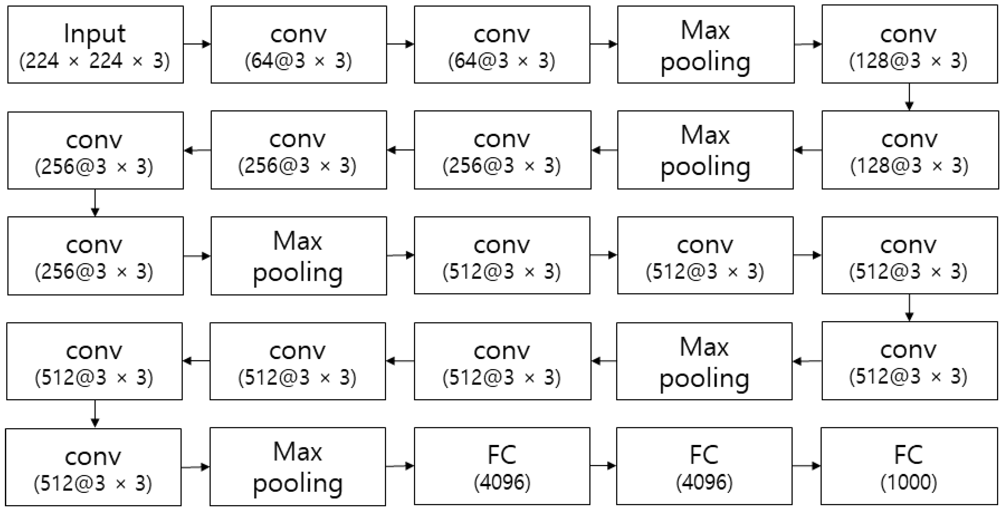
VGGNet is ranked second in the ILSVRC 2014, following GoogLeNet, but it is more widely used than GoogLeNet because it has a significantly simpler structure. VGGNet uses a relatively small 3 × 3 convolution (conv) filter and a 1 × 1 convolution filter, in contrast to AlexNet’s 11 × 11 filters in the first layer and ZFNet’s 7 × 7 filters. When the nonlinear rectified linear unit (ReLU) activation function is applied after the 1 × 1 convolution, the model becomes more discriminative. Additionally, a smaller filter requires less parameters to be learned and results in higher processing speed. In VGGNet, a maxpool with a 2 × 2 kernel size and 2 strides, 2 fully connected (FC) layers with 4096 nodes, 1 FC layer with 1000 nodes, and 1 Softmax layer is used. Two 3 × 3 convolution layers and three 3 × 3 convolution layers have effective receptive fields of 5 × 5 and 7 × 7, respectively. By doubling the number of filters after each maxpool layer, the spatial dimensions are reduced, but the network depth is increased. Originally, VGGNet was designed to investigate how errors are affected by the network depth. There are models with layer depths of 8, 11, 13, 16, and 19 in VGGNet. As the network depth increases, the error decreases, but the error increases if the layer depth exceeds 19. VGGNet uses data augmentation of scale jittering for training and is trained with batch gradient descent using four Nvidia Titan Black graphics processing units for approximately three weeks [19]. Figure 1 shows the structure of VGGNet. In an expression with the form L@M × N, L, M, and N represent the sizes of the map, the row of the kernel, and the column of the kernel, respectively. The @ is a symbol used to separate the map size and filter size here.

2.2. ResNet

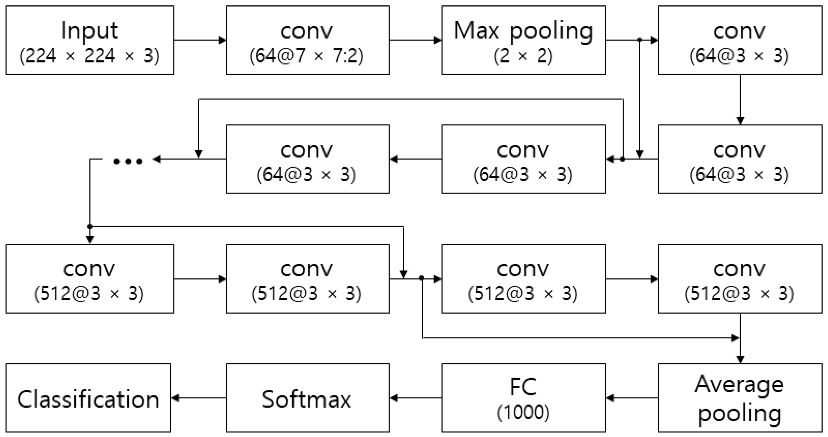
Deep layers of neural networks result in a vanishing gradient, an exploding gradient, and degradation. The vanishing gradient refers to when a propagated gradient becomes too small, and exploding gradient refers to when a propagated gradient becomes too large to train. Degradation indicates that the deep neural network has worse performance than the shallow neural network even though there is no overfitting. ResNet attempts to solve these problems by reusing the input features of the previous layer. Figure 2 shows the structure of ResNet. The output of Y is calculated using the input of X, and the input of X is reused by being added to the output of Y. This is called a skip connection. Then, learning is performed so that ReLU (W × X) converges to 0, indicating that the output of Y is almost equal to X. This reduces the vanishing gradient, and even small changes in the input are delivered to the output. The number of intermediate layers in the section of the skip connection can be set arbitrarily, and ResNet uses this method to stack layers deeply. ResNet is structured according to VGGNet [19] and uses the convolution of 3 × 3 filters, but not pooling or dropout. The pooling is replaced with the convolution of 2 strides. After every two convolutions, the input layer is added at the output [20].

2.3. DenseNet

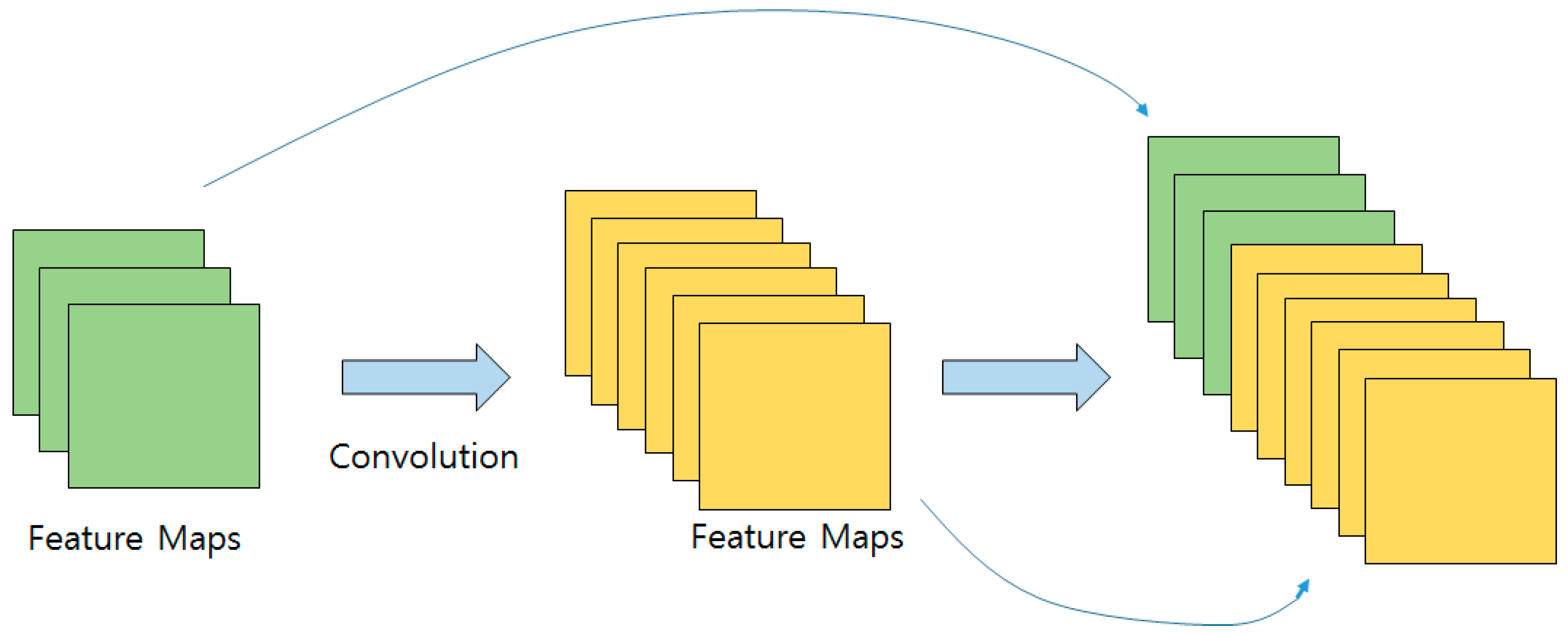
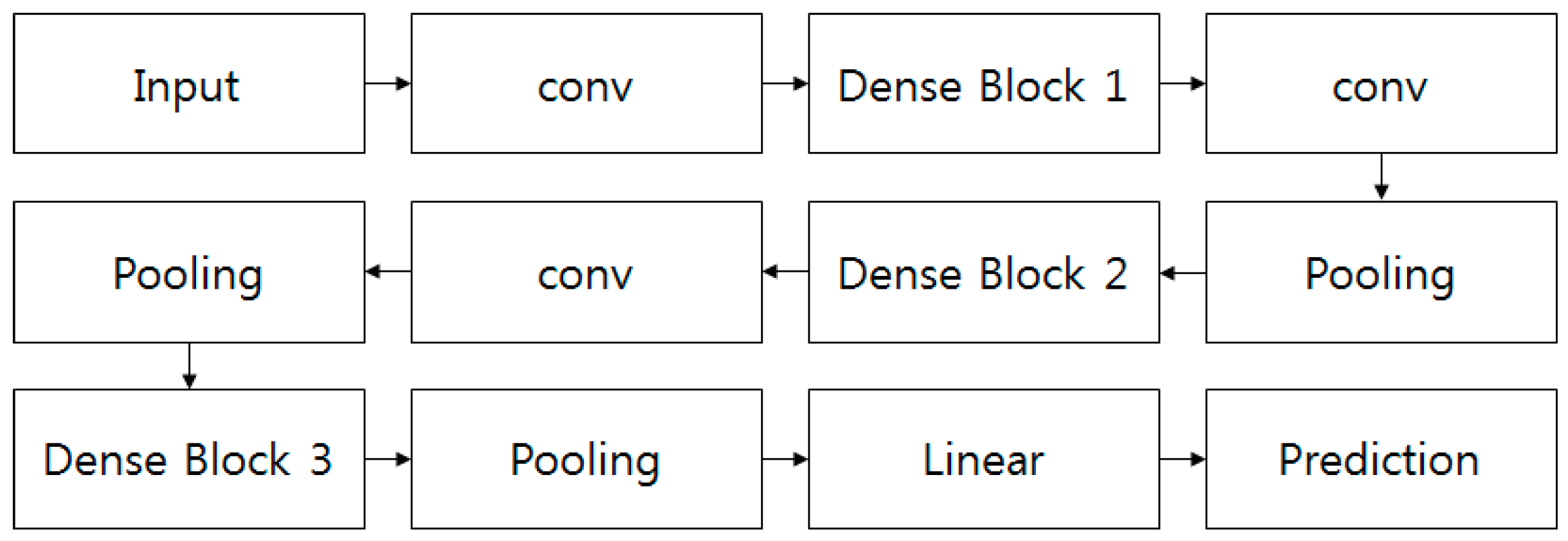
A typical network structure is a sequential combination of convolution, activation, and pooling. In contrast to the typical network, DenseNet solves the degradation problem by introducing a new concept called dense connectivity. DenseNet has approximately 12 filters per layer and uses the dense connectivity pattern to continuously pile up feature maps in previous layers, effectively conveying the information in the early layers to the latter layers. This allows entire feature maps to enter within the network evenly into the last classifier, while simultaneously reducing the total number of parameters, making the network sufficiently learnable. The dense connection also functions as regularization, which reduces the overfitting even for small datasets. Dense connectivity is expressed by Equation (1) and shown in Figure 3. DenseNet divides the entire network into several dense blocks and groups layers with the same size of the feature map into the same dense block. The part of pooling and convolution is called the transition layer. This layer comprises a batch normalization (BN) layer, a 1 × 1 convolution layer for adjusting the dimensions of the feature map, and a 2 × 2 average pooling layer. A bottleneck structure (i.e., BN-ReLU-conv(1)-BN-ReLU-conv(3)), is employed to reduce the computational complexity. Usually, global average pooling is used instead of FC, which most networks have in the last layer. The network is trained via stochastic gradient descent [21]. Figure 4 shows the structure of DenseNet.
x m = H m ( [ x 0 , x 1 , , x m ] )

2.4. InceptionResNetV2

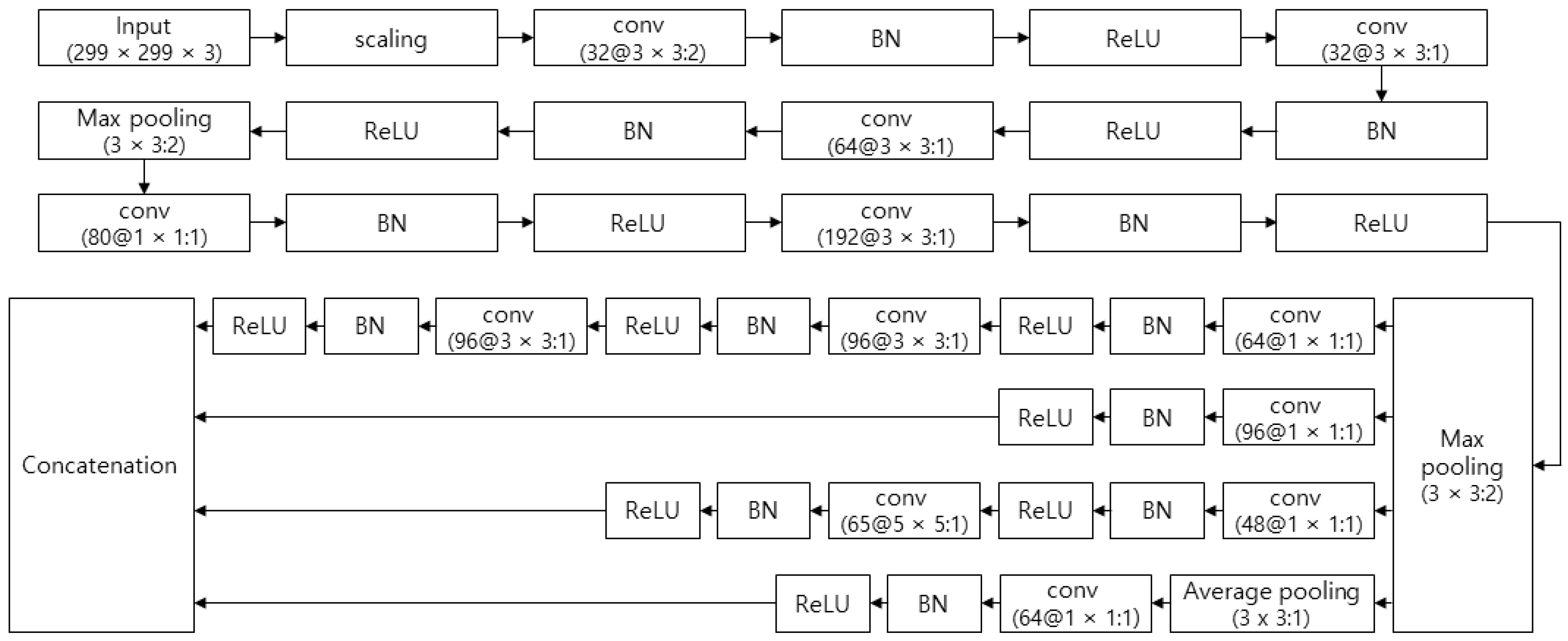
The objective of the inception module is to cover a wide area of the image while maintaining the resolution for smaller information. Thus, convolutions of different sizes from 1 × 1 to 5 × 5 are performed in parallel. The inception module first performs convolution with a 1 × 1 filter and then performs convolutions with filters of different sizes, because the convolution with a 1 × 1 filter reduces the number of feature maps and thus the computational cost. The results of convolutions performed in parallel are concatenated at the output layer of the inception module. The InceptionResNetV2 consists of a stem layer, three types of inception modules (A, B, and C), and two types of reduction modules (A and B). The stem layer is the frontal layer, and the reduction module is used to reduce the size of the feature map in InceptionResNetV2. The inception modules of InceptionResNetV2 are based on the integration of the inception module and the skip connection of ResNet [22]. The stem layer, three types of inception modules (A, B, and C), two types of reduction modules (A and B), and the structure of InceptionResNetV2 are shown in Figure 5, Figure 6, Figure 7 and Figure 8, respectively. In an expression with the form L@M×N:O, L, M, N, and O represent the sizes of the map, the row of the kernel, the column of the kernel, and the stride, respectively.

2.5. Xception

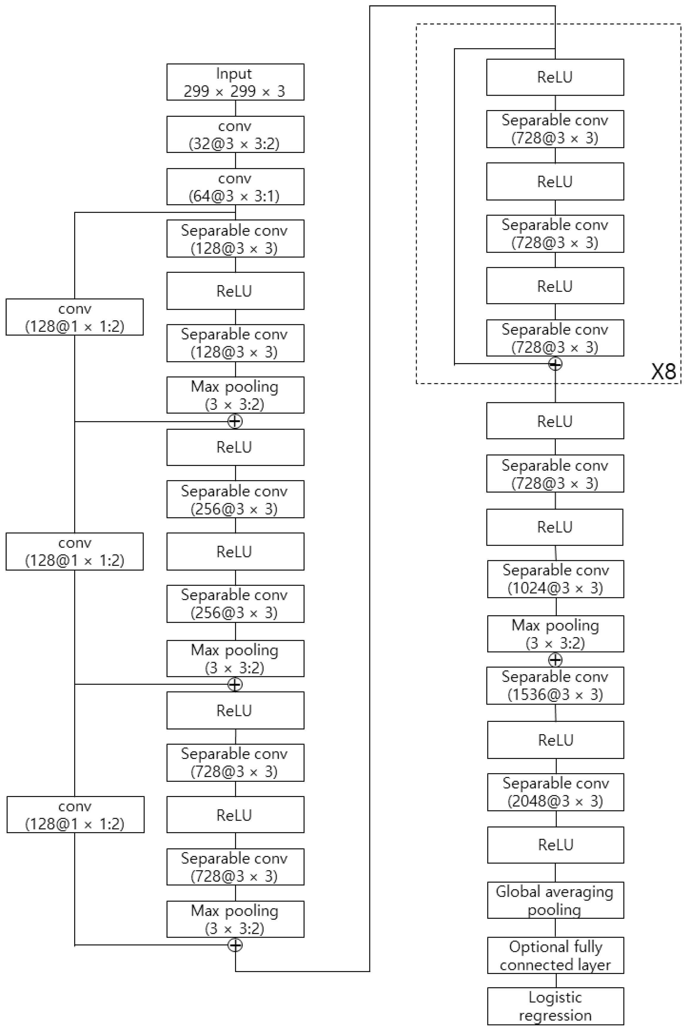
Xception, which is based on inception, seeks to completely separate the search for relationships between channels from the search for regional information on images. In Xception, depth-wise separable convolution is performed for each channel, and the result is projected to the new channel space via 1 × 1 convolution. If the existing convolution created a feature map considering all the channels and local information, the depth-wise convolution creates one feature map for each channel, and then 1 × 1 convolution is performed to adjust the number of feature maps. The 1 × 1 convolution is called the pointwise convolution (point-conv). In inception, each convolution is followed by the nonlinearity of the ReLU; however, in a depth-wise separable convolution, the first convolution is not followed by nonlinearity. Xception has 36 convolution layers in 14 modules for feature extraction. Except for the beginning and end layers, each module has a linear residual connection. In summary, Xception is formed by linearly stacking depth-wise separable convolution layers with residual connections [23]. Figure 6 shows the structure of Xception.

3. Database and Experiment Method

3.1. Construction of Database for Posture Recognition

Training a deep neural network for posture recognition requires a large amount of posture images. Thus, the daily domestic posture database was constructed for posture recognition under the assumption of an environment of domestic service robots. Astra (i.e., an assembly of sensors for color images (red, green, and blue (RGB)), depth images (infrared rays), and sound sources (microphones) made by Orbbec), was used to construct a daily domestic posture database. It senses the depth from 0.6 to 8 m and the color inside a field of view of 60° × 49.5° × 73°. The resolution and frame rate are 640 × 480 pixels and 30 fps, respectively, for the RGB and depth images. The size of Astra is 165 × 30 × 40 m3, its power consumption is 2.4 W (through Universal Serial Bus (USB) 2.0), and it has two microphones. Figure 7 shows the Astra for capturing posture images. It can be developed using the Astra software development kit (SDK) and OpenNI in several operating systems (e.g., Android, Linux, and Windows 7, 8, and 10). The SDK also supports body tracking with a skeleton [38]. To construct the database, a graphical user interface (GUI) for the capture tool was developed using the Microsoft Foundation Class library and the Astra SDK in Windows 7. Figure 8 shows the developed GUI for constructing the posture database.
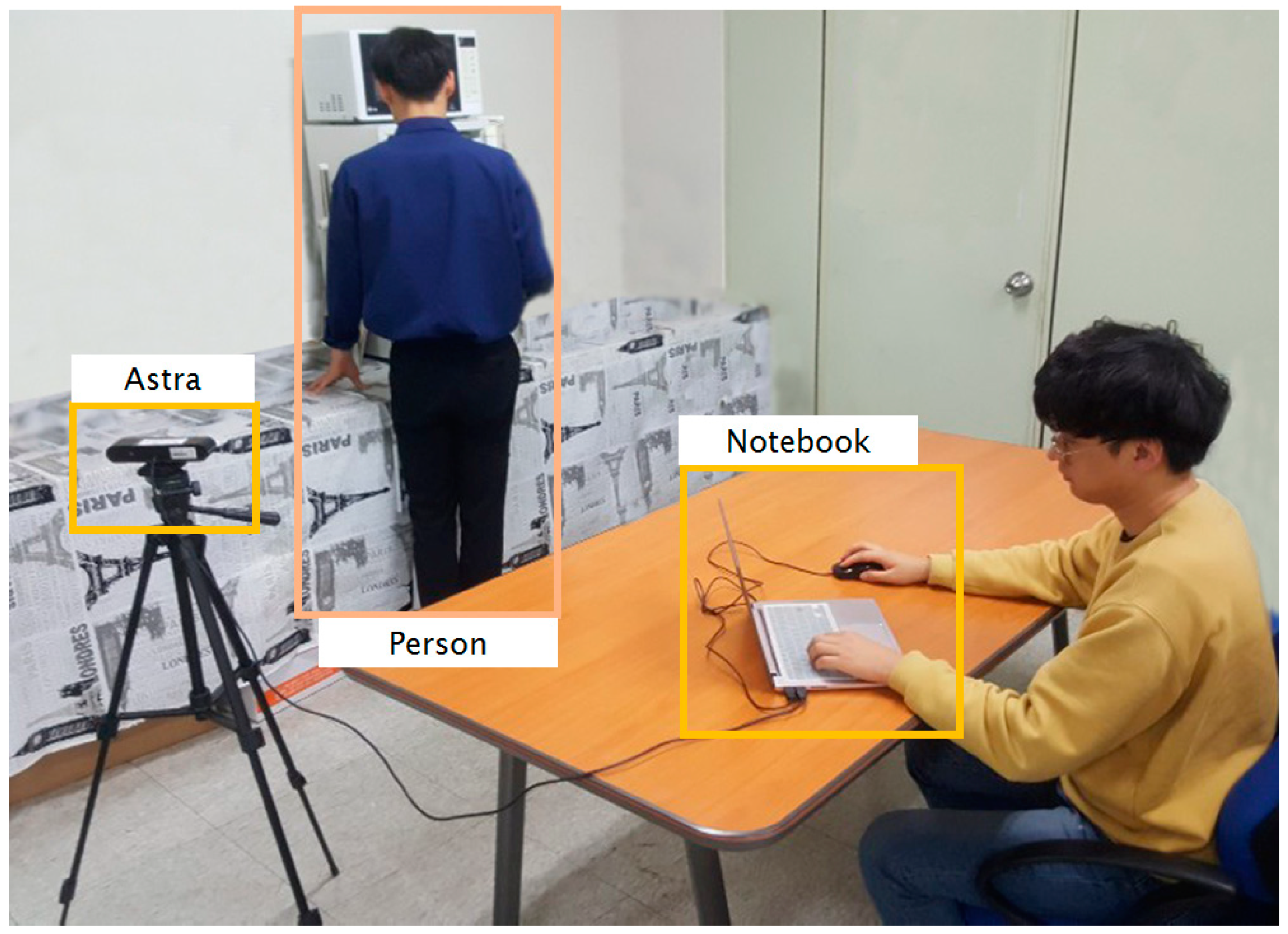
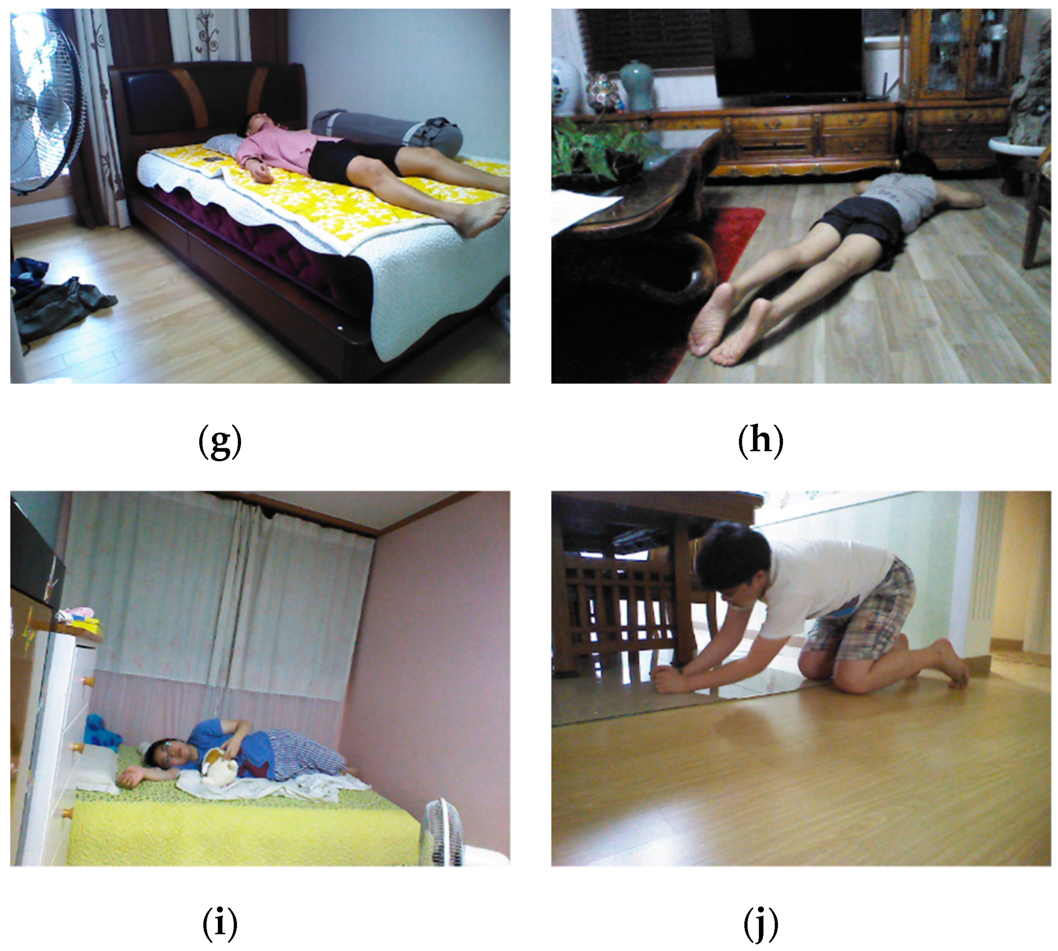
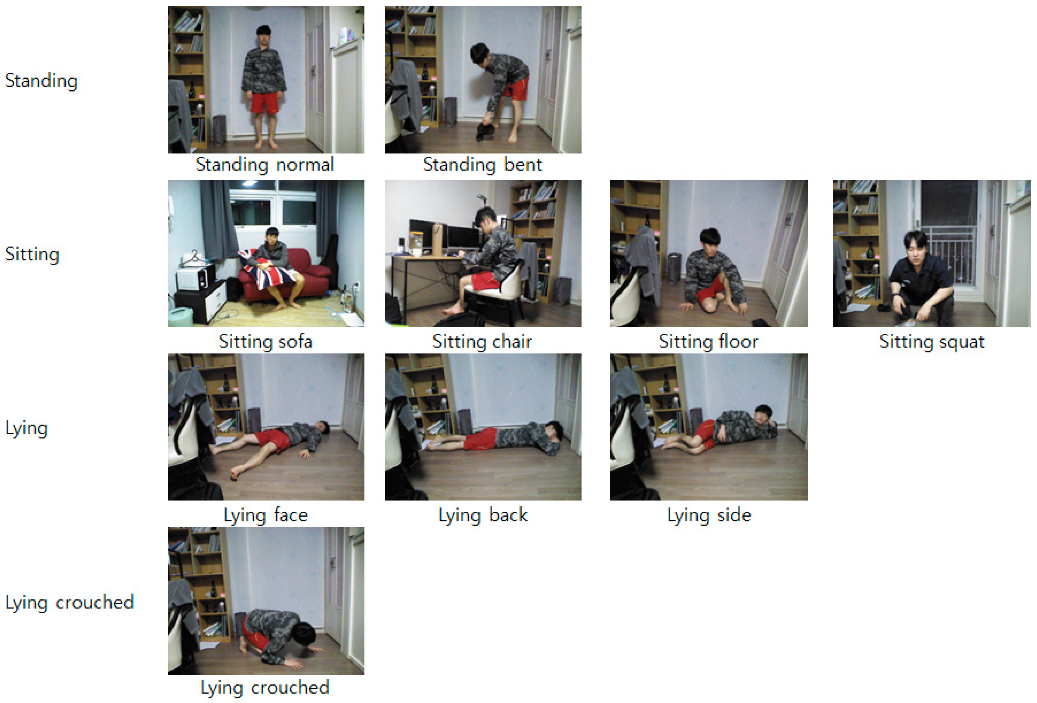
A total of 51 homes participated in the construction of the daily domestic posture database. These homes had a living room, a kitchen, a small room, a dinner table, chairs, a bed, and a sofa. More than two persons in each home equally contributed as subjects for the posture images. Ten postures were defined to construct the daily domestic posture database. The postures were “standing normal”, “standing bent”, “sitting sofa”, “sitting chair”, “sitting floor”, “sitting squat”, “lying face”, “lying back”, “lying side”, and “lying crouched”. Each home generated 100 images per posture, and each image included one subject. Each home generated 1000 posture images (10 postures × 100 images per posture). Thus, the total number of images was 51,000 (1000 posture images × 51 homes). Each image was captured by varying the position, type of room, prop (such as clothes), furniture (such as a chair), pose of the sensor, pose of the person, and small movement. Figure 9 shows the environment for capturing the posture images using Astra. Figure 10 shows examples of posture images captured using Astra.

3.2. Preprocessing Types

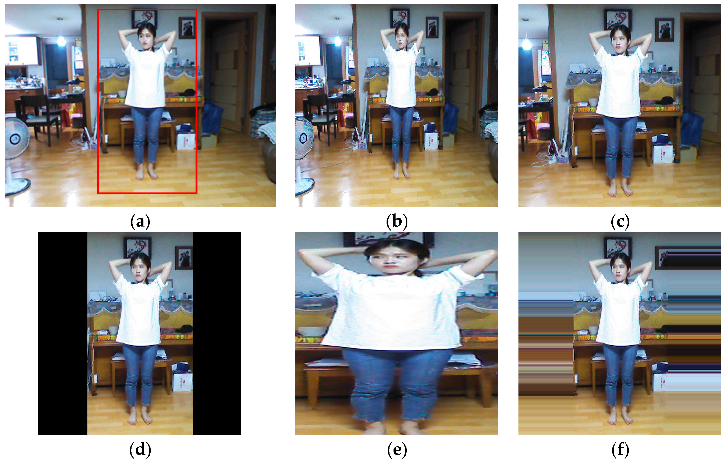
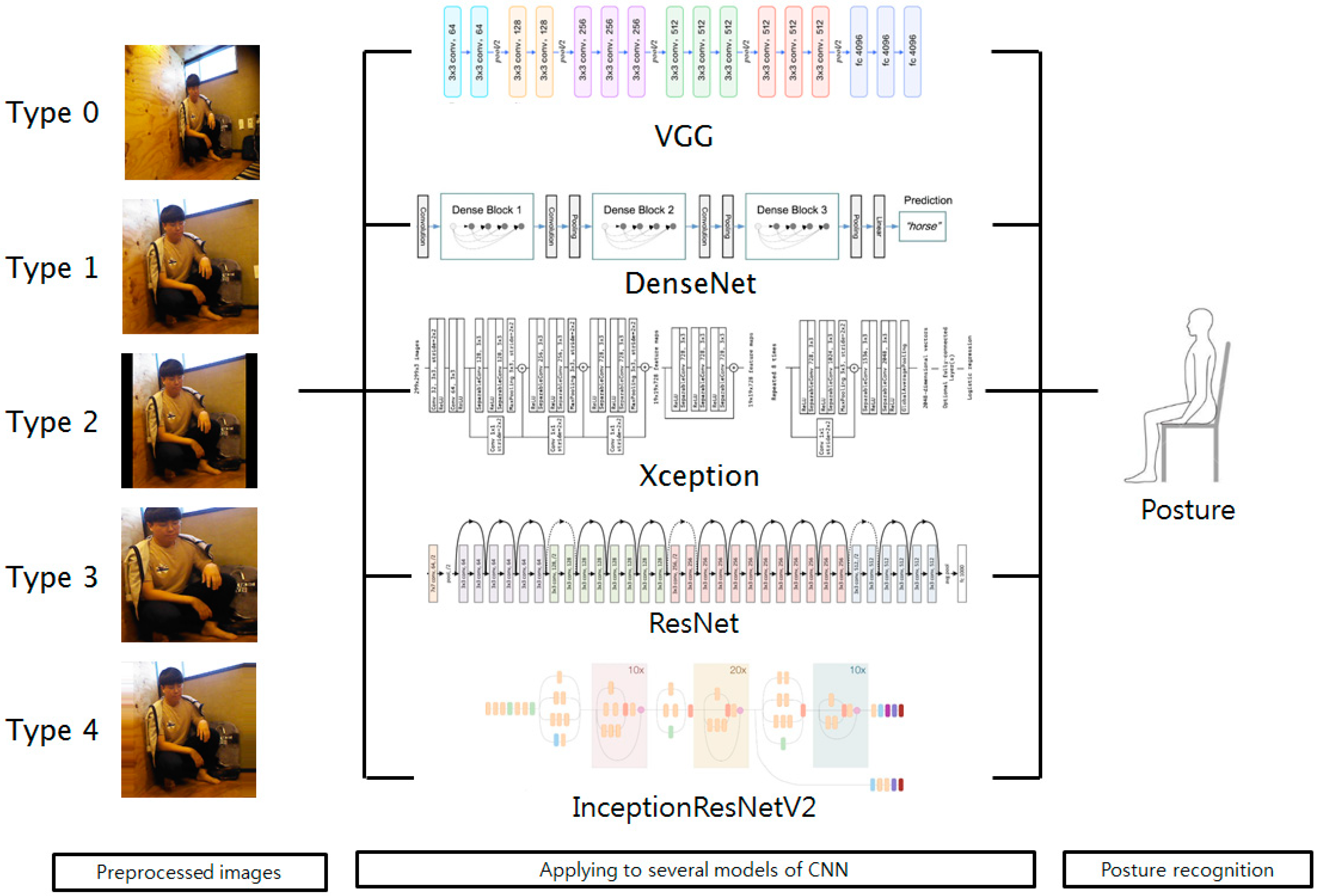
To segment the person images, you only look once (YOLO)-v3 was used as a person detector [39]. After segmenting the person, preprocessing was performed to consider various input methods which have different pros and cons because the neural networks were limited in input as a square fixed image. The pros and cons are based on tightness of person and distortion of person by stretching image. Five types of preprocessing for cropping images were defined to input posture images into the neural network: In type 0, the original image was resized to the size of the input layer. This changed the original ratio of the image. In type 1, the person image was segmented from the original image while satisfying the size of the input layer. The original ratio of the image was maintained. In type 2, the person image was tightly segmented from the original image regardless of the size of the input layer. Then, the person image was resized while maintaining the ratio of the original image until the size of the row or column of the person was equal to the size of the row or column of the input layer, respectively. The extra border due to the difference in the image ratio between the person and the input layer was zero-padded. In type 3, the person image was tightly segmented from the original image regardless of the size of the input layer. Then, the person image was resized to the size of the input layer. This changed the original ratio of the image. In type 4, the person image was tightly segmented from the original image regardless of the size of the input layer. Then, the person image was resized while maintaining the ratio of the original image until the size of the row or column of the person was equal to the size of the row or column of the input layer, respectively. The extra border due to the difference in the image ratio between the person and the input layer was replicated to the edge of the original image. Figure 11 shows the examples of five types of original and preprocessed images.

3.3. Posture Recognition Using Ensemble CNN Models

As more people live alone, there is a need for ways to cope with crime or dying alone. Posture recognition emerged as a solution because it contains some information about the person’s situation. However, posture recognition using the conventional inertial sensor, the sensor is cumbersome to attach to the body. For the elderly, it is difficult to wear the sensor all the time and extra help is needed for them to do so. However, image-based posture recognition through a camera can be applied to the existing camera system and there is no need to attach any sensors. In addition, low-cost webcams can also be applied because the posture is recognized only by the image. It has been difficult to recognize posture by using only two-dimensional images, but recently, deep learning has proved excellent in various fields. We applied the technique to the 2D image based posture recognition. First, a daily domestic posture database was constructed. Then, the posture images were processed to different types of preprocessing. The CNN models were VGG16, VGG19 [19], ResNet50 [20], DenseNet201 [21], InceptionResNetV2 [22], and Xception [23]. Transfer learning is effectively used in cases where a neural network needs to be trained with a small database and there is insufficient time to train the network with new data. In this study, posture recognition was performed by training the CNNs using transfer learning. Most of the parameters used to extract the feature maps were fixed, and only the final FC layers and Softmax were trained. In addition, CNNs were trained by updating all the parameters (nontransfer learning). Figure 12 shows the posture recognition using the preprocessed images for different CNN models. Then CNNs of the deep models and CNNs of the preprocessing types are combined using the majority of outputs and average of scores as ensemble methods. The majority of outputs decides the most voted class among outputs of CNNs. The average of score decides the class with a max score from averaged scores of CNNs. Table 1 and Table 2 show the ensemble methods of majority vote and score average. Figure 13 shows the various ensemble systems by input types and CNN models.
The number of postures is the number of classes. The number of defined postures was 10: “standing normal”, “standing bent”, “sitting sofa”, “sitting chair”, “sitting floor”, “sitting squat”, “lying face”, “lying back”, “lying side”, and “lying crouched”. The 10 posture classes were divided into four categories: standing, sitting, lying, and lying crouched. Instead of 10 and 4 classes, there were 11 and 5 when other images, such as the background, were considered as a separate class. The results of posture recognition under 10, 4, 11, and 5 classes were obtained. The other images were configured by programmatically cropping the original posture images randomly while avoiding the person to the greatest extent possible. These various numbers of classes have the advantage to extract context information. For example, a person does not sleep in a standing posture. Figure 14 shows the four categories.
The posture-recognition performance was evaluated with regard to accuracy, which was defined as the number of correct classifications (CC) divided by the number of total classifications (i.e., the sum of CC and the number of wrong classifications (WC)) [40]:
A c c u r a c y =   C C C C   +   W C  

4. Experimental Results

4.1. Database

The daily domestic posture database was directly constructed from 51 homes using Astra. All homes had a living room, a kitchen, a small room, a dinner table, chairs, a bed, and a sofa. The postures included “standing normal”, “standing bent”, “sitting sofa”, “sitting chair”, “sitting floor”, “sitting squat”, “lying face”, “lying back”, “lying side”, and “lying crouched”. Each home had 100 images per posture, and each image included one subject. Each home had 1000 posture images (10 postures × 100 images per posture). The total number of images was 51,000 (1000 posture images × 51 homes). The images were captured by varying the position, type of room, prop (such as clothes), furniture (such as a chair), pose of the sensor, pose of the person, and small movement. The posture database was constructed with men and women ranging from 19 to 68 years of age. Figure 15 shows the data configuration for the training, validation, and testing. The posture images were subjected to different types of preprocessing. To segment the person image, YOLO-v3 was used as a person detector [39], and the segmented person images were filtered manually. The number of preprocessed posture images for the training was 3910 for standing normal, 3802 for standing bent, 3899 for sitting sofa, 3899 for sitting chair, 3896 for sitting floor, 3859 for sitting squat, 3752 for lying face, 3777 for lying back, 3773 for lying side, 3505 for lying crouched, and 6802 for other images. The number of preprocessed posture images for the validation was 689 for standing normal, 670 for standing bent, 688 for sitting sofa, 687 for sitting chair, 687 for sitting floor, 681 for sitting squat, 662 for lying face, 666 for lying back, 665 for lying side, 618 for lying crouched, and 1200 for other images. The number of preprocessed posture images for the testing was 500 for standing normal, 497 for standing bent, 500 for sitting sofa, 500 for sitting chair, 497 for sitting floor, 498 for sitting squat, 489 for lying face, 489 for lying back, 482 for lying side, 481 for lying crouched, and 2001 for other images. The total number of images for the training, validation, and testing was 44,874, 7913, and 6934, respectively.

4.2. Experimental Results

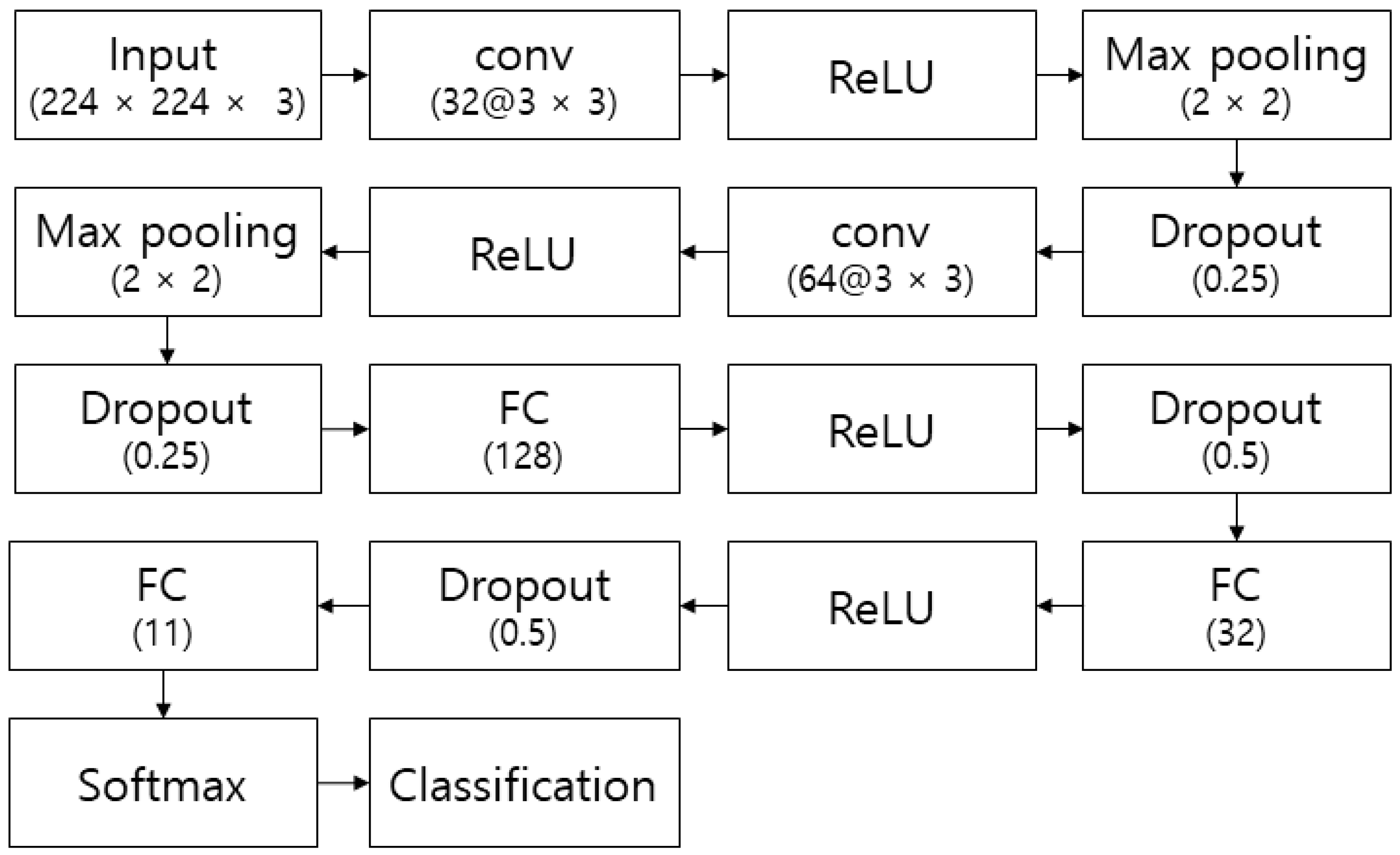
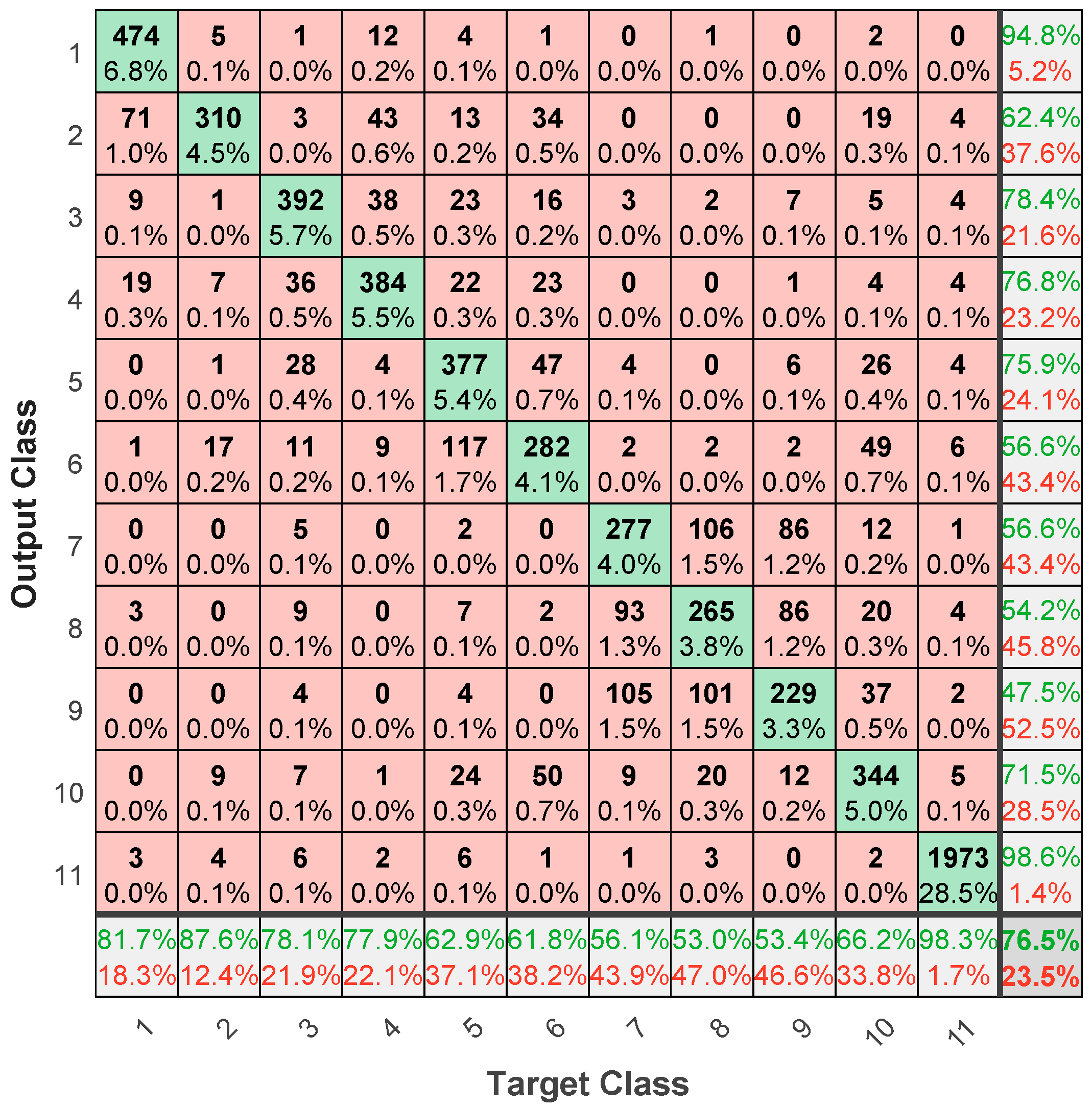
The computer used in the experiment had the following specifications: Intel i7-6850K central processing unit at 3.60 GHz, Nvidia GeForce GTX 1080 Ti, 64 GB of random-access memory, and Windows 10 64-bit operating system. The CNN models used for posture recognition in this study were VGG16, VGG19 [19], ResNet50 [20], DenseNet201 [21], InceptionResNetV2 [22], and Xception [23], which are pre-trained CNNs. A pre-trained CNN can be used for transfer learning when new data need to be classified efficiently. Most of the parameters used to extract the feature maps were fixed, and only the final FC layers and Softmax were trained. A simple CNN (the conventional method) was added to the experiment for performance comparison. The structure of the simple CNN is depicted in Figure 16. The simple CNN was trained by updating all the parameters, because it was not a pre-trained model. Here, the number of postures was the number of classes. The number of defined postures was 10: “standing normal”, “standing bent”, “sitting sofa”, “sitting chair”, “sitting floor”, “sitting squat”, “lying face”, “lying back”, “lying side”, and “lying crouched”. If a class of “other images” (e.g., background) was added to the 10 posture classes, then the number of total classes was 11. The training, validation, and testing data sets for the 11 classes consisted of 44,874, 7913, and 6934 images, respectively. Additionally, the 10 posture classes were divided into four categories: standing, sitting, lying, and lying crouched. If a class for “other images” was added to these four posture classes, the number of total classes was five. The performance for the other numbers of classes was measured through simple mapping of the trained model with the data of 11 classes. The simple CNN was trained with a batch size of 128, 50 epochs, and the RMSProp optimizer [41]. The other pre-trained models were trained via transfer learning with a batch size of 128, 30 epochs, and the Adadelta optimizer [42]. The highest accuracies without data augmentation under transfer learning were 78.35% for VGG19 and type 2 preprocessing with the posture data of 11 classes, 69.89% for VGG19 and type 2 preprocessing with the posture data of 10 classes, 88.86% for VGG19 and type 2 preprocessing with the posture data of five classes, and 88.50% for ResNet50 and type 1 preprocessing with the posture data of four classes. Table 3 presents the classification performance of the CNNs without data augmentation under transfer learning. Figure 17 shows the confusion matrix for VGG19 with type 2 preprocessing, which exhibited the best performance for the posture data of 11 classes without data augmentation under transfer learning. Table 4, Table 5 and Table 6 present the accuracies of the CNNs for the posture data of 10, 5, and 4 classes, respectively, without data augmentation under transfer learning.
Next, the experiment was performed in the same way, but data augmentation was added for the training. The data were augmented with a rotation range of 10, a shear range of 10, a zoom range of 0.2, and a horizontal flip of “true”. The highest accuracies with data augmentation under transfer learning were 76.54% for VGG19 and type 2 preprocessing with the posture data of 11 classes, 67.47% for VGG19 and type 2 preprocessing with the posture data of 10 classes, 87.92% for VGG19 and type 2 preprocessing with the posture data of five classes, and 85.44% for DenseNet201 and type 2 preprocessing with the posture data of four classes. Table 7 presents the classification performance of the CNNs with data augmentation under transfer learning. Figure 18 shows the confusion matrix for VGG19 and type 2 preprocessing, which exhibited the best performance for the posture data of 11 classes with data augmentation under transfer learning. Table 8, Table 9 and Table 10 present the accuracies of the CNNs for the posture data of 10, 5, and 4 classes, respectively, with data augmentation under transfer learning.
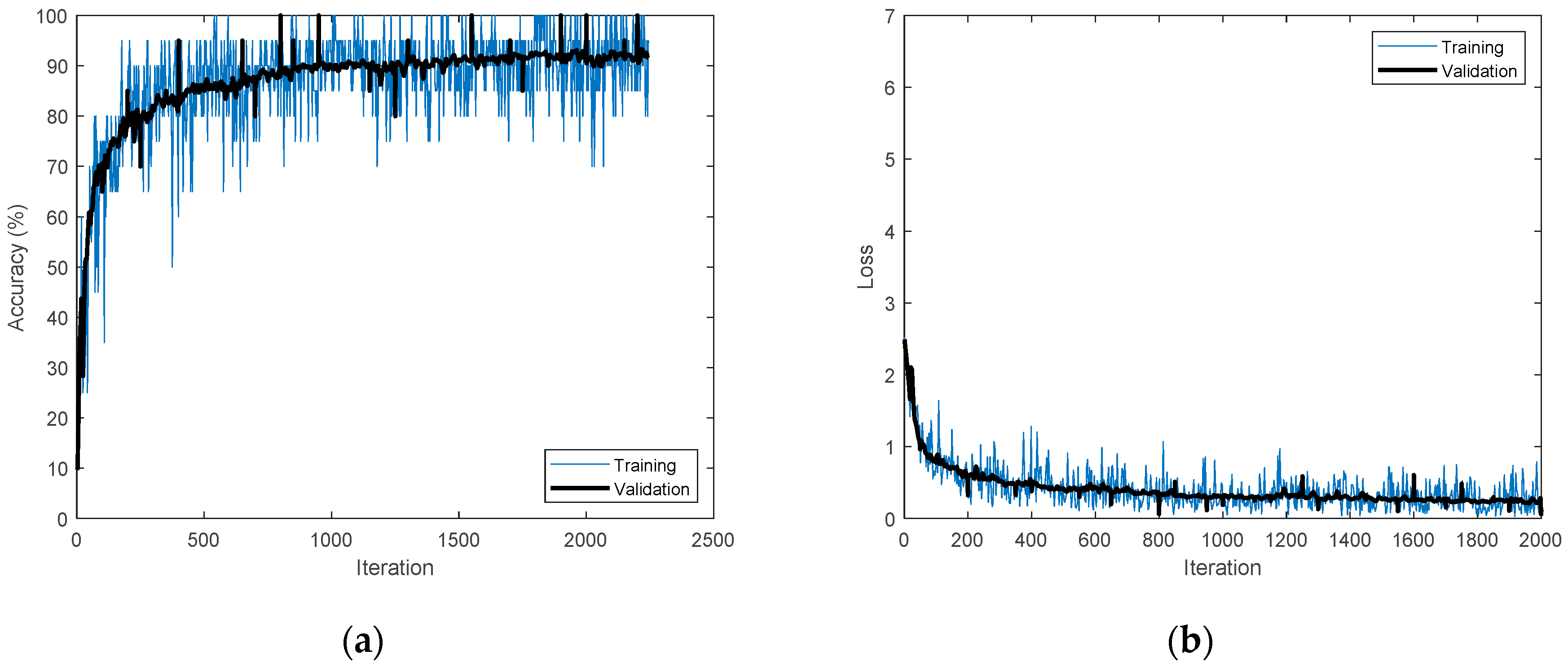
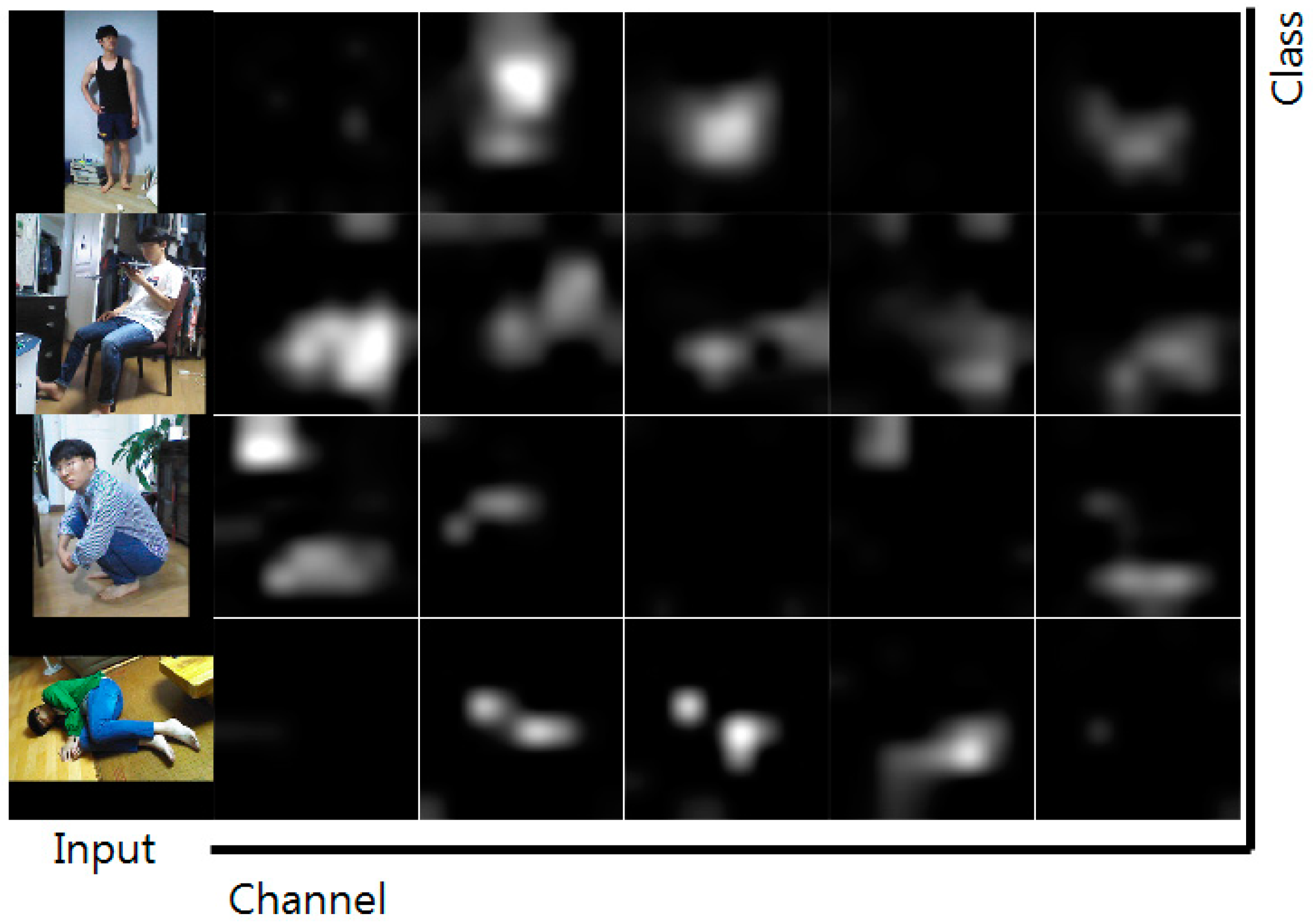
The CNNs were trained via nontransfer learning. VGG19, ResNet50, ResNet101, and InceptionResNetV2 were considered for nontransfer learning. The first three models were trained with a batch size of 60, three epochs, and the Adam optimizer [43]; the last model was trained with a batch size of 20, one epoch, and the Adam optimizer. The highest accuracies were 93.32% for InceptionResNetV2 and type 2 preprocessing with the posture data of 11 classes without data augmentation under nontransfer learning. Table 11 presents the classification performance for 11 classes without augmentation under nontransfer learning. Table 12 presents the training time of a single model for 11 classes without augmentation under nontransfer learning. Figure 19 shows the training process for InceptionResNetV2 and type 2 preprocessing, which exhibited the best performance for the posture data of 11 classes without data augmentation under nontransfer learning. Figure 20 shows the activations for InceptionResNetV2 and type 2 preprocessing. Figure 21 shows the activations of the last ReLU for ResNet50 and type 2 preprocessing.
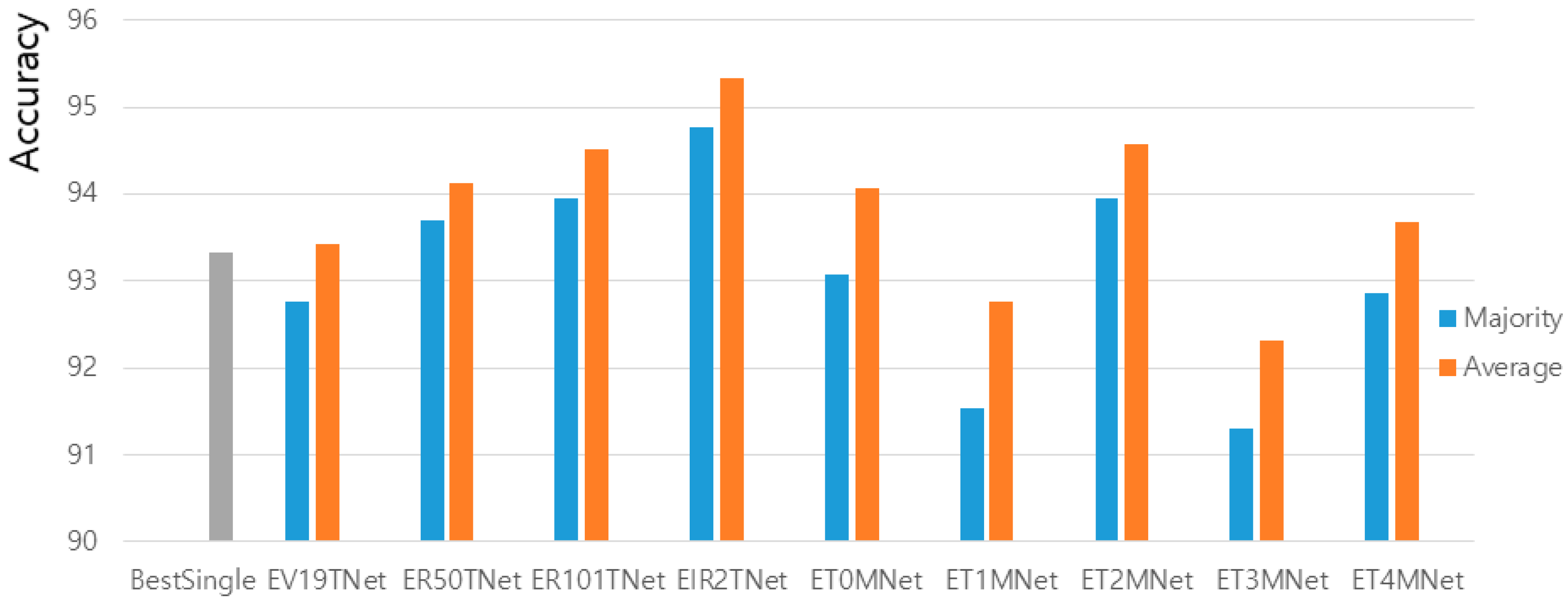
The trained CNN models from Table 11 are combined using the majority of outputs and average of scores. First, the five CNNs trained with different input types are combined under VGG19, ResNet50, ResNet101, and InceptionResNetV2 as EV19TNet, ER50TNet, ER101TNet, and EIR2TNet, respectively. Table 13 describes the classification performance of ensemble deep models designed by input types. Secondly, the four CNNs trained with different models are combined under input types from 0 to 4 as ET0MNet, ET1MNet, ET2MNet, ET3MNet, and ET4MNet, respectively. Table 14 indicates the classification performance of ensemble deep models designed by the pre-trained CNNs. Table 15 indicates the training time of the ensemble system for 11 classes without augmentation under nontransfer learning. In ensemble systems, the highest accuracy is 95.34% of InceptionResNetV2s using average of scores.
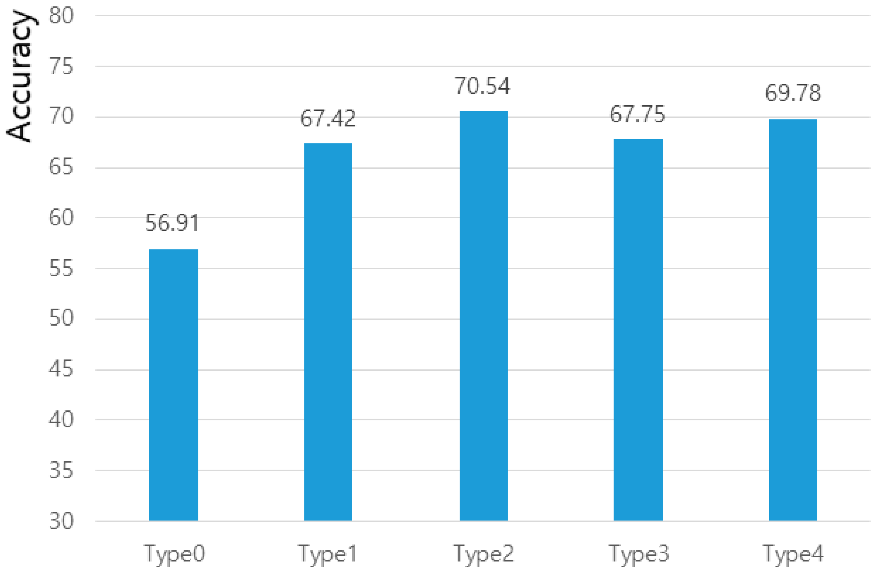
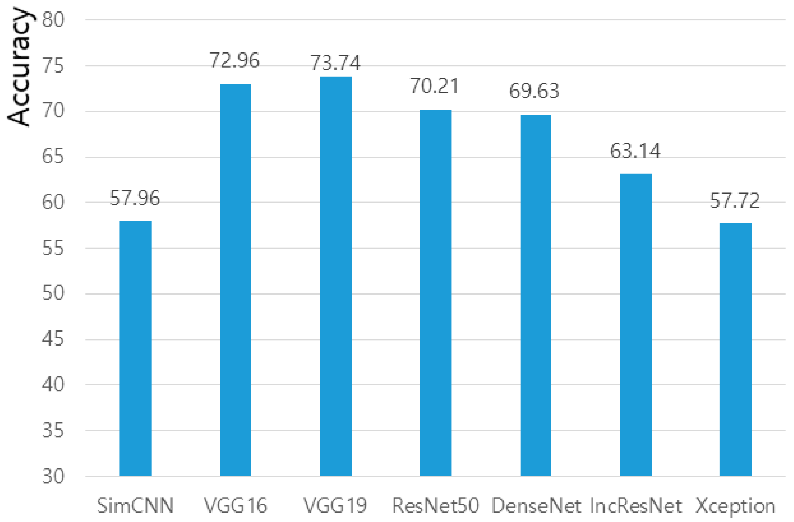
The classification performances listed in Table 3, Table 4, Table 5, Table 6, Table 7, Table 8, Table 9 and Table 10 were computed by average value. Figure 22 shows the average values of classification performance under transfer learning for the different types of preprocessing. The experimental results on preprocessing of type 2 showed 13.63%, 3.12%, 2.79%, and 0.76% higher classification rate than types 0, 1, 3, and 4, respectively. Figure 23 shows a comparison of the average total accuracies for the different models under transfer learning. The ‘SimCNN’, ‘DenseNet’, and ‘IncResNet’ are simple CNN, DenseNet201, and InceptionResNetV2, respectively. The experimental results by VGG19 showed 15.78%, 0.78%, 3.53%, 4.11%, 10.61%, and 16.02% higher classification performance than the simple CNN, VGG16 [19], ResNet50 [20], DenseNet201 [21], InceptionResNetV2 [22], and Xception [23], respectively.
Figure 24 visualizes the classification performance of ensemble deep models from the results listed in Table 13 and Table 14. Here, ‘BestSingle’ is the best result of single models listed in Table 11. As shown in Figure 24, the ensemble deep model by InceptionResNetV2s with average method showed the best classification performance in comparison to other models.

5. Conclusions

We present ensemble deep models designed by pre-trained CNNs and various types of preprocessing for posture recognition under various home environments. The pertained CNNs used in this paper were performed by VGGNet, ResNet, DenseNet, InceptionResNet, and Xception, frequently used in conjunction with deep learning. Finally, we performed systematic experiments from a large posture database constructed by the Electronics and Telecommunications Research Institute (ETRI). The experimental results reveal that the ensemble deep model shows good performance in comparison with the pre-trained CNN itself. Thus, we expect that the presented method will be an important technique to help elderly people from sudden danger in home environments. In future research, we shall perform the research on the behavior recognition of elderly people from a large 3D database for behavior recognition constructed under home service robot environments.

Author Contributions

Conceptualization, Y.-H.B., J.-Y.L., and K.-C.K.; methodology, Y.-H.B., J.-Y.L., and K.-C.K.; software, Y.-H.B., J.-Y.L., D.-H.K., and K.-C.K.; validation, Y.-H.B., J.-Y.L., D.-H.K., and K.-C.K.; formal analysis, Y.-H.B. and K.-C.K.; investigation, Y.-H.B., J.-Y.L., and K.-C.K.; resources, J.-Y.L., D.-H.K., and K.-C.K.; data curation, Y.-H.B., J.-Y.L., D.-H.K., and K.-C.K.; writing—original draft preparation, Y.-H.B.; writing—review and editing, J.-Y.L. and K.-C.K.; visualization, Y.-H.B., J.-Y.L., and K.-C.K.; supervision, K.-C.K.; project administration, J.-Y.L.; funding acquisition, J.-Y.L. All authors have read and agreed to the published version of the manuscript.

Funding

This research was supported by the Basic Science Research Program through the National Research Foundation of Korea (NRF) funded by the Ministry of Education (No. 2017R1A6A1A03015496). This work was supported by the ICT R&D program of MSIT/IITP (2017-0-00162, Development of Human-care Robot Technology for Aging Society).

Conflicts of Interest

The authors declare no conflict of interest.

References

  1. Park, J.H.; Song, K.H.; Kim, Y.S. A kidnapping detection using human pose estimation in intelligent video surveillance systems. J. Korea Soc. Comput. Inf. 2018, 23, 9–16. [Google Scholar]
  2. Qiang, B.; Zhang, S.; Zhan, Y.; Xie, W.; Zhao, T. Improved convolutional pose machines for human pose estimation using image sensor data. Sensors 2019, 19, 718. [Google Scholar] [CrossRef] [PubMed] [Green Version]
  3. Huang, Z.; Liu, Y.; Fang, Y.; Horn, B.K.P. Video-Based Fall Detection for Seniors with Human Pose Estimation. In Proceedings of the 4th International Conference on Universal Village, Boston, MA, USA, 21–24 October 2018; pp. 1–4. [Google Scholar]
  4. Chan, K.C.; Koh, C.K.; Lee, C.S.G. An automatic design of factors in a human-pose estimation system using neural networks. IEEE Trans. Syst. Man Cybern. Syst. 2016, 46, 875–887. [Google Scholar] [CrossRef]
  5. Veges, M.; Varga, V.; Lorincz, A. 3D human pose estimation with siamese equivariant embedding. Neurocomputing 2019, 339, 194–201. [Google Scholar] [CrossRef]
  6. Stommel, M.; Beetz, M.; Wu, W. Model-free detection, encoding, retrieval, and visualization of human poses from Kinect data. IEEE Asme Trans. Mechatron. 2015, 20, 865–875. [Google Scholar] [CrossRef]
  7. Shum, H.P.H.; Ho, E.S.L.; Jiang, Y.; Takagi, S. Real-time posture reconstruction for Microsoft Kinect. IEEE Trans. Cybern. 2013, 43, 1357–1369. [Google Scholar] [CrossRef]
  8. Lee, J.; Joo, H.; Lee, J.; Chee, Y. Automatic classi?cation of squat posture using inertial sensors: Deep learning approach. Sensors 2020, 20, 361. [Google Scholar] [CrossRef] [Green Version]
  9. Chowdhury, I.R.; Saha, J.; Chowdhury, C. Detailed Activity Recognition with Smartphones. In Proceedings of the Fifth International Conference on Emerging Applications of Information Technology, Kolkata, India, 12–13 January 2018; pp. 1–4. [Google Scholar]
  10. Wu, Z.; Zhang, J.; Chen, K.; Fu, C. Yoga posture recognition and quantitative evaluation with wearable sensors based on two-stage classifer and prior bayesian network. Sensors 2019, 19, 5129. [Google Scholar] [CrossRef] [Green Version]
  11. Idris, M.I.; Zabidi, A.; Yassun, I.M.; Ali, M.S.A.M. Human Posture Recognition Using Android Smartphone and Artificial Neural Network. In Proceedings of the IEEE Control and System Gradate Research Colloquium, Shah Alam, Malaysia, 10–11 August 2015; pp. 120–124. [Google Scholar]
  12. Pak, M.S.; Kim, S.H. A Review of Deep Learning in Image Recognition. In Proceedings of the International Conference on Computer Applications and Information Processing Technology, Kuta Bali, Indonesia, 8–10 August 2017; pp. 1–3. [Google Scholar]
  13. Diao, W.; Sun, X.; Zheng, X.; Dou, F.; Wang, H.; Fu, K. Efficient saliency-based object detection in remote sensing images using deep belief networks. IEEE Geosci. Remote Sens. Lett. 2016, 13, 137–141. [Google Scholar] [CrossRef]
  14. Sasaki, H.; Horiuchi, T.; Kato, S. A Study on Vision-Based Mobile Robot Learning by Deep Q-Network. In Proceedings of the Annual Conference of Society of Instrument Control Engineers, Kanazawa, Japan, 19–22 September 2017; pp. 799–804. [Google Scholar]
  15. Chang, C.H. Deep and shallow architecture of multilayer neural networks. IEEE Neural Netw. Learn. Syst. 2015, 26, 2477–2486. [Google Scholar] [CrossRef]
  16. Mou, L.; Ghamisi, P.; Zhu, X.X. Deep recurrent neural networks for hyperspectral image classification. IEEE Geosci. Remote Sens. 2017, 55, 3639–3655. [Google Scholar] [CrossRef] [Green Version]
  17. Callet, P.L.; Viard-Gaudin, C.; Barba, D. A convolutional neural network approach for objective video quality assessment. IEEE Neural Netw. 2006, 17, 1316–1327. [Google Scholar] [CrossRef] [PubMed]
  18. Hou, J.C.; Wang, S.S.; Lai, Y.H.; Tsao, Y.; Chang, H.W.; Wang, H.M. Audio-visual speech enhancement using multimodal deep convolutional neural networks. IEEE Emerg. Top. Comput. Intell. 2018, 2, 117–128. [Google Scholar] [CrossRef] [Green Version]
  19. Simonyan, K.; Zisserman, A. Very deep convolutional networks for large-scale image recognition. arXiv 2015, arXiv:1409.1556v6. Available online: https://arxiv.org/abs/1409.1556 (accessed on 5 December 2019).
  20. He, K.; Zhang, X.; Ren, S.; Sun, J. Deep Residual Learning for Image Recognition. In Proceedings of the IEEE Conference on Computer Vision and Pattern Recognition, Las Vegas, NV, USA, 27–30 June 2016; pp. 770–778. [Google Scholar]
  21. Huang, G.; Liu, Z.; Maaten, L.V.D.; Weinberger, K.Q. Densely connected convolutional networks. arXiv 2018, arXiv:1608.06993v5. Available online: https://arxiv.org/abs/1608.06993 (accessed on 5 December 2019).
  22. Szegedy, C.; Ioffe, S.; Vanhoucke, V. Inception-v4, Inception-ResNet and the impact of residual connections on learning. arXiv 2016, arXiv:1602.07261v2. Available online: https://arxiv.org/abs/1602.07261 (accessed on 5 December 2019).
  23. Chollet, F. Xception: Deep learning with depthwise separable convolutions. arXiv 2017, arXiv:1610.02357v3. Available online: https://arxiv.org/abs/1610.02357 (accessed on 8 December 2019).
  24. Shao, L.; Zhu, F.; Li, X. Transfer learning for visual categorization: A survey. IEEE Neural Netw. Learn. Syst. 2015, 26, 1019–1034. [Google Scholar] [CrossRef]
  25. Tompson, J.; Jain, A.; LeCun, Y.; Bregler, C. Joint training of a convolutional network and a graphical model for human pose estimation. arXiv 2014, arXiv:1406.2984v2. Available online: https://arxiv.org/abs/1406.2984 (accessed on 8 December 2019).
  26. Carreira, J.; Agrawal, P.; Fragkiadaki, K.; Malik, J. Human pose estimation with iterative error feedback. arXiv 2016, arXiv:1507.06550v3. Available online: https://arxiv.org/abs/1507.06550 (accessed on 8 December 2019).
  27. Pishchulin, L.; Insafutdinov, E.; Tang, S.; Andres, B.; Andriluka, M.; Gehler, P.; Schiele, B. DeepCut: Joint subset partition and labeling for multi person pose estimation. arXiv 2016, arXiv:1511.06645v2. Available online: https://arxiv.org/abs/1511.06645 (accessed on 8 December 2019).
  28. Girshick, R. Fast R-CNN. arXiv 2015, arXiv:1504.08083v2. Available online: https://arxiv.org/abs/1504.08083 (accessed on 8 December 2019).
  29. Insafutdinov, E.; Pishchulin, L.; Andres, B.; Andriluka, M.; Schiele, B. DeeperCut: A deeper, stronger, and faster multi-person pose estimation model. Adv. Concepts Intell. Vis. Syst. 2016, 9910, 34–50. [Google Scholar]
  30. Georgakopoulos, S.V.; Kottari, K.; Delibasis, K.; Plagianakos, V.P.; Maglogiannis, I. Pose recognition using convolutional neural networks on omni-directional images. Neurocomputing 2018, 280, 23–31. [Google Scholar] [CrossRef]
  31. Liu, Y.; Xu, Y.; Li, S.B. 2-D Human Pose Estimation from Images Based on Deep Learning: A Review. In Proceedings of the 2nd IEEE Advanced Information Management, Communicates, Electronic and Automation Control Conference, Xi’an, China, 25–27 May 2018; pp. 462–465. [Google Scholar]
  32. Lee, J.N.; Byeon, Y.H.; Kwak, K.C. Design of ensemble stacked auto-encoder for classification of horse gaits with MEMS inertial sensor technology. Micromachines 2018, 9, 411. [Google Scholar] [CrossRef] [PubMed] [Green Version]
  33. Maguolo, G.; Nanni, L.; Ghidoni, S. Ensemble of convolutional neural networks trained with different activation features. arXiv 2019, arXiv:1905.02473v4. Available online: https://arxiv.org/abs/1905.02473 (accessed on 10 December 2019).
  34. Kim, M.G.; Pan, S.B. Deep learning based on 1-D ensemble networks using ECG for real-time user recognition. IEEE Trans. Ind. Inform. 2019, 15, 5656–5663. [Google Scholar] [CrossRef]
  35. Kahlouche, S.; Ouadah, N.; Belhocine, M.; Boukandoura, M. Human Pose Recognition and Tacking Using RGB-D Camera. In Proceedings of the 8th International Conference on Modelling, Identification and Control, Algiers, Algeria, 15–17 November 2016; pp. 520–525. [Google Scholar]
  36. Na, Y.J.; Wang, C.W.; Jung, H.Y.; Ho, J.G.; Choi, Y.K.; Min, S.D. Real-Time Sleep Posture Recognition Algorithm Using Kinect System. In Proceedings of the Korean Institute of Electrical Engineers Conference on Biomedical System, Hoengseong, Korea, 15–17 February 2016; pp. 27–30. [Google Scholar]
  37. Kim, S.C.; Cha, J.H. Posture Recognition and Spatial Cognition with Hybrid Sensor. In Proceedings of the Korean Society of Precision Engineering Conference, Jeju, Korea, 29–31 May 2013; pp. 971–972. [Google Scholar]
  38. Giancola, S.; Valenti, M.; Sala, R. A survey on 3D cameras: Metrological comparison of time-of-flight, structured-light and active stereoscopy technologies. In Springer Briefs in Computer Science; Zdonik, S., Shekhar, S., Wu, X., Jain, L.C., Padua, D., Shen, X.S., Furht, B., Subrahmanian, V.S., Hebert, M., Ikeuchi, K., et al., Eds.; Springer Nature: Cham, Switzerland, 2018; pp. 29–39. ISBN 9783319917603. [Google Scholar]
  39. Redmon, J.; Farhadi, A. YOLOv3: An incremental improvement. arXiv 2018, arXiv:1804.02767v1. Available online: https://arxiv.org/abs/1804.02767 (accessed on 10 December 2019).
  40. Choi, H.S.; Lee, B.H.; Yoon, S.R. Biometric authentication using noisy electrocardiograms acquired by mobile sensors. IEEE Access 2016, 4, 1266–1273. [Google Scholar] [CrossRef]
  41. RMSprop Optimization Algorithm for Gradient Descent with Neural Networks. Available online: https://insidebigdata.com/2017/09/24/rmsprop-optimization-algorithm-gradient-descent-neural-networks/ (accessed on 16 May 2019).
  42. Zeiler, M.D. Adadelta: An adaptive learning rate method. arXiv 2012, arXiv:1212.5701v1. Available online: https://arxiv.org/abs/1212.5701 (accessed on 13 December 2019).
  43. Kingma, D.P.; Ba, J. Adam: A method for stochastic optimization. arXiv 2017, arXiv:1412.6980v9. Available online: https://arxiv.org/abs/1412.6980 (accessed on 13 December 2019).
Figure 1. Structure of VGGNet. FC, fully connected.
Applsci 10 01287 g001
Figure 2. Structure of ResNet.
Applsci 10 01287 g002
Figure 3. Dense connectivity.
Applsci 10 01287 g003
Figure 4. Structure of DenseNet.
Applsci 10 01287 g004
Figure 5. Stem layer of InceptionResNetV2. BN, batch normalization; ReLU, rectified linear unit.
Applsci 10 01287 g005
Figure 6. Structure of Xception.
Applsci 10 01287 g006
Figure 7. Astra camera for capturing posture images. RBG, red, blue, green; USB, Universal Serial Bus.
Applsci 10 01287 g007
Figure 8. Graphical user interface (GUI) for constructing the posture database.
Applsci 10 01287 g008
Figure 9. Environment for capturing posture images using Astra.
Applsci 10 01287 g009
Figure 10. Examples of posture images captured from Astra camera in various home environments: (a) standing normal; (b) standing bent; (c) sitting sofa; (d) sitting chair; (e) sitting floor; (f) sitting squat; (g) lying face; (h) lying back; (i) lying side; (j) lying crouched.
Applsci 10 01287 g010aApplsci 10 01287 g010b
Figure 11. Examples of five types of original and preprocessed images: (a) original image; (b) type 0; (c) type 1; (d) type 2; (e) type 4; (f) type 5.
Applsci 10 01287 g011
Figure 12. Ensemble deep models using the preprocessed images with different convolutional neural network (CNN) models.
Applsci 10 01287 g012
Figure 13. Various ensemble deep models by input types and the pre-trained CNNs.
Applsci 10 01287 g013
Figure 14. Examples of four categories with 10 postures.
Applsci 10 01287 g014
Figure 15. Data configuration for training, validation, and testing data set.
Applsci 10 01287 g015
Figure 16. Structure of the simple CNN.
Applsci 10 01287 g016
Figure 17. Confusion matrix for VGG19 with preprocessing of type 2 without data augmentation.
Applsci 10 01287 g017
Figure 18. Confusion matrix for VGG19 with preprocessing of type 2.
Applsci 10 01287 g018
Figure 19. Training process for InceptionResNetV2 with preprocessing of type 2: (a) accuracy; (b) loss.
Applsci 10 01287 g019
Figure 20. Activations for InceptionResNetV2 with preprocessing of type 2, which exhibited the best performance for the posture data of 11 classes without data augmentation under nontransfer learning: (a) activations of first convolution; (b) activations of last convolution.
Applsci 10 01287 g020
Figure 21. Activations of the last ReLU for InceptionResNetV2 with preprocessing of type 2, which exhibited the best performance for the posture data of 11 classes without data augmentation under nontransfer learning.
Applsci 10 01287 g021
Figure 22. Comparison of the average total accuracies for the different types of preprocessing under transfer learning.
Applsci 10 01287 g022
Figure 23. Comparison of the average total accuracies for the different models under transfer learning.
Applsci 10 01287 g023
Figure 24. Performance comparison by various ensemble deep models.
Applsci 10 01287 g024
Table 1. Ensemble method of majority vote.
1.
Net results scores of each class as 1 × n matrix.
s c = [ x 1   x 2   x 3   x n ]
2.
Get the outputs by picking the class to the max value in scores as one hot matrix.
o c = [ 0   0   1   0 ]
3.
Sum the one hot matrix of all classifiers.
v = c = 1 C o c
4.
Get the final output by picking the class to the max value in sum of one hot matrix.
o v = [ 1   0   0 0 ]
Table 2. Ensemble method of score average.
1.
Net results scores of each class as 1 × n matrix.
s c = [ x 1   x 2   x 3   x n ]
2.
Calculate the average of scores of all classifiers.
a = 1 C c = 1 C s c
3.
Get the final output by picking the class to the max value in average of scores.
o a = [ 1   0   0 0 ]
Table 3. Classification performance of the CNNs without data augmentation under transfer learning (11 classes).
Single Model (%)Type 0Type 1Type 2Type 3Type 4
SimpleCNNTraining91.5070.8281.1285.4268.87
Validation75.6558.7063.7457.9859.34
Testing45.8061.0367.1860.8563.48
VGG16Training89.4088.4491.7285.8785.76
Validation74.5074.6276.9272.6574.59
Testing63.4470.1276.6470.7875.31
VGG19Training90.0991.1789.5683.0686.18
Validation74.5174.2277.1873.1274.93
Testing64.8769.8278.3571.4674.94
ResNet50Training60.0371.5660.6767.4868.05
Validation58.4469.1059.9265.6165.64
Testing55.6066.8357.9265.5561.81
DenseNet201Train62.1770.5262.5370.6559.44
Validation60.6867.5661.2768.4458.34
Test54.5164.1655.8866.5150.68
InceptionResNetV2Train44.9855.6355.1059.6856.01
Validation43.8653.6754.7159.3955.90
Test40.2849.3553.2059.6152.48
XceptionTrain43.5657.1251.1857.2156.52
Validation42.3454.7349.6255.9854.15
Test34.7450.0346.0954.6652.32
Table 4. Classification performance of the CNNs without data augmentation under transfer learning (10 classes).
Single Model (%)Type 0Type 1Type 2Type 3Type 4
SimpleCNN25.3648.1653.8851.6351.54
VGG1648.9562.6367.3463.6566.79
VGG1951.1861.9469.8964.7166.95
ResNet5053.1266.3062.7660.3664.90
DenseNet20155.0162.5961.0361.3757.10
InceptionResNetV243.7956.2455.6054.6858.26
Xception36.1652.2753.6950.0355.27
Table 5. Classification performance of the CNNs without data augmentation under transfer learning (5 classes).
Single Model (%)Type 0Type 1Type 2Type 3Type 4
Raw56.2974.4079.5372.9278.46
VGG1675.5279.8288.0583.3685.84
VGG1976.2380.6788.8683.6786.47
ResNet5074.9184.3578.7382.3980.43
DenseNet20170.8779.7377.0881.7373.60
InceptionResNetV257.9668.7672.9974.7174.08
Xception52.0866.7266.1967.1969.41
Table 6. Classification performance of the CNNs without data augmentation under transfer learning (4 classes).
Single Model (%)Type 0Type 1Type 2Type 3Type 4
Raw46.4069.9474.5170.3174.99
VGG1669.7177.7385.2582.1783.32
VGG1970.7178.6486.3482.6384.51
ResNet5078.2588.5086.9983.4687.08
DenseNet20175.3682.7385.5982.4483.35
InceptionResNetV264.6777.9679.4675.4983.11
Xception57.4172.3876.0067.5875.63
Table 7. Classification performance of the CNNs with data augmentation under transfer learning (11 classes).
Single Model (%)Type 0Type 1Type 2Type 3Type 4
SimpleCNNTraining69.8966.3565.5462.1167.34
Validation62.9259.4763.0243.4261.97
Testing42.7052.6364.3550.0060.15
VGG16Training82.0782.7786.7881.4082.16
Validation73.7373.0276.4072.3774.29
Testing61.6267.3576.0568.8472.01
VGG19Training82.6983.9885.5782.8083.27
Validation73.1373.2176.7472.6474.14
Testing62.8667.3976.5469.7173.67
ResNet50Training58.3367.8957.7666.1062.82
Validation56.7464.8555.8463.0761.36
Testing53.4360.6749.6363.0454.15
DenseNet201Training68.3371.8473.1267.9667.00
Validation66.3517.2770.0318.3463.61
Testing57.0466.4164.2561.0854.24
InceptionResNetV2Training50.2259.0458.6858.9960.40
Validation48.1015.0556.7815.1558.42
Testing44.5852.5552.9156.6957.27
XceptionTraining44.3157.9754.0855.3657.00
Validation42.8515.0909.5114.3055.22
Testing35.1552.5445.6353.5350.94
Table 8. Classification performance of the CNNs with data augmentation under transfer learning (10 classes).
Single Model (%)Type 0Type 1Type 2Type 3Type 4
SimpleCNN24.2038.3549.9540.1746.41
VGG1646.9961.1966.7861.6563.88
VGG1948.9460.4567.4762.4065.12
ResNet5048.8564.0058.6958.2259.42
DenseNet20154.6663.7564.2459.6760.11
InceptionResNetV246.2255.9653.2153.9359.68
Xception38.0254.3650.4347.6753.82
Table 9. Classification performance of the CNNs with data augmentation under transfer learning (5 classes).
Single Model (%)Type 0Type 1Type 2Type 3Type 4
Raw51.4360.4378.7161.9673.37
VGG1672.3778.4487.5282.1983.76
VGG1974.4478.1987.9282.4984.83
ResNet5069.5478.7073.4778.4975.94
DenseNet20171.0080.7081.1779.7975.83
InceptionResNetV261.6771.7173.7472.3477.13
Xception52.5068.6566.3866.5568.93
Table 10. Classification performance of the CNNs with data augmentation under transfer learning (4 classes).
Single Model (%)Type 0Type 1Type 2Type 3Type 4
Raw42.3153.7273.5558.9768.33
VGG1666.1377.5084.7581.1581.78
VGG1968.8376.7185.2481.2282.46
ResNet5070.8585.3785.0579.4684.69
DenseNet20173.1482.7285.4483.6884.92
InceptionResNetV267.0478.6979.2174.6183.64
Xception58.7373.8973.7666.2875.34
Table 11. Classification performance for 11 classes without augmentation under nontransfer learning.
Single Model (%)Type 0Type 1Type 2Type 3Type 4
VGG19Training91.6790.9991.2089.8887.37
Validation90.4290.1989.7688.7986.75
Testing88.4087.7690.2288.2987.06
ResNet50Training95.4796.3796.1695.6095.62
Validation92.7092.3093.5492.0492.54
Testing89.9988.7791.7888.4390.48
ResNet101Training96.8196.0296.1195.1695.58
Validation93.8692.4492.9091.9791.94
Testing90.9388.0491.2988.3289.17
InceptionResNetV2Training95.1595.2595.6592.8094.31
Validation93.7891.8994.0192.0491.90
Testing92.5488.9893.3289.5091.09
Table 12. Training time of a single model for 11 classes without augmentation under nontransfer learning.
Single Model (hh:mm)Type 0Type 1Type 2Type 3Type 4
VGG19Training26:3528:3827:0427:3728:10
ResNet50Training10:3912:2212:0908:0208:45
ResNet101Training25:4627:0527:3026:0927:01
InceptionResNetV2Training53:2357:5459:0958:2561:44
Table 13. Classification performance of ensemble deep models designed by input types.
Ensemble SystemMajorityAverage
EV19TNetTesting92.7793.42
ER50TNetTesting93.7094.12
ER101TNetTesting93.9494.51
EIR2TNetTesting94.7695.34
Table 14. Classification performance of ensemble deep models designed by the pre-trained CNNs.
Ensemble SystemMajorityAverage
ET0MNetTesting93.0894.07
ET1MNetTesting91.5392.77
ET2MNetTesting93.9494.58
ET3MNetTesting91.3092.31
ET4MNetTesting92.8693.67
Table 15. Training time of ensemble deep models for 11 classes without augmentation under nontransfer learning.
Ensemble System (hh:mm)Majority
EV19TNetTraining138:04
ER50TNetTraining51:57
ER101TNetTraining133:31
EIR2TNetTraining290:35
ET0MNetTraining116:23
ET1MNetTraining125:59
ET2MNetTraining125:52
ET3MNetTraining120:13
ET4MNetTraining125:40