The Rational Spline Interpolation Based-LOD Method and Its Application to Rotating Machinery Fault Diagnosis

Abstract

Local oscillatory-characteristic decomposition (LOD) is a relatively new self-adaptive time-frequency analysis methodology. The method, based on local oscillatory characteristics of the signal itself uses three mathematical operations such as differential, coordinate domain transform, and piecewise linear transform to decompose the multi-component signal into a series of mono-oscillation components (MOCs), which is very suitable for processing multi-component signals. However, in the LOD method, the computational efficiency and real-time processing performance of the algorithm can be significantly improved by the use of piecewise linear transformation, but the MOC component lacks smoothness, resulting in distortion. In order to overcome the disadvantages mentioned above, the rational spline function that spline shape can be adjusted and controlled is introduced into the LOD method instead of the piecewise linear transformation, and the rational spline-local oscillatory-characteristic decomposition (RS-LOD) method is proposed in this paper. Based on the detailed illustration of the principle of RS-LOD method, the RS-LOD, LOD, and empirical mode decomposition (EMD) are compared and analyzed by simulation signals. The results show that the RS-LOD method can significantly improve the problem of poor smoothness of the MOC component in the original LOD method. Moreover, the RS-LOD method is applied to the fault feature extraction of rotating machinery for the multi-component modulation characteristics of rotating machinery fault vibration signals. The analysis results of the rolling bearing and fan gearbox fault vibration signals show that the RS-LOD method can effectively extract the fault feature of the rotating mechanical vibration signals.

1. Introduction

Rotating machinery, such as gears and rolling bearings, is an important component of mechanical equipment whose fault will have a serious impact on the safe operation of the mechanical device. Therefore, it is of great significance to realize real-time online monitoring of the running condition of rotating machinery [1]. When rotating machinery breaks down, its vibration signals are usually nonlinear and non-stationary. Consequently, traditional time-domain or frequency-domain analysis methods are not suitable for the direct analysis of these signals [2]. The time-frequency analysis method is often used to extract the fault features of the vibration signals of rotating machinery because it can provide both the time-domain and frequency-domain information of signals, and has been adopted to solve multiple fault diagnosis problems [3,4]. However, classic time-frequency analysis methods have the inherent limitation of insufficient self-adaptability. Considering short-time Fourier transform (STFT) as an example, the time-frequency structure no longer changes once its window function is fixed [5]. Another example is the wavelet transform (WT), whose basis function and time-frequency structure are also fixed and are not self-adaptive in nature [6]. As real self-adaptive time-frequency analysis methods, empirical mode decomposition (EMD) [7] and local mean decomposition (LMD) [8] can decompose a multi-component amplitude-modulation and frequency-modulation (AM-FM) signal into a plurality of single-component signals and a residue in a self-adaptive manner, and therefore, they have been extensively applied [9,10,11,12,13,14]. However, there are still some theoretical limitations with these two methods. For EMD, these problems include the end effects [15], over- and undershoot [16], mode-mixing [17], and unexplainable negative frequencies generated by the Hilbert transform [18]. For LMD, the use of a moving average to derive the local mean function and the envelope estimation function leads to a large amount of calculation. In addition, the selection of moving step lengths is subjective, where wrongly selected step lengths will lead to a poor decomposition outcome [19], and local mutation and other problems may occur to a pure FM signal obtained by means of the division [20].

Recently, the author proposed a new self-adaptive time-frequency analysis method: local oscillatory-characteristic decomposition (LOD) [21]. This method is based on the local characteristic time scale of signals, and by means of operations such as the differential, coordinate domain transformation, and piecewise linear transformation, a multi-component AM-FM signal is decomposed into a series of mono-oscillation components (MOCs) whose instantaneous frequencies have physical meanings and a residue. The method is highly efficient in the calculation and more suitable for real-time online processing and analysis of data. The LOD method has been applied to fault analysis of gears and rolling bearings since its proposal and has achieved a good analysis outcome [22,23], but some limitations have been encountered in further applications. For example, although the piecewise linear transformation operation improves the calculation efficiency, the linear connection may lead to the unsmoothness of the decomposed MOC components. In particular, owing to a continuous decrease in the number of extreme points as decomposition proceeds, the errors caused by unsmoothness gradually accumulate, which may seriously affect the accuracy of decomposition. Rational spline interpolation [24] is a spline interpolation method with good convergence and continuity. The shape of an interpolation curve can be changed by adjusting the introduced pole parameter p; owing to this characteristic, this interpolation method can theoretically avoid the limitations of over- and undershoot, low smoothness, etc. generated by cubic spline, linear interpolation, and other interpolation curves with fixed shapes [25,26]. Accordingly, this study intended to introduce rational spline interpolation into the LOD method, i.e., rational spline interpolation was used to fit the local mean points obtained by the differential transformation and derive the local mean curve, so as to avoid jagged and unsmooth local mean curves generated by piecewise linear transformation, thereby further improving the decomposition accuracy. The analysis of the simulation signals and the actual fault vibration signals showed that as the improved LOD method based on rational splines solved the problem of unsmooth and distorted decompositions of the original LOD method better, and it has more universality than the original LOD method.

This paper is organized as follows. Section 2 reviews the LOD method and illustrates the defects of LOD. Section 3 describes the definitions of rational spline function and the main steps of the RS-LOD method. The comparisons of simulation signal analysis among RS-LOD, EMD, and original LOD methods are discussed in Section 4. The analysis results from a fan gearbox, and a rolling bearing fault vibration signal are given in Section 5. The conclusions are offered in Section 6.

2. Local Oscillatory-Characteristic Decomposition and its Defects

Local oscillatory-characteristic decomposition is a new self-adaptive time-frequency analysis method based on the local extreme points of the signal, which can decompose a multi-component signal into a plurality of MOCs and a residue. Three operations are adopted in this method: (1) differential, which increases the amplitude ratio of the high- and low-frequency components of the signal and amplifies the local oscillation characteristics of the signal, thereby effectively eliminating the occurrence of modal mixing; (2) coordinate domain transformation, which transforms the signal from the original coordinate domain to the sawtooth domain. By increasing the number of sampling points close to the local extreme points of the signal without changing the total number of sampling points, it improves the decomposition accuracy of LOD based on the local extreme points; and (3) piecewise linear transformation, which can process the data between two adjacent extreme points of the signal in parallel without simultaneously knowing the complete local extreme point information of the signal, thereby improving the calculation efficiency and reducing the endpoint effect. A study [21] described the decomposition process of LOD in detail, where LOD was used to decompose a multi-component AM-FM simulation signal x(t):

x₁(t) = (1 + 0.6cos(8πt)) × cos(180πt + 3cos(8πt)),

(1)

x₂(t) = sin(25πt),

(2)

x₃(t) = sin(2πt),

(3)

x(t) = x₁(t) + x₂(t) + x₃(t),

(4)

where t $\in$ [0, 5], setting sampling frequency 1000 Hz and the simulation signal consists of a modulated signal and two sine signals. The time domain waveforms of x(t) and its three components x₁(t), x₂(t), and x₃(t) are shown in Figure 1. This simulation signal x(t) is decomposed by LOD method and the results are presented in Figure 2.

As shown in Figure 2, the original signal x(t) is decomposed into three MOC components and a monotonic residue, and the three MOC components are corresponding to the x₁(t), x₂(t), and x₃(t), respectively. Therefore, LOD, as a self-adaptive time-frequency analysis method based on the characteristics of the signal itself, can reflect the essential characteristics of the signal. However, as illustrated in Figure 3, the locally enlarged view of MOC₃(t) shows that the waveform of MOC₃(t) is evidently jagged and exhibits poor smoothness. The main reason is that the use of piecewise linear transformation leads to an unsmooth local mean curve, which causes the gradual accumulation of errors with an increasing number of iterations, thereby affecting the decomposition accuracy. The above decomposition error can be eliminated or reduced if a suitable interpolation method is identified to replace piecewise linear transformation and to obtain a local mean curve with enhanced smoothness. Previous studies [25,26] proposed the adoption of the rational spline interpolation instead of cubic spline interpolation and moving average to calculate local mean curves in EMD and LMD, respectively, which achieved good results. Accordingly, this study intended to introduce the rational spline interpolation to replace the piecewise linear transformation, so as to improve the poor smoothness of the LOD decomposition.

3. Design Implementation of the Rational Spline Based-LOD Method

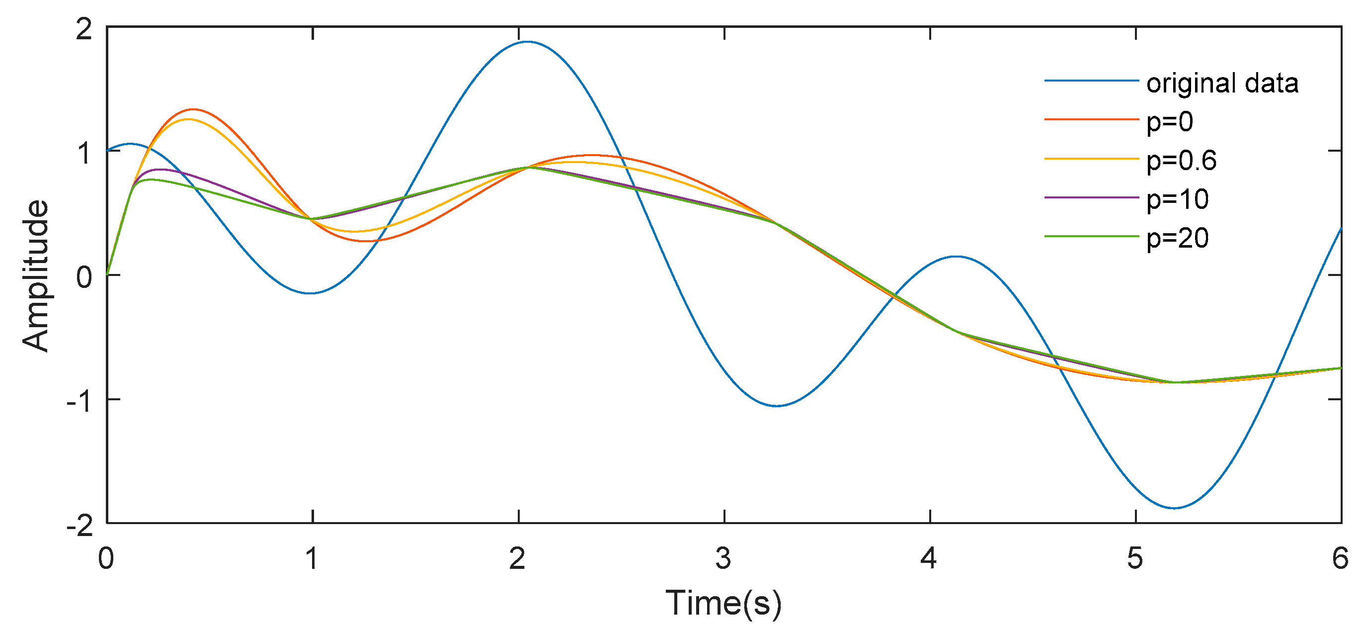
3.1. Rational Spline Interpolation

Since the piecewise linear transformation lacks enough smoothness, a new alternative interpolation method named rational spline interpolation is introduced in this paper. When using the rational spline interpolation, the shape of the fitting curve will change as the pole parameter p varies. Hence, it is easy for us to determine which curve is more suitable to fit the discrete points. Here the definition of rational spline interpolation function is outlined in some detail [24].

Definition 1.

Given a node sequencex_i (i = 1, 2, …) in interval [a, b] and the corresponding function values are y_i (i = 1, 2, …). The rational spline function s(x) satisfies: (1) s(x_i) = y_i, i = 1, 2, …, n, (2) has continuous second derivative in interval [a, b].

Then in the fragment interval [x_i, x_i+1] (i = 1, 2, …, n − 1), the rational spline can be described as follows:

s_i(x) = A_iu + B_it + C_iu³/(1 + pt) + D_it³/(1 + pu), p ≥ −1

(5)

where t = (x − x_i)/h_i = (x − x_i)/ (x_i+1 − x_i), u = 1 − t. In Formula (5), p is the pole parameter used to control the degree of tightness of the spline curve. A_i, B_i, C_i and D_i are the coefficients that make s(x) have continuous first and second derivatives, which can be described as the second derivative value at the node:

C_i = y_i″h_i/q,

(6)

D_i = y_i+1″h_i/q,

(7)

A_i = y_i − C_i,

(8)

B_i = y_i+1 − D_i

(9)

Definition 2.

The second derivative at the node can be obtained by the following linear equations:

h_i−1y_i−1″/(h_i−1 + h_i) + (2 + p)y_i″ + h_iy_i+1″/(h_i−1 + h_i) = q(d_i − d_i−1)/(h_i−1 + h_i),i = 2, 3, …, n − 1

(10)

where, d_i = (y_i+1 − y_i)/h_i, q = 2(p² + 3p + 3). Equation set (10) contains n − 2 equations, plus boundary conditions s″(x₁) = m₁ and s″(x_n) = m_n, can form a system of n linear equations with n unknowns. When p ≥ −1, the system of equations is a strictly diagonally dominant matric, and y_i″ (i = 1, 2, …, n) can be solved by chasing method. Then the results of A_i, B_i, C_i, D_i, and s_i(x) in the interval [x_i, x_i+1] can be obtained by taking y_i″ into Formulas (6)–(9).

From Formula (5), it can be seen that the pole parameter p can control the shape of the spline curve s(x). When p = −1, s(x) becomes a quadratic spline function showed relatively larger volatility and generally did not apply to strive for fitted curve of discrete points; when p = 0, q = 6, it can be seen from Equation (10) that s(x) is a cubic spline function, so the cubic spline function is a special case of the rational spline function. In addition, as p increases, the last two terms of Formula (5) will gradually decrease, and s(x) will continue to tighten. Furthermore, when p tends to infinity, the last two terms of Formula (5) will become zero, and s(x) will become a piecewise linear interpolation function. Therefore, the piecewise linear transform is also a special case of rational spline interpolation. From the above, we can know that, by adjusting the pole parameter p, the desired fitting curve shape can be obtained theoretically, and the decomposition error can be reduced.

The shape of the local mean curve can be changed by adjusting the pole parameter p, as shown in Figure 4. It can be seen that with the change of p, the degree of tightness and smoothness of the local mean curve has also changed accordingly. Thus, the result and precision of subsequent decomposition will be affected.

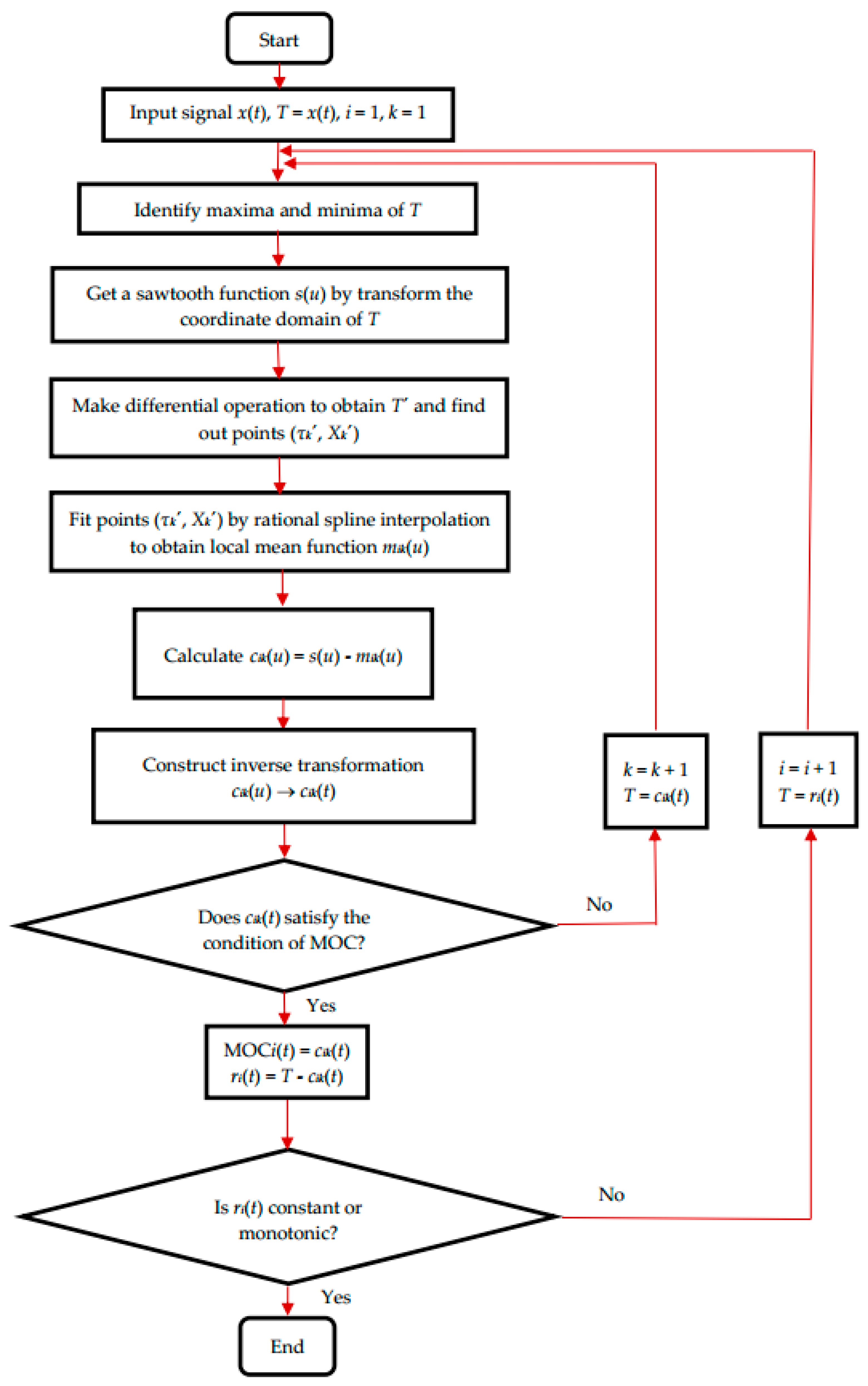
3.2. Rational Spline Based-LOD Method

Based on the above discussion about the interpolation method, it is not difficult for us to conclude that rational spline interpolation is available for precisely fitting discrete points. Furthermore, the mean function algorithm plays a crucial role in the decomposing results with respect to LOD. Hence, the rational spline-based LOD method (RS-LOD) is proposed in this paper. For a given a signal x(t), the algorithmic procedure of the RS-LOD can be described as follows:

(i) Finding out all local extrema X_k, k = 1, 2, …, M and corresponding time values τ_k, k = 1, 2, …, M of original signal x(t). In order to reduce the decomposed error, the function with respect to coordinate domain transform is defined by performing a transformation from original data domain coordinate (t, x) into sawtooth domain coordinate (u, s). The transformation formula can be expressed as:

$$u\left(t\right)={\tau }_k+\left(x\right(t)-X_k)(t-{\tau }_k)/(X_{k+1}-X_k),t\in [{\tau }_k,{\tau }_{k+1}),k=1,2,\dots ,\mathrm{M}$$

(11)

s(u) = x(t),

(12)

From the Formulas (11) and (12), we can see that the coordinate transformation does not change the amplitude of the signal (the direction of ordinate), but only compresses or expands the time axis (the direction of abscissa). Hence, the data point density of different signal positions can be changed without changing the amount of data, and thus to highlight the local characteristic information.

(ii) Making a differential operation for the original signal x(t) to get x′(t) and finding out the time values τ_k′, k = 1, 2, …, N corresponding to the extrema of x′(t). At the same time, finding out function values X_k′, k = 1, 2, …, N corresponding to the time values τ_k′ in original signal x(t). Then the local mean function m₁(u) can be derived by using rational spline function to fit the (τ_k′, X_k′) in sawtooth domain.

(iii) Subtract the local mean function m₁(u) from the sawtooth domain function s(u) of the original signal, and then the high-frequency oscillatory function c₁(u) can be obtained:

c₁(u) = s(u) − m₁(u),

(13)

(iv) Restore the coordinates of c₁(u) from the sawtooth domain to the original data domain c₁(t) using the inverse transformation. The inverse transformation formula can be written as:

$$t\left(u\right)={{\tau }_k}^{\prime }+(X_{k+1}-X_k)(u-{{\tau }_k}^{\prime })/\left(x\right(t)-X_k),u\in [{{\tau }_k}^{\prime },{{\tau }_{k+1}}^{\prime }),k=1,2,\dots ,\mathrm{N}-1$$

(14)

$$c_1\left(t\right)=c_1\left({{\tau }_k}^{\prime }\right)+\left(c_1\right(u)-c_1({{\tau }_k}^{\prime }\left)\right)({{\tau }_{k+1}}^{\prime }-{{\tau }_k}^{\prime })/(t-{{\tau }_k}^{\prime }),t\in [{{\tau }_k}^{\prime },{{\tau }_{k+1}}^{\prime }),k=1,2,\dots ,\mathrm{N}-1$$

(15)

Ideally, c₁(t) is the first component MOC₁(t) of original signal x(t) when c₁(t) is a mono-component signal of instantaneous frequency with physical meaning.

(v) If c₁(t) is not a mono-component signal of the instantaneous frequency with a physical meaning, we should repeat the above procedure m times until c_m(t) is a mono-component signal of instantaneous frequency with physical meaning. In other words, in this situation, c_m(t) will be the first component MOC₁(t) of the original signal.

(vi) This derived MOC₁(t) is then subtracted from the original signal x(t), obtaining a new function r₁(t). Regard r₁(t) as a new original signal and repeat the procedure (i)~(v) n times until r_n(t) is a monotonic function. Thus, x(t) may be decomposed into the sum of n MOCs and residue r_n(t). i.e.,

$$x(t)={\sum }_{i=1}^n{\mathrm{MOC}}_i\left(t\right)+r_n(t),$$

(16)

The flowchart of the RS-LOD method is illustrated in Figure 5.

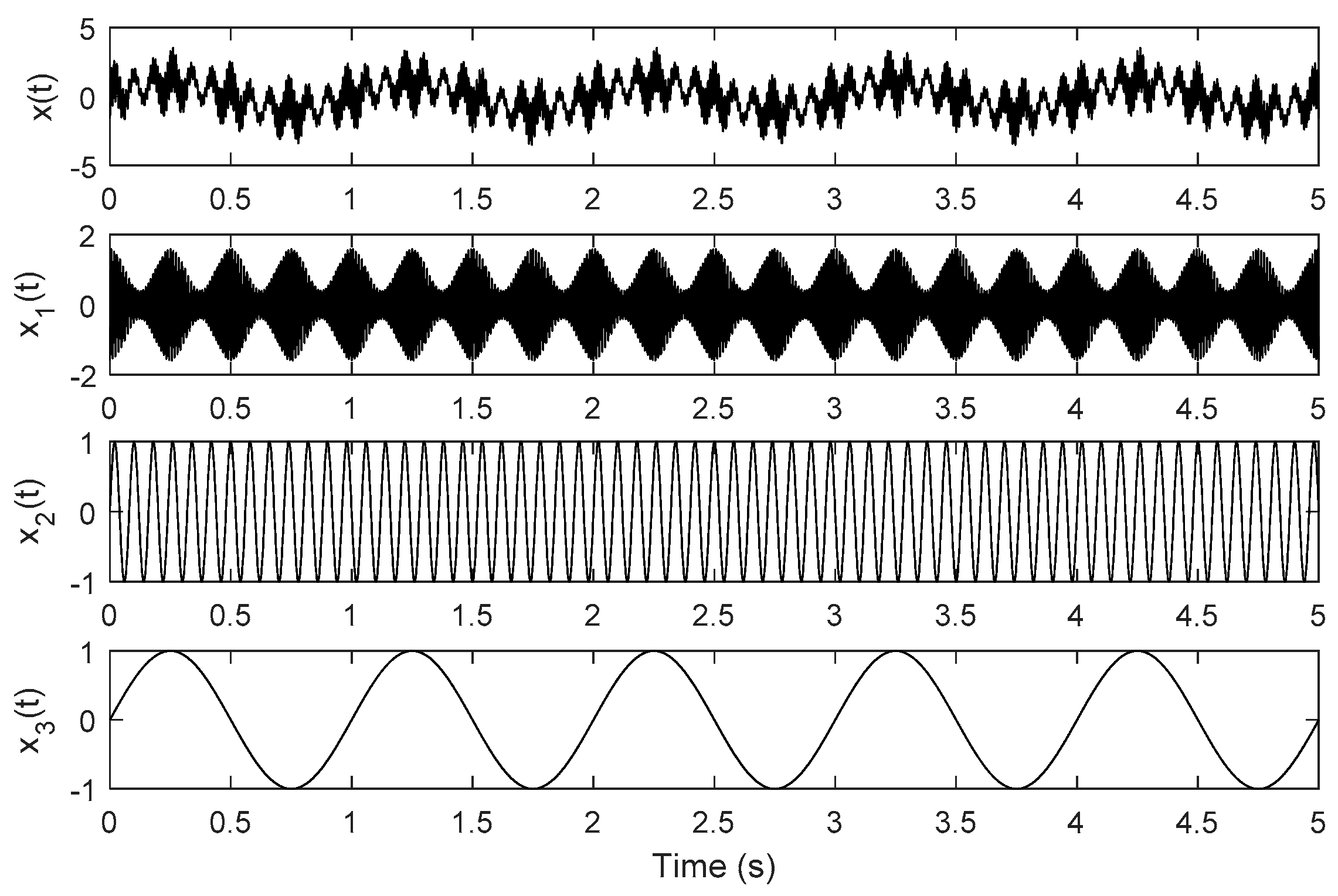
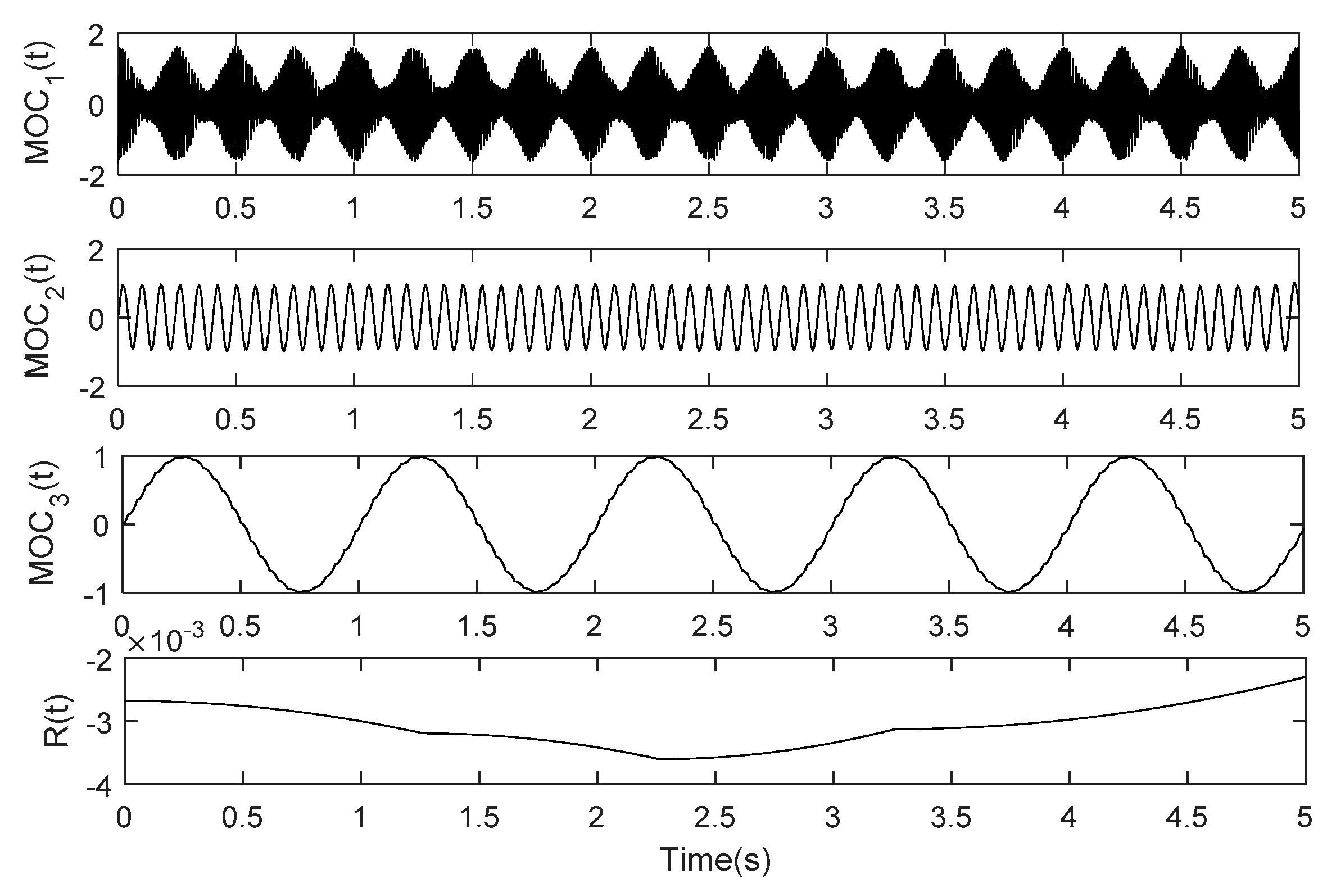
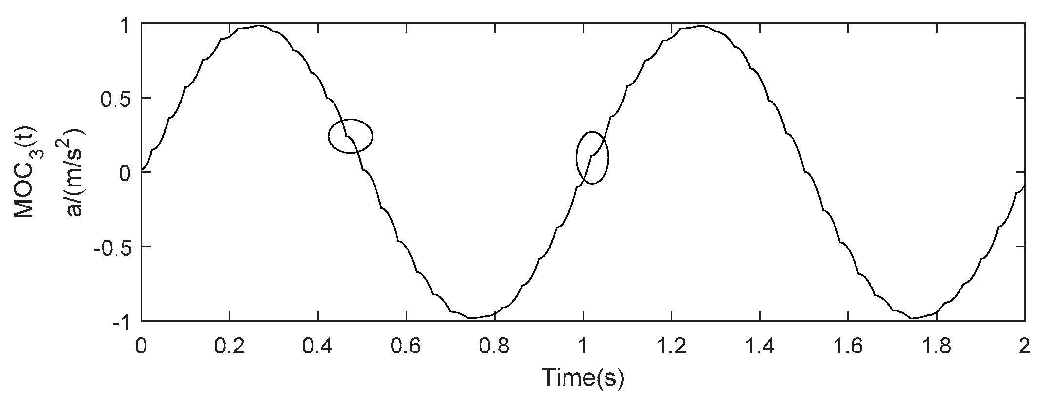
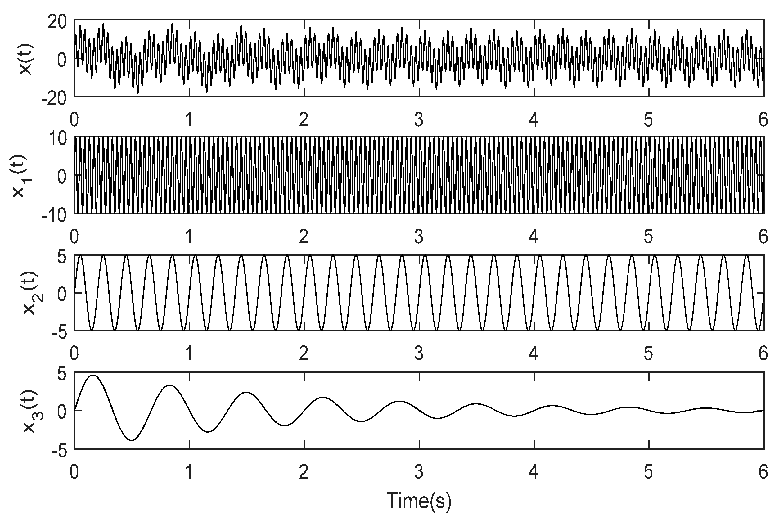
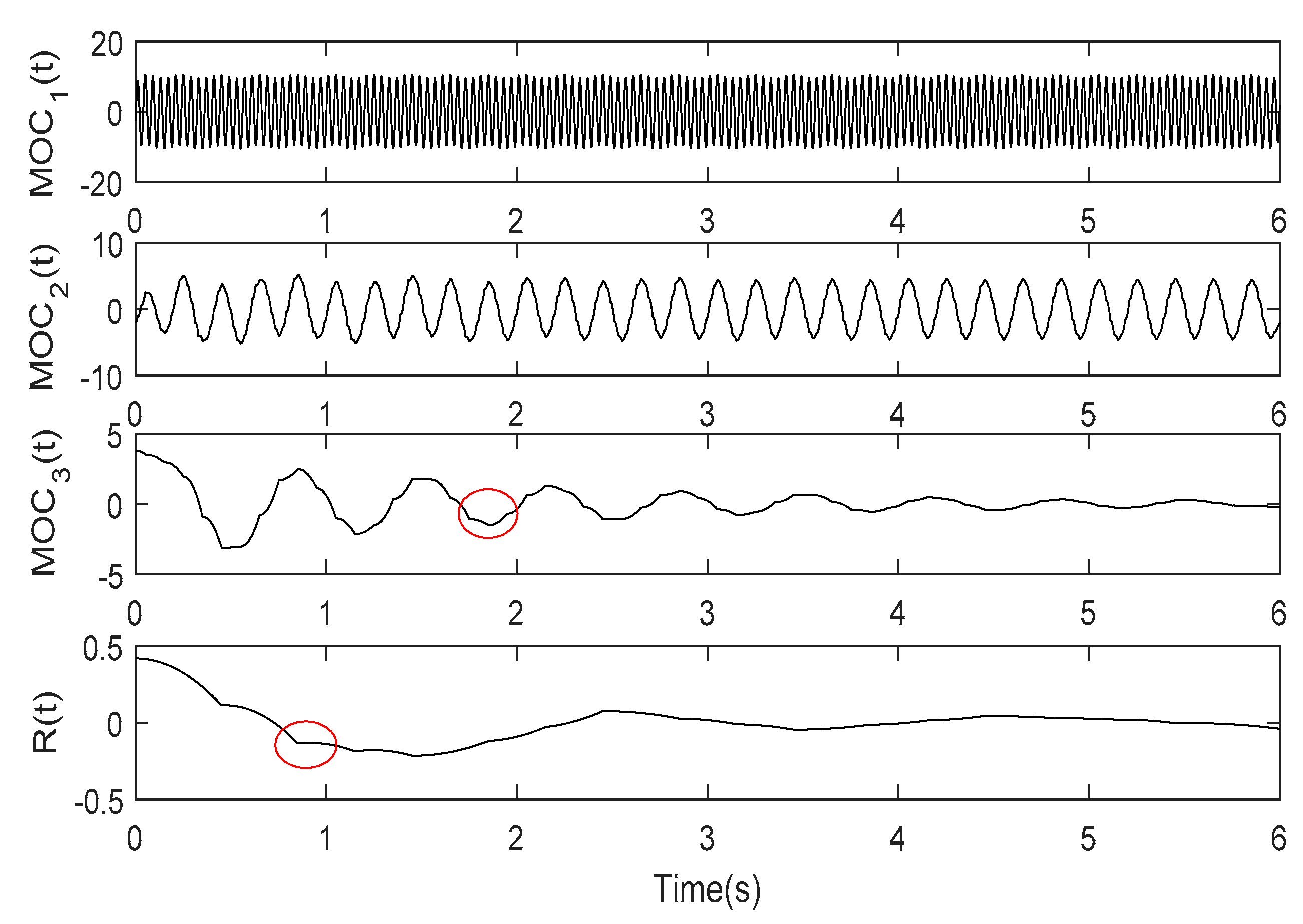
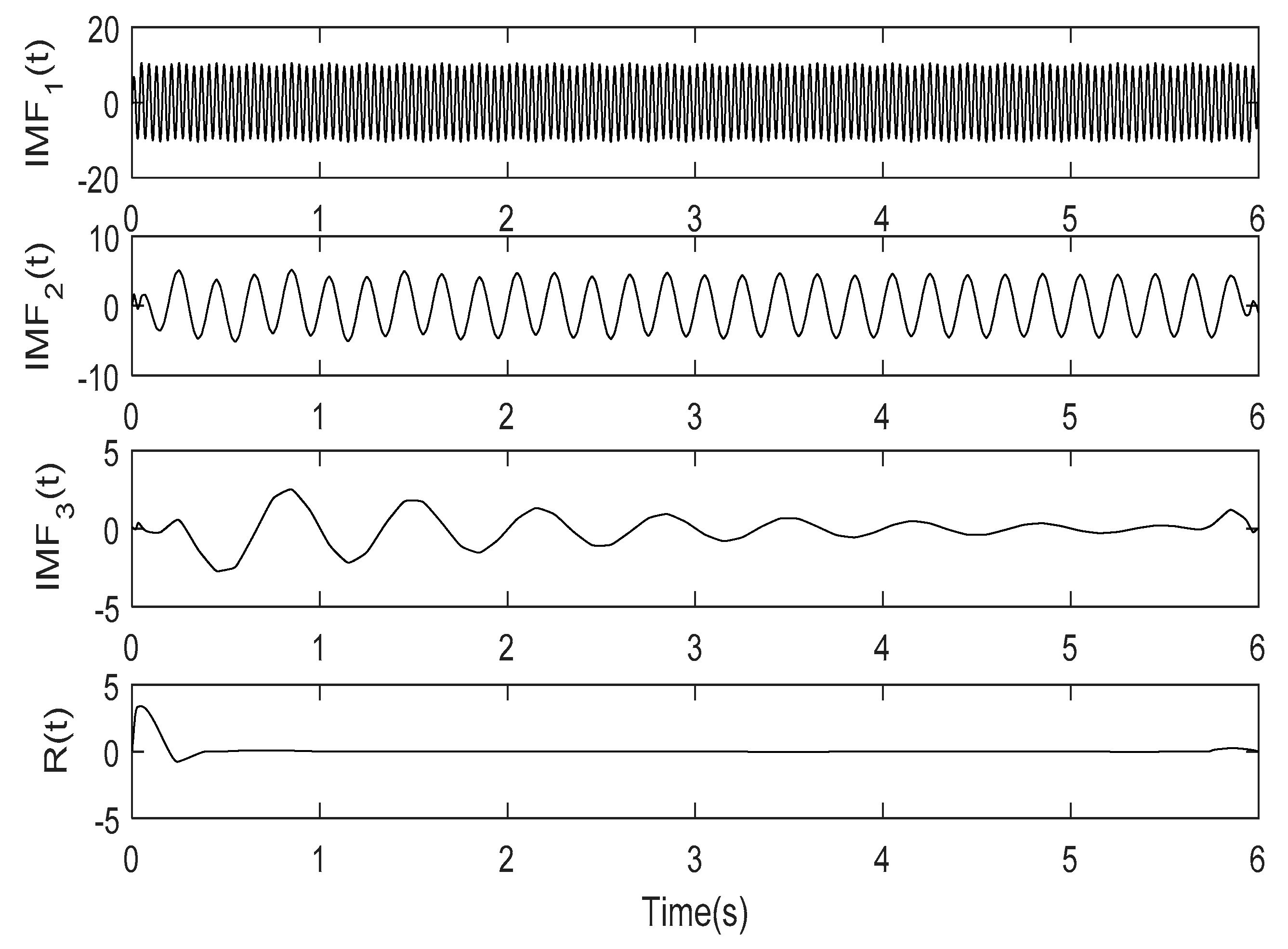
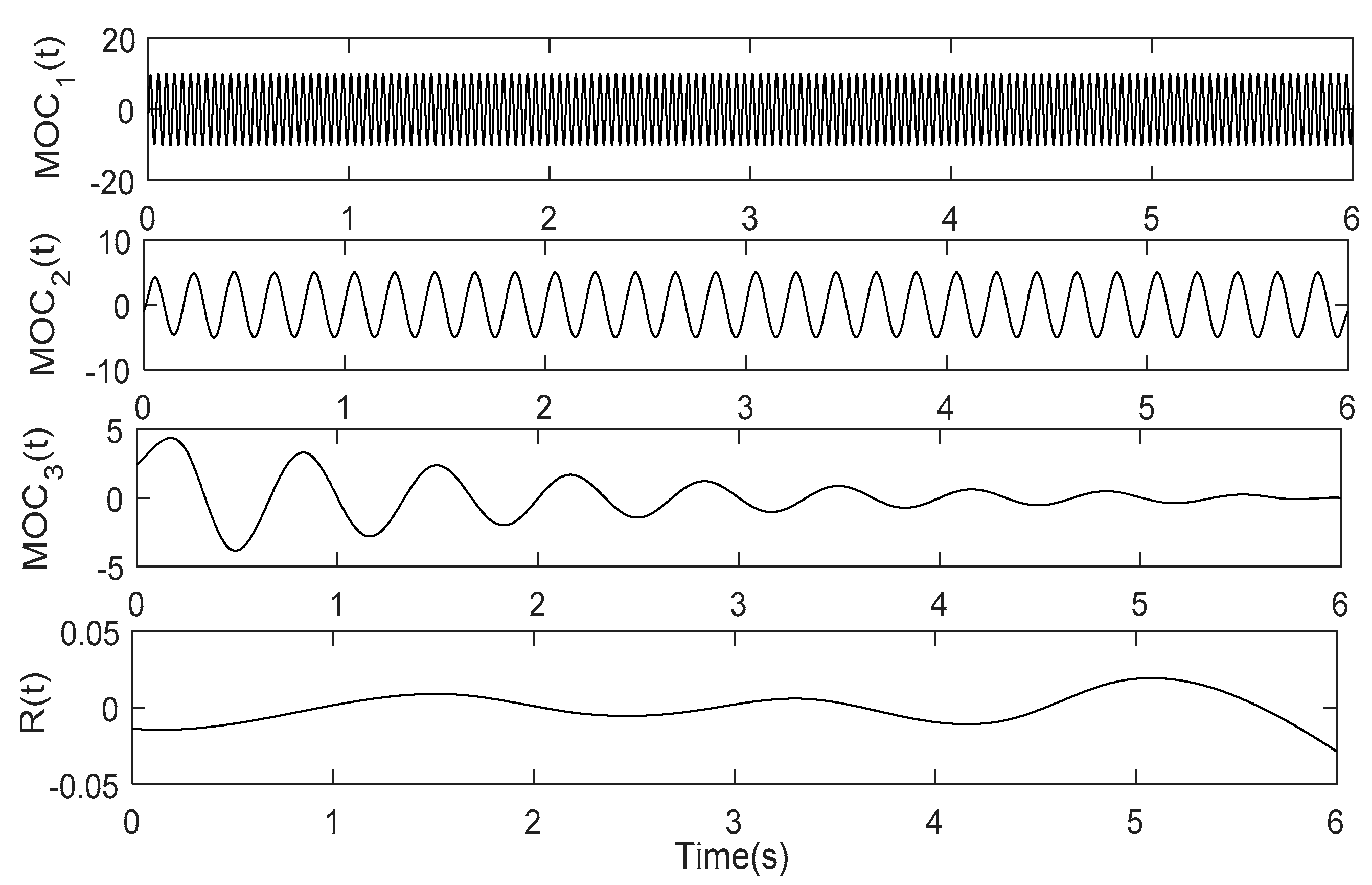
4. Application to Simulation Signal

In order to verify the effectiveness of the RS-LOD method and compare it with other methods, the same simulation signal is analyzed using RS-LOD, EMD, and LOD methods, respectively. In a comparison of the analysis processing, the end effects are not solved. It is to say that end effects may appear in all methods. Therefore, the severity of end effects can be used as an assessing index to compare the three methods. Additionally, the standard deviation (SD) criterion [7] is adopted as the iterative stopping condition, that is, by calculating the standard deviation of the results of two consecutive iterations, and comparing with the predetermined threshold to determine the iterative termination. The predetermined threshold is 0.5 in this paper.

Here we consider a multi-component AM-FM simulation signal x(t):

x₁(t) = 10sin(50πt),

(17)

x₂(t) = 5 sin(10πt),

(18)

x₃(t) = 5exp(−0.5t) sin(3πt),

(19)

x(t) = x₁(t) + x₂(t) + x₃(t),

(20)

where t $\in$ [0, 6], the setting sampling frequency 1000 Hz, and the simulation signal consists of a modulated signal and two sine signals. The time-domain waveforms of x(t) and its three components x₁(t), x₂(t), and x₃(t) are shown in Figure 6.

The simulation signal x(t) is decomposed by using the LOD, EMD, and RS-LOD method and the decomposition results are presented in Figure 7, Figure 8 and Figure 9, respectively. It can be seen from Figure 7, Figure 8 and Figure 9 that all three methods can decompose the original signal from high frequency to low frequency in turn, and the decomposed three components correspond to the x₁(t), x₂(t), and x₃(t) of the original signal, respectively. However, it is also obvious found that there exist some differences in the results of their decomposition. In Figure 7, the decomposition result of the LOD is serrated, and the smoothness is poor (marked by a red circle). The RS-LOD decomposition result shown in Figure 9 (set p = 5) does not show this phenomenon, and because of the good smoothness, the cumulative error is small; thus the amplitude of the residue is obviously smaller than that of LOD. In Figure 8, due to the cubic spline function used by EMD, the end effects are obvious [20], and the amplitude of residue is also larger than that of RS-LOD because of the error of the end effects. In summary, we can see that the decomposition result of the RS-LOD is better than that of LOD and EMD as a whole.

In addition, in order to quantitatively compare the decomposition results of the three methods, the assessing indicators, including the index of orthogonality (IO) [7], the number of sifting times, and the consuming time are used to evaluate the results. The three algorithms have been run 30 times using MATLAB R2017b to above simulation signal x(t) on the same computer, respectively, and all using SD < 0.5 as iterative stopping condition. The average values of three assessing indicators are calculated and counted, and the results are shown in

Table 1. Three assessing indicators for comparison among EMD, LOD, and RS-LOD methods.

Method	Number of Sifting Times	IO	Consuming Time(s)
EMD	38	0.0834	4.0328
LOD	27	0.0574	0.0381
RS-LOD	30	0.0347	1.3226

.

It can be seen from Table 1, the IO value, which reflects the decomposition effects, the RS-LOD is the best of the three. Comparing the LOD method which uses linear transformation completely, the consuming time of the RS-LOD is a little longer, but they are both obviously shorter than that of the EMD method. Therefore, through a quantitative comparison, the RS-LOD method also has some advantages in terms of decomposition effects and computational efficiency.

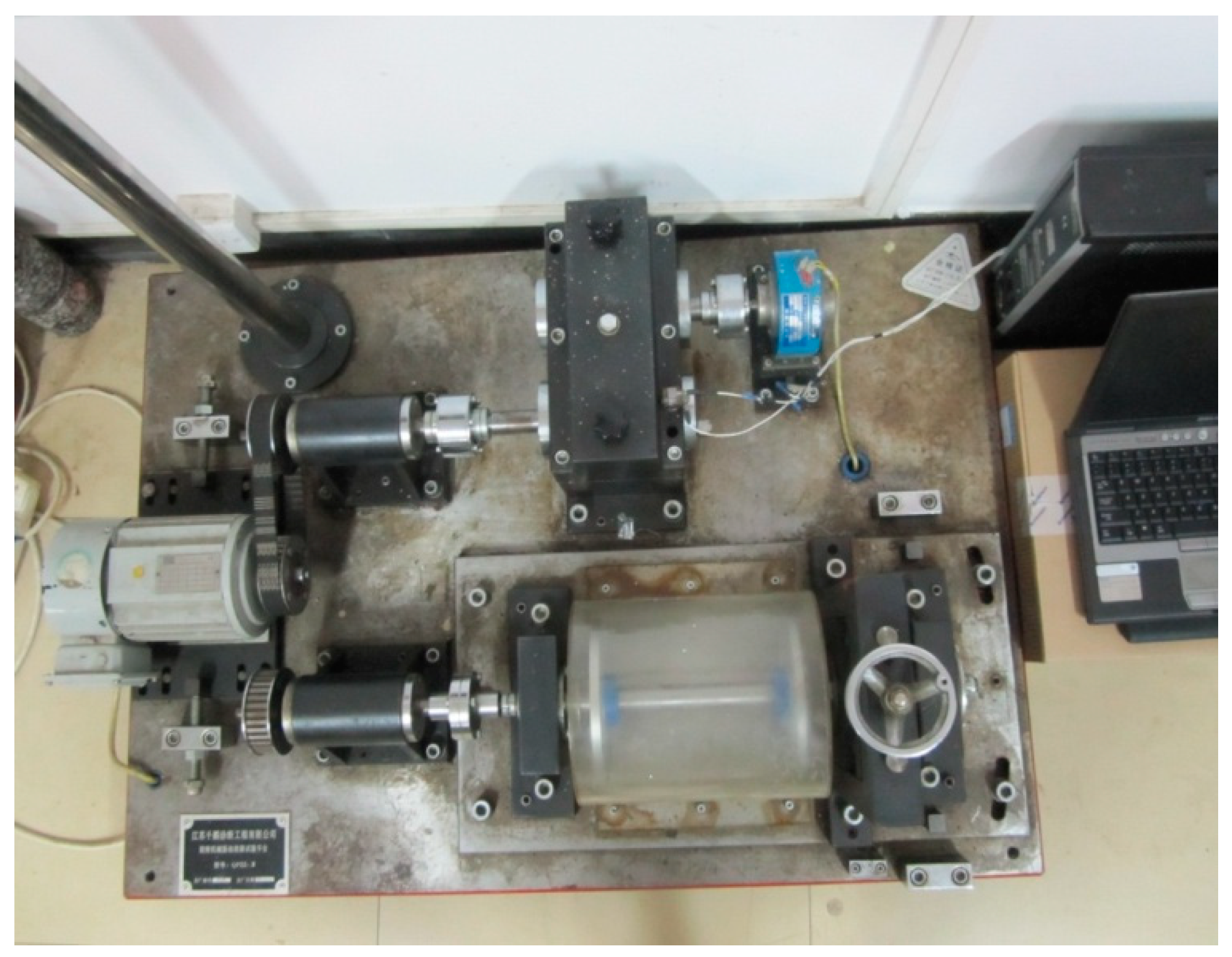
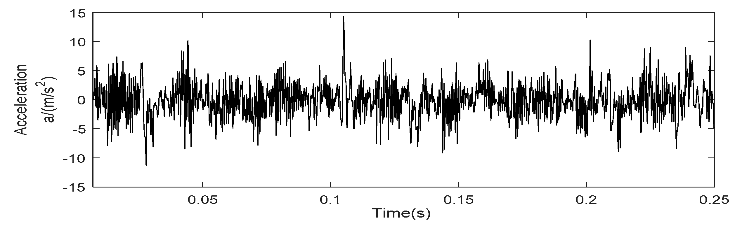
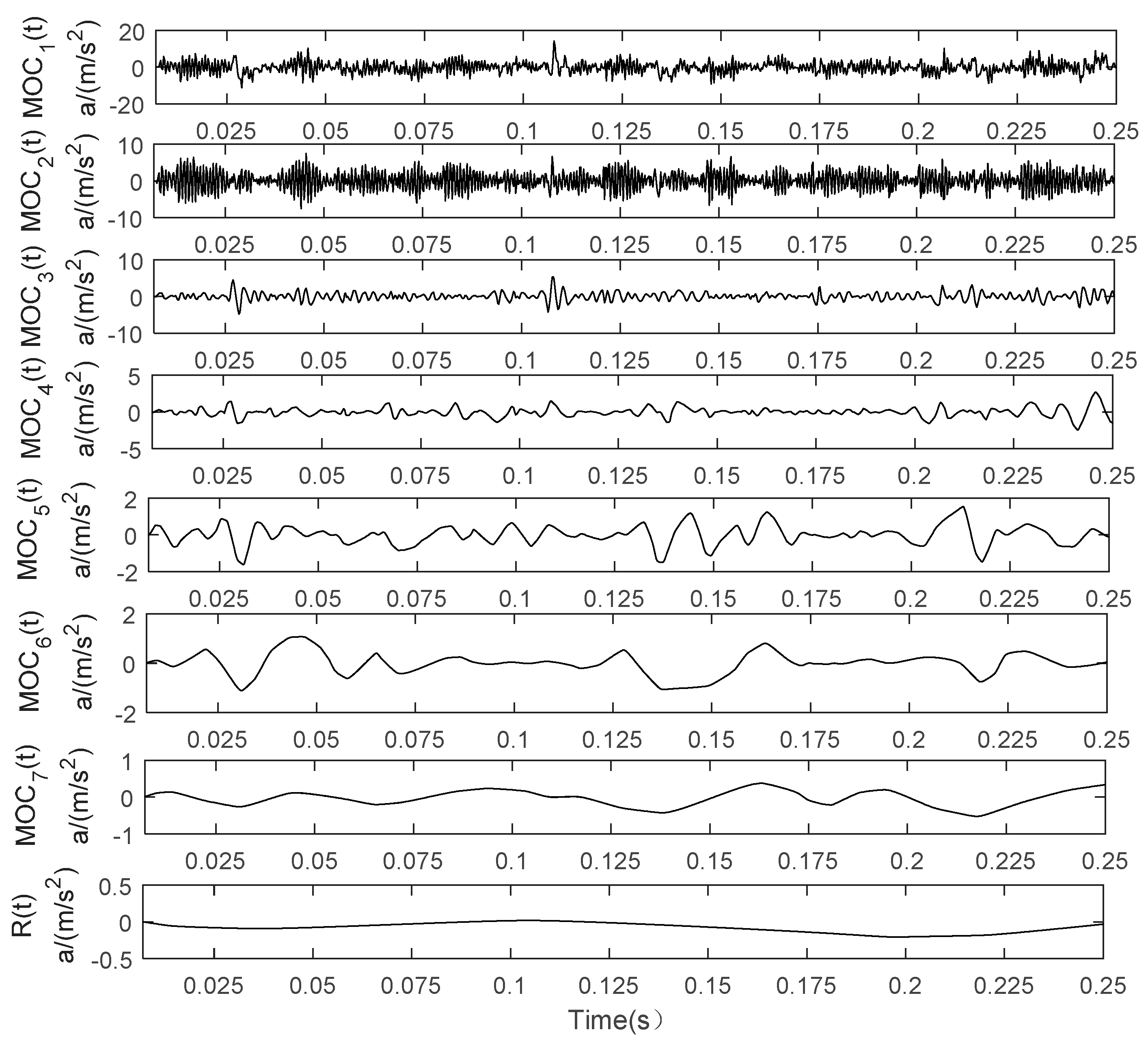
5. Application to Rotating Machinery Fault Diagnosis

When gear or rolling bearing is operated with local faulty, the measured vibration signal generally is a multi-component AM-FM signal, and the high-frequency vibration components, such as natural frequency vibration and mesh frequency vibration, are modulated by shock pulse caused by local faults [27,28]. The RS-LOD method can decompose the multi-component AM-FM signal into a series of single-component signals, while performing the Hilbert transform on each single-component signal can obtain an envelope signal with a physical meaning. Theoretically, the modulation information caused by fault can be extracted from the spectrum of these envelope signals. Therefore, RS-LOD is very suitable for extracting characteristic information from fault vibration signals of the rolling bearing and gear.

The main steps of extracting fault characteristics based on the RS-LOD method can be summarized as follows: Firstly, the vibration signal is decomposed into a serious of the MOC components by RS-LOD method. Secondly, the envelope signal of MOC component with fault characteristics is obtained by the Hilbert transform. Finally, the frequency spectrum of the envelope signal is analyzed for effectively extracting the fault characteristic frequency.

5.1. Application to Rolling Bearing Fault Diagnosis

In order to verify the proposed method, the rolling bearing failure experiment was carried out on a rotating machinery fault test bench. The top view of the experimental device is shown in Figure 10. The adjustable speed motor in this system is a DC servo motor with a power of 600 W. The rolling bearings are installed on four bearing chocks, and both driving gear and driven gear are spur gears. The moment of the inertia of the load is 0.03 kg·m². In this experiment, the tested bearing is the 6311-type rolling bearing, which was formed the inner-race and outer-race faults by laser cutting technology, and the slot width and depth are 0.15 mm and 0.13 mm, respectively. The vibration signals are collected by two piezoelectric acceleration transducers, which are horizontally and vertically fixed to the bearing housing. Figure 11 shows the time-domain waveform of vibration acceleration signal of the rolling bearing with outer-race fault. The sampling frequency is 4096 Hz, and the rotating frequency is f_r = 25 Hz, and by calculating the outer-race fault characteristic frequency is f_o = 76 Hz.

The vibration signal shown in Figure 11 is decomposed by the RS-LOD method. The value of the pole parameter p will affect decomposition results and decomposition time; therefore, we need to determine the value of p firstly.

Table 2. The number of sifts versus the different values of the pole parameter p.

p	MOC1(t)	MOC2(t)	MOC3(t)	MOC4(t)	MOC5(t)	MOC6(t)	MOC7(t)	MOC8(t)	Total
0	5	7	6	7	-	-	-	-	25
0.5	5	6	6	8	8	-	-	-	33
1	5	7	6	7	8	8	-	-	41
2	5	7	6	6	8	7	-	-	39
5	5	7	6	6	8	7	8	-	47
10	5	7	7	6	7	7	7	-	46
20	5	7	8	8	8	8	7	8	59
50	5	7	8	7	7	8	8	8	58

shows the number of sifts required to identify each MOC. It can be seen that the number of sifts required for each MOC component and the total number of sifts for per decomposition for a range of p values. When p takes relatively smaller value at a certain range, the total number of sifts required is less, and the number of MOCs obtained is also less. From these two standards, when p takes the range of 0 to 10, it is possible to get higher decomposition efficiency.

Table 3. Index of orthogonality (IO) and consuming time versus different values of pole parameter p.

p	0	0.5	1	2	5	10	20	50
IO	0.1990	0.1846	0.1725	0.1408	0.1192	0.0140	0.0135	0.0132
Consuming time(s)	0.4792	0.4501	0.4799	0.5264	0.6810	0.5438	0.7909	0.9873

lists the IO value and decomposition time for different p values. It can be seen that with the increase of p, the IO value decreases gradually, and the decomposition time increases during the fluctuation. However, when p is greater than 10, the decrease of IO value is not obvious and undergoes gradual stabilization, but the decomposition time increases obviously. Therefore, consider the decomposition effects and decomposition time to determine the p value is 10 in this decomposition.

When p = 10, the decomposition results are shown in Figure 12, and the high-frequency components MOC₁(t) and MOC₂(t) are shown in Figure 13. It can be seen that seven MOC components and one residue are obtained from high-frequency to low-frequency, and the decomposition effects are ideal. According to the rolling bearing fault vibration mechanism, the fault vibration signal of the rolling bearing is the modulation signal with the natural frequency of a rolling bearing system as the carrier frequency and the fault characteristic frequency as the modulation frequency. Therefore, the working condition of the rolling bearing can be judged by the envelope spectrum of the fault vibration signal. Additionally, the natural frequency of the rolling bearing system usually exists in the high-frequency components. Hence, by applying the Hilbert transform to the MOC₁(t), and the obtained Hilbert envelope spectrum, as shown in Figure 14, it can be easily seen that, except for the spectral line of rotating frequency (25 Hz), there are also obvious spectral lines of the outer-race fault characteristic frequency (76 Hz) and its double (152 Hz) can be found in the Hilbert envelope spectrum. Therefore, the fault of the outer race of the rolling bearing can be judged, which is consistent with the actual situation, and shows the effectiveness of the proposed method.

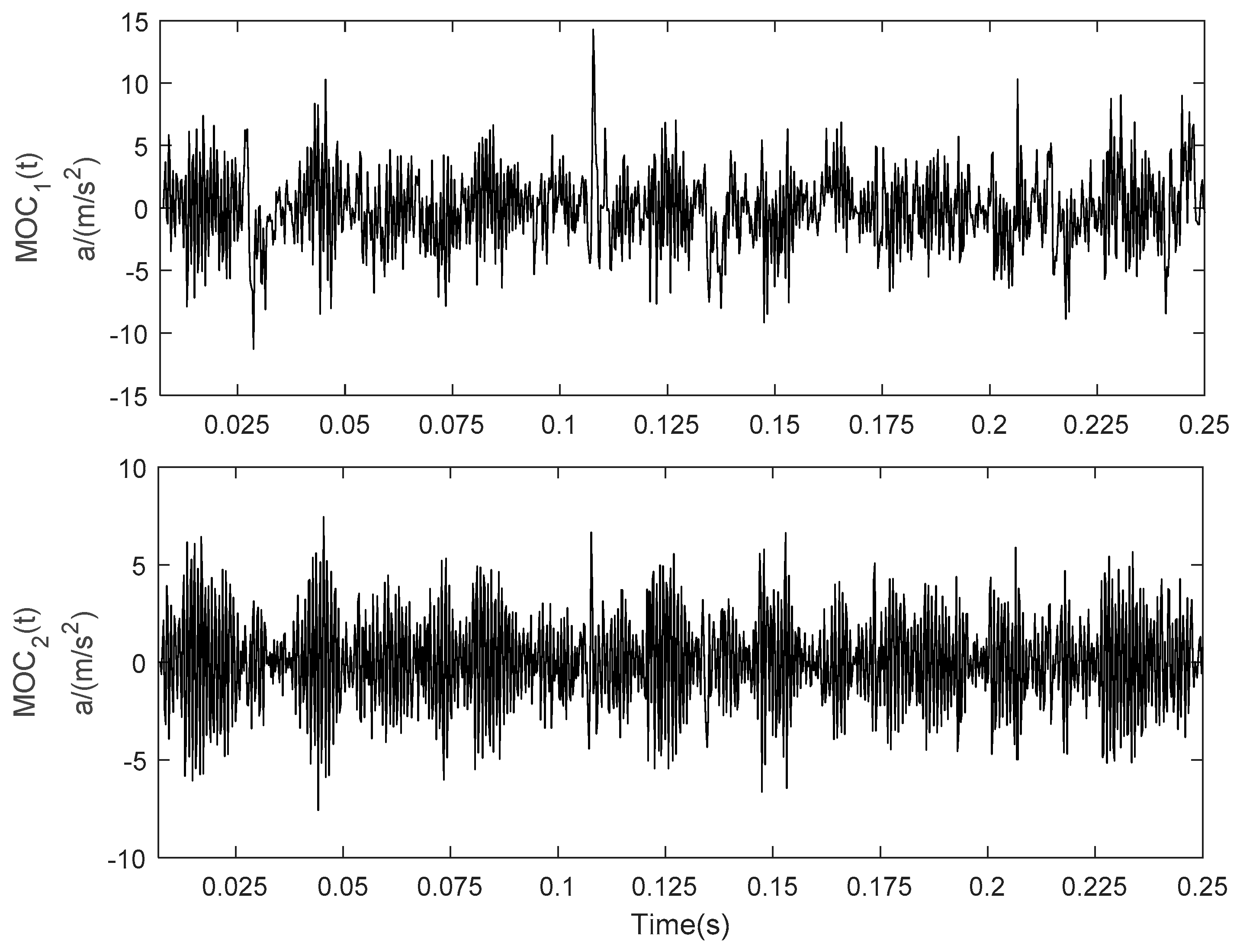
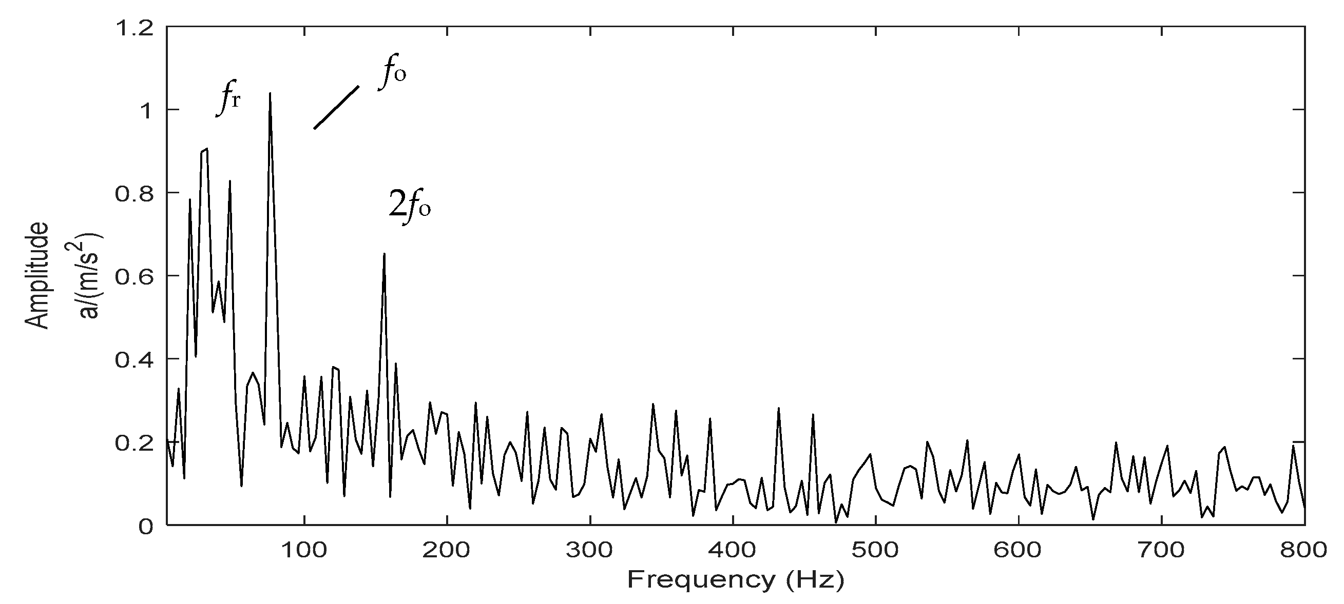
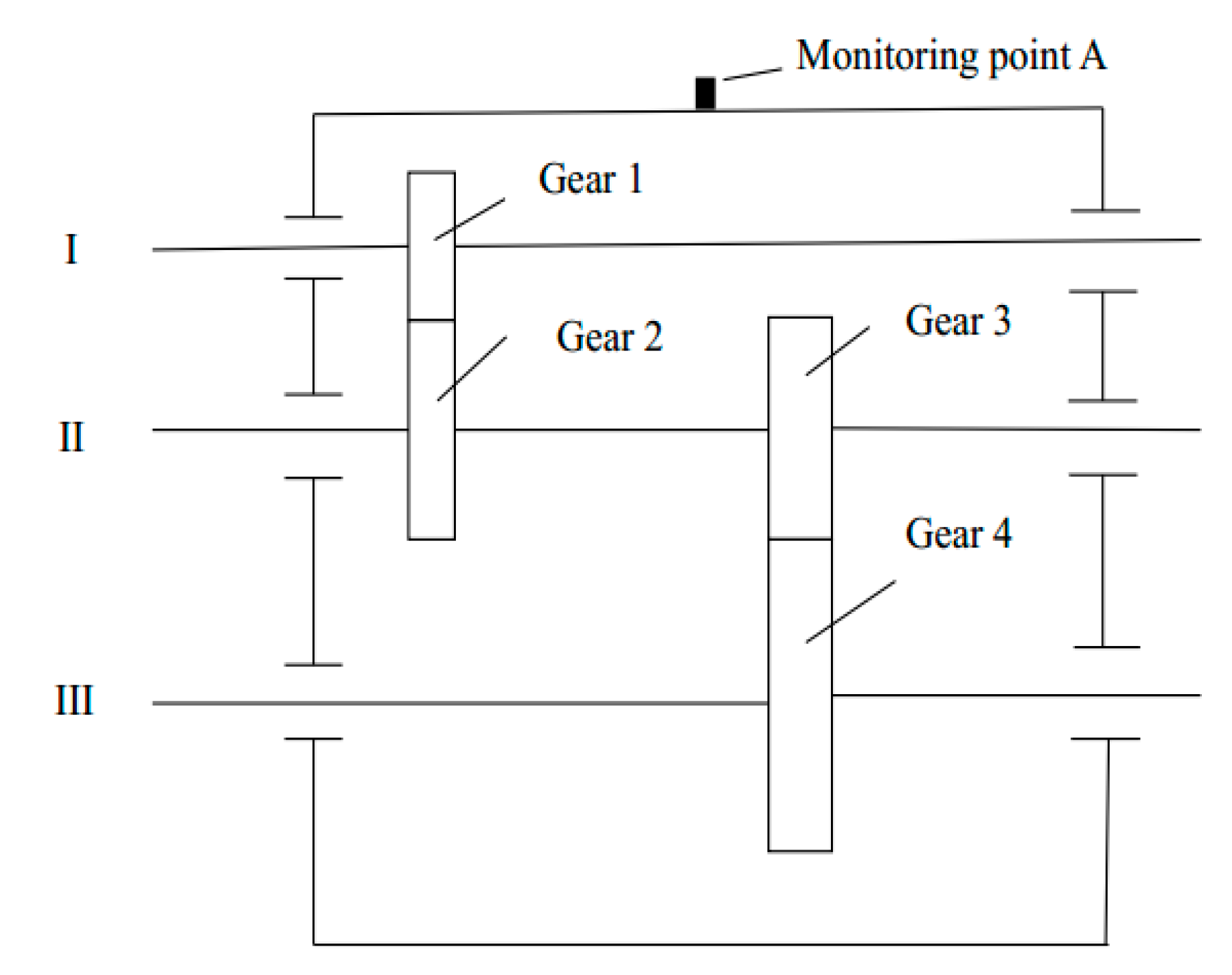
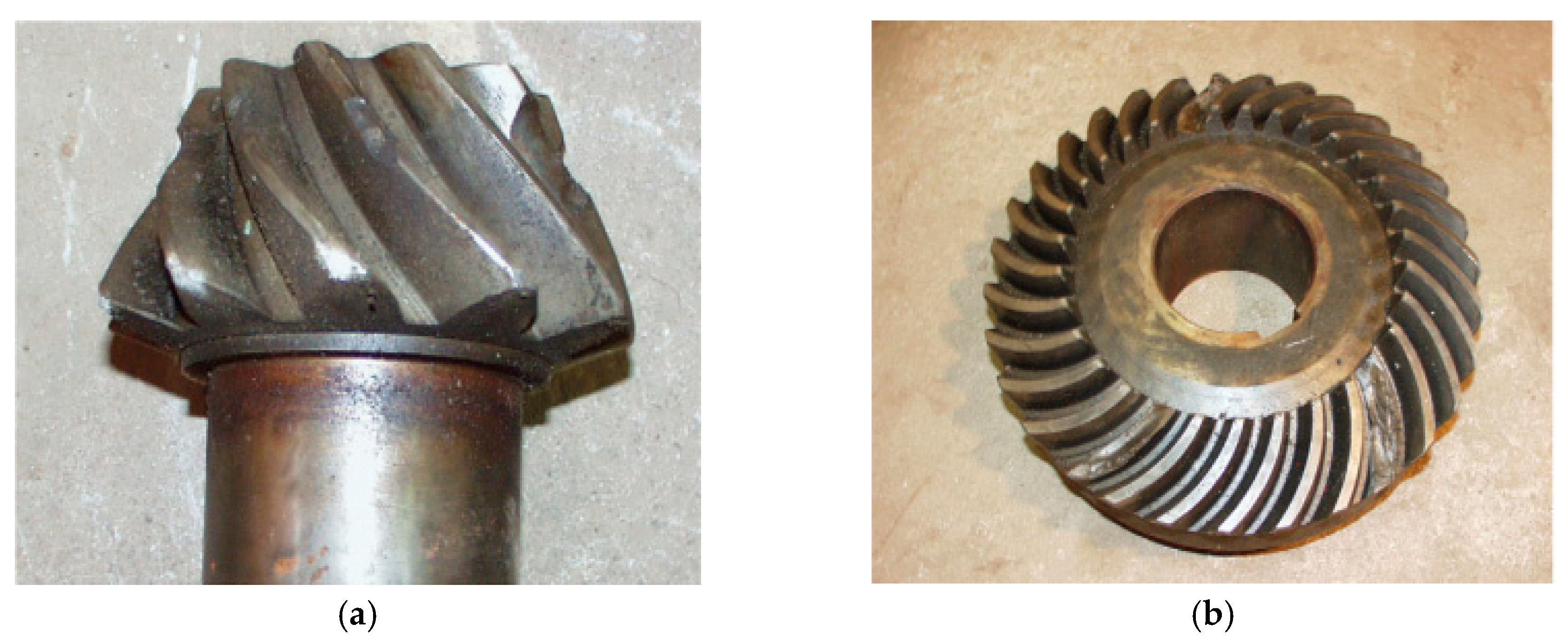
5.2. Application to Fan Gearbox Fault Diagnosis

Figure 15 shows the structure of the No.3 fan gearbox of a petrochemical company, in which the teeth number of gears 1, 2, 3, and 4 are 11, 31, 23, and 53, respectively. The rotational speed of shaft I is n_I = 980 r/min, namely, the rotating frequency of shaft I is about f_I = 16.3 Hz, the rotating frequency of shaft II is about f_II = 5.8 Hz, and the rotating frequency of shaft III is about f_III = 2.5 Hz. One day, the online monitoring system found that the vibration of the no.3 fan gearbox was abnormal. The root means square value of the vibration acceleration signal (on monitoring point A shown in Figure 15) was relatively bigger than the threshold value, but the fan running was not affected, and the date was close to the normal shutdown maintenance date, so keep observation. During the subsequent shutdown maintenance, the fan gearbox was examined. It was found that four gears of gearbox had different degrees of wear and tooth surface glue, especially the wear of gear 1 and gear 2 were very serious, which can be shown in Figure 16.

In order to verify that Hilbert envelope spectrum based on RS-LOD can accurately identify the fault condition of the gearbox, a vibration acceleration signal (the sampling frequency is 1024 Hz) measured on the same day is selected for analysis, and which time-domain waveform and amplitude spectrum are as shown in Figure 17 and Figure 18. By preliminary analysis, the main frequency components include the mesh frequency of gear 1 and gear 2, the mesh frequency of gear 3 and gear 4, and many other unknown frequencies. Moreover, the sidebands of the gear mesh frequency are very difficult to distinguish. Therefore, it is hard to estimate whether and where the fault has occurred in the gearbox from the amplitude spectrum in Figure 18. Further, the envelope demodulation technology based on the RS-LOD is used to identify the condition of the gearbox. According to the manner in Section 5.1, we can determine the value of p in this decomposition is 9. A total of ten MOC components are obtained by RS-LOD decomposition, and the first five MOC components are shown in Figure 19. It can be seen that the decomposition effects are good, and there are no obvious distortions. The first three MOC components are further selected for Hilbert envelope analysis, and the results are shown in Figure 20, respectively.

In Figure 20a, it can be seen that there is a spectral line with high amplitude at the double frequency of rotating frequency f_I. In Figure 20b, there are several obvious spectral lines, which at the 1, 2, 3, 4 times of rotating frequency f_I, and at the 1, 2 times of rotating frequency f_II. In Figure 20c. It can be seen at the rotating frequency f_I and 1, 2 times of rotating frequency f_III there are clear spectral lines. According to the distribution and amplitude of above spectral lines, it can be determined that there are certain degree faults in all four gears on three shafts, and the faults on gear 1 and gear 2 are more serious, while the faults on gear 3 and gear 4 are relatively slight. It is consistent with the actual gearbox check, which confirmed the effectiveness of the proposed diagnosis method.

6. Discussion

Through the analysis of simulation signals and experimental signals, we know that the RS-LOD method inherits the strengths of the LOD method, such as fast calculation speed, no obvious end effects, stable decomposition results, and much slighter mode mixing phenomena etc. At the same time, the rational spline function with a pole parameter p is introduced to overcome the problems of MOC component poor smoothness and distortion. For different signals, the optimal local mean curve can be obtained flexibly by adjusting the pole parameter p, reducing the rounding error, and obtaining the optimal component. However, the optimal selection range of pole parameter p of rational spline function is estimated through multiple numerical experiments, i.e., the selection of pole parameter p is subjective and lack of adaptivity. Therefore, how to determine the optimal pole parameter p automatically is a problem that needs further study. In addition, other interpolation methods [29,30] can also be considered to improve the decomposition effects in the future.

7. Conclusions

In order to solve the problems of MOC component poor smoothness and distortion caused by the piecewise linear transformation in the LOD method, the rational spline interpolation is used to replace the piecewise linear transformation and the RS-LOD method is proposed in this paper. Then, the RS-LOD method is used for rotating machinery fault feature extraction. The following conclusions are obtained:

• The analysis of the simulation signal shows that although the consuming time of the RS-LOD method is a little longer than the original LOD method, it solves the problems of MOC component poor smoothness and distortion in the original LOD method, and overall analysis effects are also better than that of EMD and LOD method.
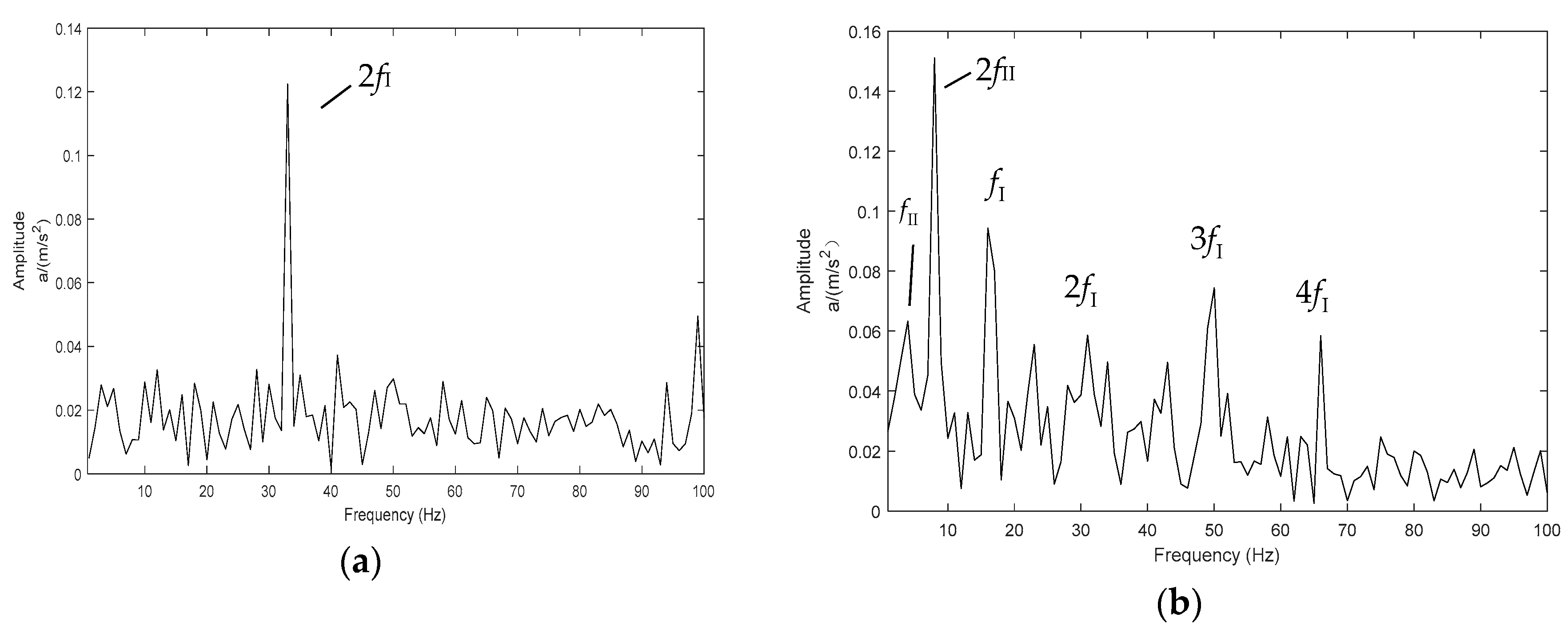
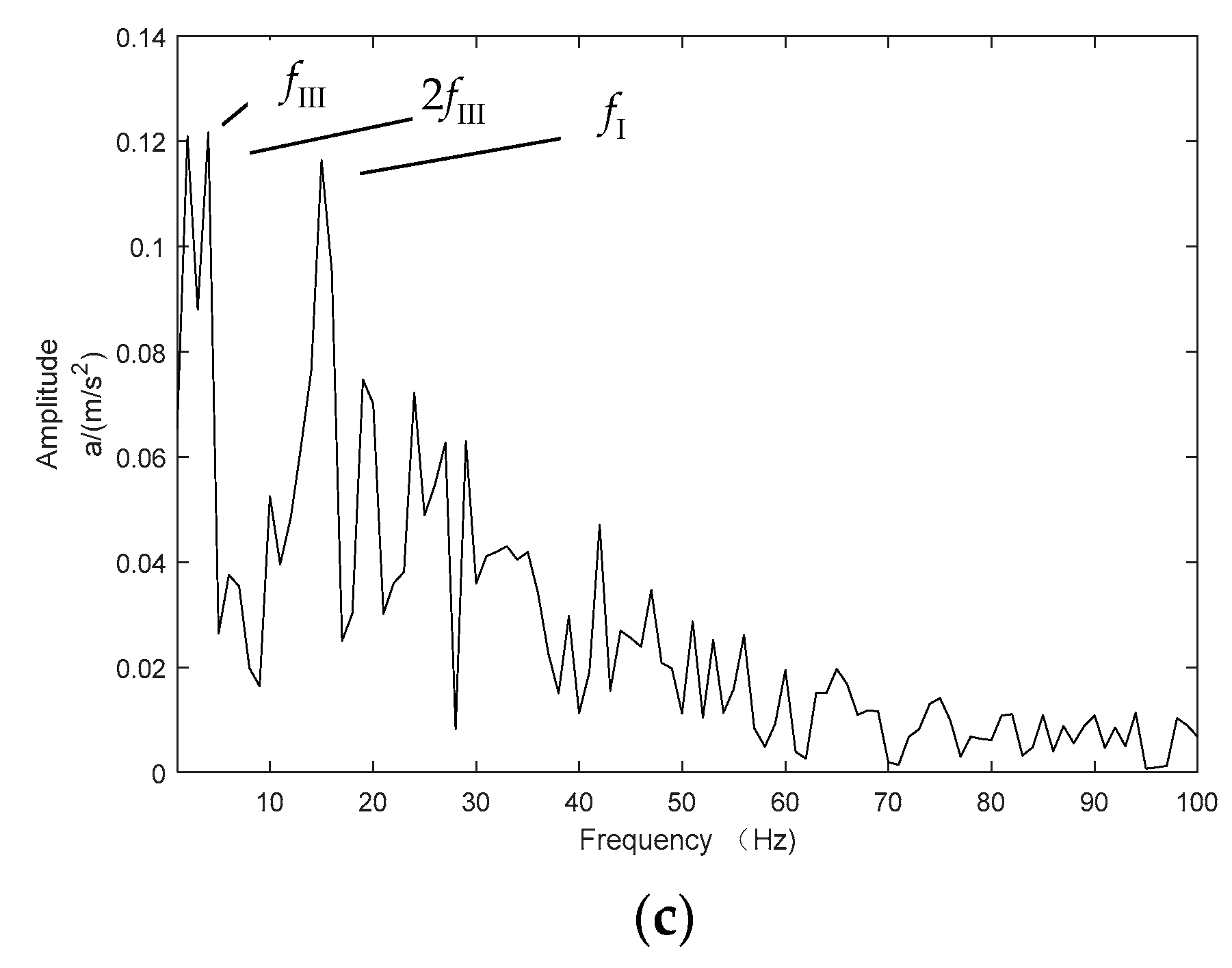
• The analyses of fault vibration signals of rolling bearing and fan gearbox show that the envelope spectrum based on RS-LOD can effectively extract the characteristic fault information of the corresponding vibration signal, which provides a new effective way to extract the vibration signal feature.

References

1. Prudhom, A.; Antonino-Daviu, J.; Razik, H.; Vicente, C.-A. Time-frequency vibration analysis for the detection of motor damages caused by bearing currents. Mech. Syst. Signal Process. 2017, 84, 747–762. [Google Scholar] [CrossRef] [Green Version]
2. Stanković, L.; Mandić, D.; Daković, M.; Brajovića, M. Time-frequency decomposition of multivariate multicomponent signals. Signal Process. 2018, 142, 468–479. [Google Scholar] [CrossRef]
3. Xu, Y.; Zhang, K.; Ma, C.; Li, X.; Zhang, J. An improved empirical wavelet transform and its applications in rolling bearing fault diagnosis. Appl. Sci. 2018, 8, 2352. [Google Scholar] [CrossRef] [Green Version]
4. Dhamande, L.S.; Chaudhari, M.B. Compound gear-bearing fault feature extraction using statistical features based on time-frequency method. Measurement 2018, 125, 63–77. [Google Scholar] [CrossRef]
5. Mateo, C.; Talavera, J.A. Short-time Fourier transform with the window size fixed in the frequency domain. Digit. Signal Process. 2018, 77, 13–21. [Google Scholar] [CrossRef]
6. Yoo, Y.; Baek, J.-G. A novel image feature for the remaining useful lifetime prediction of bearings based on continuous wavelet transform and convolutional neural network. Appl. Sci. 2018, 8, 1102. [Google Scholar] [CrossRef] [Green Version]
7. Huang, N.E.; Shen, Z.; Long, S.R.; Wu, M.C.; Shih, H.H.; Zheng, Q.; Yen, N.C.; Tung, C.C.; Liu, H.H. The empirical mode decomposition and the Hilbert spectrum for nonlinear and non-stationary time series analysis. Proc. R. Soc. A 1998, 454, 903–995. [Google Scholar] [CrossRef]
8. Smith, J.S. The local mean decomposition and its application to EEG perception data. J. R. Soc. Interface 2005, 2, 443–454. [Google Scholar] [CrossRef]
9. Dong, S.; Xu, X.; Luo, J. Mechanical fault diagnosis method based on LMD Shannon entropy and improved fuzzy C-mean clustering. Int. J. Acoust. Vib. 2017, 22, 211–217. [Google Scholar] [CrossRef]
10. Shen, Z.; Chen, X.; Zhang, X.; He, Z. A novel intelligent gear fault diagnosis model based on EMD and multi-class TSVM. Measurement 2012, 45, 30–40. [Google Scholar] [CrossRef]
11. Lu, L.; Yan, J.; Silva, C.W. Feature selection for ECG signal processing using improved genetic algorithm and empirical mode decomposition. Measurement 2016, 94, 372–381. [Google Scholar] [CrossRef]
12. Sang, Y.F.; Wang, Z.; Liu, C. Period identification in hydrologic time series using empirical mode decomposition and maximum entropy spectral analysis. J. Hydrol. 2012, 424–425, 154–164. [Google Scholar] [CrossRef]
13. Fauchereau, N.; Pegram, G.G.S.; Sinclair, S. 2-D Empirical Mode Decomposition on the sphere: Application to the spatial scales of surface temperature variations. Hydrol. Earth Syst. Sci. 2008, 12, 933–941. [Google Scholar] [CrossRef]
14. Wolszczak, P.; Łygas, K.; Litak, G. Monitoring of cutting conditions with the empirical mode decomposition. Adv. Sci. Technol. Res. J. 2017, 11, 96–103. [Google Scholar] [CrossRef]
15. He, Z.; Shen, Y.; Wang, Q. Boundary extension for Hilbert–Huang transform inspired by gray prediction model. Signal Process. 2012, 92, 685–697. [Google Scholar] [CrossRef]
16. Lei, Y.; Lin, J.; He, Z.; Zuo, M. A review on empirical mode decomposition in fault diagnosis of rotating machinery. Mech. Syst. Signal Process. 2013, 35, 108–126. [Google Scholar] [CrossRef]
17. Zheng, J.; Cheng, J.; Yang, Y. Partly ensemble empirical mode decomposition: An improved noise-assisted method for eliminating mode mixing. Signal Process. 2014, 96, 362–374. [Google Scholar] [CrossRef]
18. Wang, Y.; He, Z.; Zi, Y. A comparative study on the local mean decomposition and empirical mode decomposition and their application to rotating machinery health diagnosis. J. Vib. Acoust. 2010, 132, 1–10. [Google Scholar] [CrossRef]
19. Hu, J.; Ren, D.; Yang, S. Spline-Based local mean decomposition method for vibration signal. J. Data Acquis. Process. 2009, 24, 82–86. [Google Scholar] [CrossRef]
20. Chen, B.; He, Z.; Chen, X.; Cao, H.; Cai, G.; Zi, Y. A demodulating approach based on local mean decomposition and its applications in mechanical fault diagnosis. Meas. Sci. Technol. 2011, 22, 055704. [Google Scholar] [CrossRef]
21. Zhang, K.; Shi, Y.; Tang, M.; Wu, J. Local oscillatory-characteristic decomposition and its application in roller bearing fault diagnosis. J. Vib. Shock 2016, 35, 89–95. [Google Scholar] [CrossRef]
22. Wu, J.; Peng, X.; Yang, Y.; Zhang, K.; Cheng, J. Quantitative diagnosis method of gear cracks based on noise-assisted LOD. China Mech. Eng. 2016, 27, 3183–3189. [Google Scholar] [CrossRef]
23. Zhang, K.; Chen, X.; Liao, L.; Tang, M.; Wu, J. A new rotating machinery fault diagnosis method based on local oscillatory-characteristic decomposition. Digit. Signal Process. 2018, 78, 98–107. [Google Scholar] [CrossRef]
24. Pegram, G.G.S.; Peel, M.C.; McMahon, T.A. Empirical mode decomposition using rational splines: An application to rainfall time series. Proc. R. Soc. A 2008, 464, 1483–1501. [Google Scholar] [CrossRef]
25. Peel, M.C.; McMahon, T.A.; Pegram, G.G.S. Assessing the performance of rational spline-based empirical mode decomposition using a global annual precipitation dataset. Proc. R. Soc. A 2009, 465, 1919–1937. [Google Scholar] [CrossRef]
26. Zhang, K.; Cheng, J.; Yang, Y. The local mean decomposition method based on rational spline and its application. J. Vib. Eng. 2011, 24, 96–103. [Google Scholar] [CrossRef]
27. Lei, Y.; Liu, Z.; Lin, J.; Lu, F. Phenomenological models of vibration signals for condition monitoring and fault diagnosis of epicyclic gearboxes. J. Sound Vib. 2016, 369, 266–281. [Google Scholar] [CrossRef]
28. Antoni, J.; Randall, R.B. The spectral kurtosis: Application to the vibratory surveillance and diagnostics of rotating machines. Mech. Syst. Signal Process. 2006, 20, 308–331. [Google Scholar] [CrossRef]
29. Borboni, A.; Aggogeri, F.; Elamvazuthi, I.; Incerti, G.; Magnani, P.L. Effects of profile interpolation in cam mechanisms. Mech. Mach. Theory 2020, 144, 103652. [Google Scholar] [CrossRef]
30. Aggogeri, F.; Borboni, A.; Strano, S.; Terzo, M. Effects of DAC interpolation on the dynamics of a high speed linear actuator. In Proceedings of the 14th IEEE/ASME International Conference on Mechatronic and Embedded Systems and Applications (MESA), Oulu, Finland, 2–4 July 2018. [Google Scholar] [CrossRef]
Figure 1. Time domain waveform of the simulation signal x(t) and its components.
Applsci 10 01259 g001
Figure 2. Local oscillatory-characteristic decomposition (LOD) results of the simulation signal x(t).
Applsci 10 01259 g002
Figure 3. The enlarged image of the third MOC component MOC3(t).
Applsci 10 01259 g003
Figure 4. Local mean curves corresponding to different values of the pole parameter p.
Applsci 10 01259 g004
Figure 5. A flowchart of RS-LOD method.
Applsci 10 01259 g005
Figure 6. Time-domain waveform of the simulation signal x(t) and its components.
Applsci 10 01259 g006
Figure 7. LOD decomposition results of the simulation signal x(t). (Red circle: exhibit the poor smoothness of the decomposition results).
Applsci 10 01259 g007
Figure 8. Empirical mode decomposition (EMD) results of the simulation signal x(t).
Applsci 10 01259 g008
Figure 9. Rational spline based-LOD (RS-LOD) results of the simulation signal x(t) (p = 5).
Applsci 10 01259 g009
Figure 10. Top view of rotating machinery failure test bench.
Applsci 10 01259 g010
Figure 11. Vibration acceleration signal of the rolling bearing with outer-race fault.
Applsci 10 01259 g011
Figure 12. The decomposition results of the RS-LOD method on the rolling bearing outer-race fault signal (p = 10).
Applsci 10 01259 g012
Figure 13. Enlarged view of the first MOC component MOC1(t) and the second MOC component MOC2(t) shown in Figure 12.
Applsci 10 01259 g013
Figure 14. The Hilbert envelope spectrum of the MOC1(t) obtained by the RS-LOD.
Applsci 10 01259 g014
Figure 15. The no.3 fan gearbox structure schematic diagram.
Applsci 10 01259 g015
Figure 16. The worn gear in fan gearbox: (a) the worn gear 1; (b) the worn gear 2.
Applsci 10 01259 g016
Figure 17. Time-domain waveform of fan gearbox vibration acceleration signal.
Applsci 10 01259 g017
Figure 18. The amplitude spectrum of the fan gearbox vibration acceleration signal.
Applsci 10 01259 g018
Figure 19. RS-LOD decomposition results of the fan gearbox vibration acceleration signal (p = 9).
Applsci 10 01259 g019
Figure 20. The Hilbert envelope spectrum of the MOC components: (a) Hilbert envelope spectrum of MOC1(t); (b) Hilbert envelope spectrum of MOC2(t); (c) Hilbert envelope spectrum of MOC3(t).
Applsci 10 01259 g020aApplsci 10 01259 g020b