HYDRUS-1D Simulation of Soil Water Dynamics for Sweet Corn under Tropical Rainfed Condition

 ,
,  , , and
Abstract
1. Introduction
2. Material and Methods
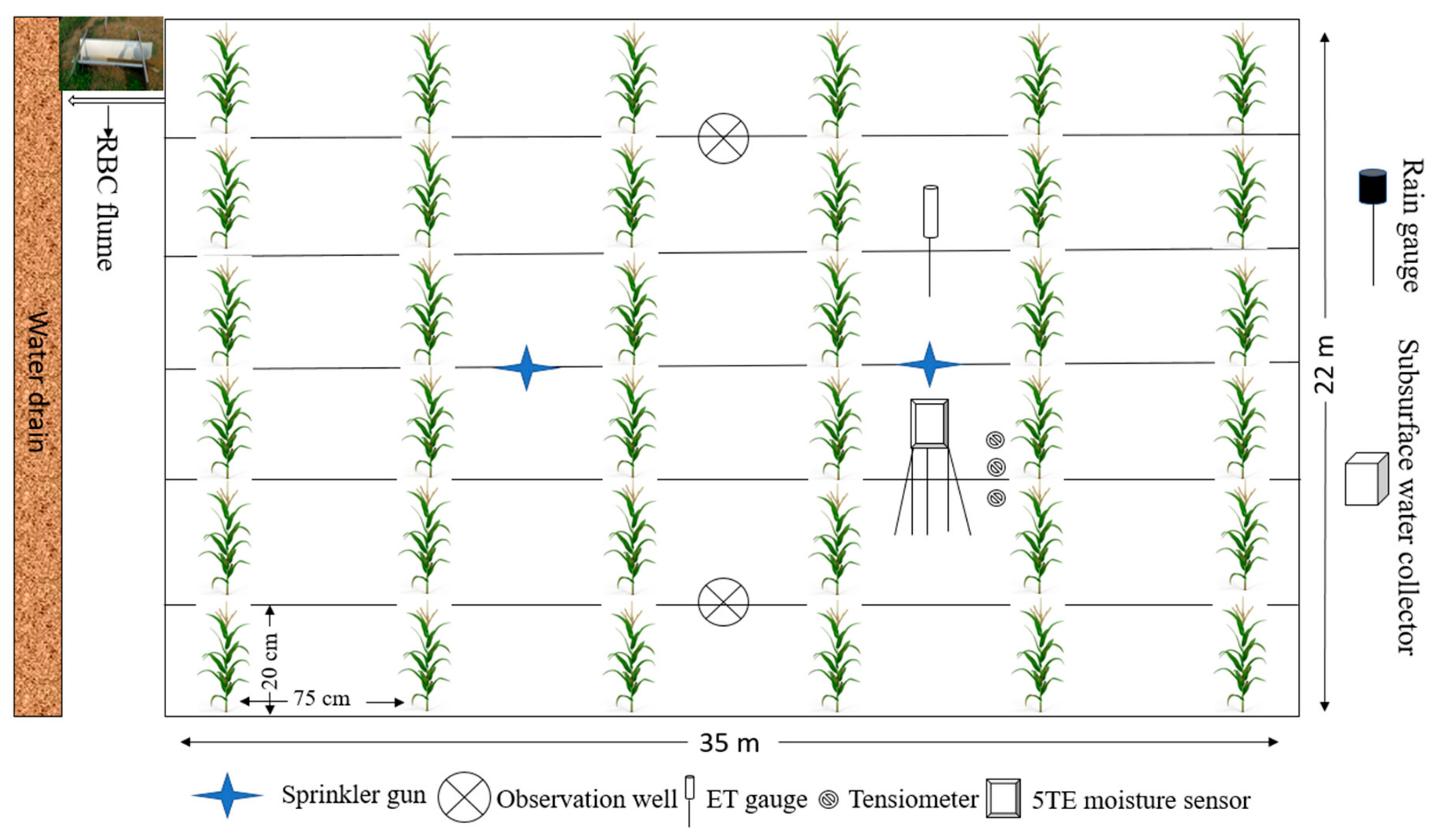
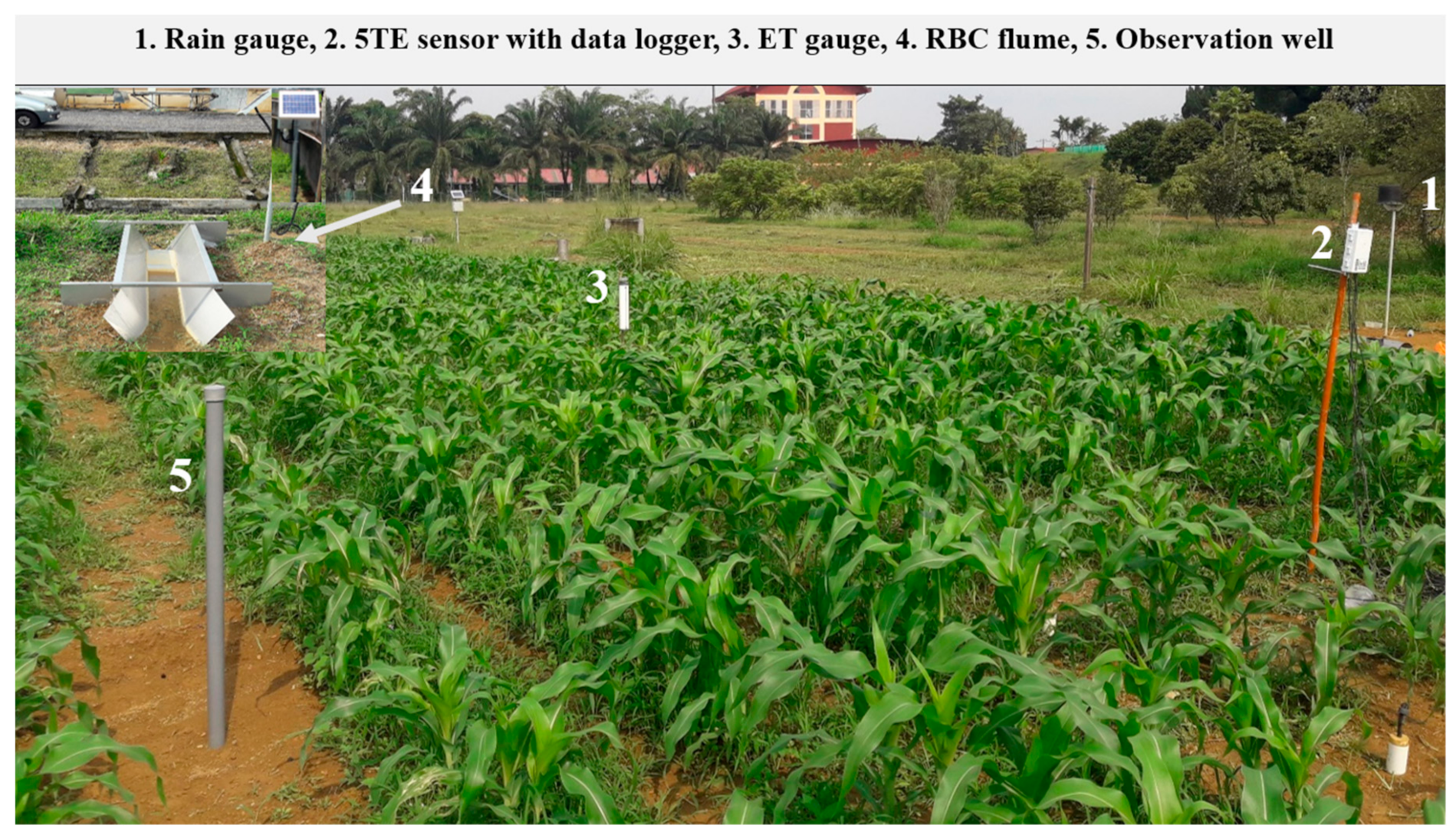
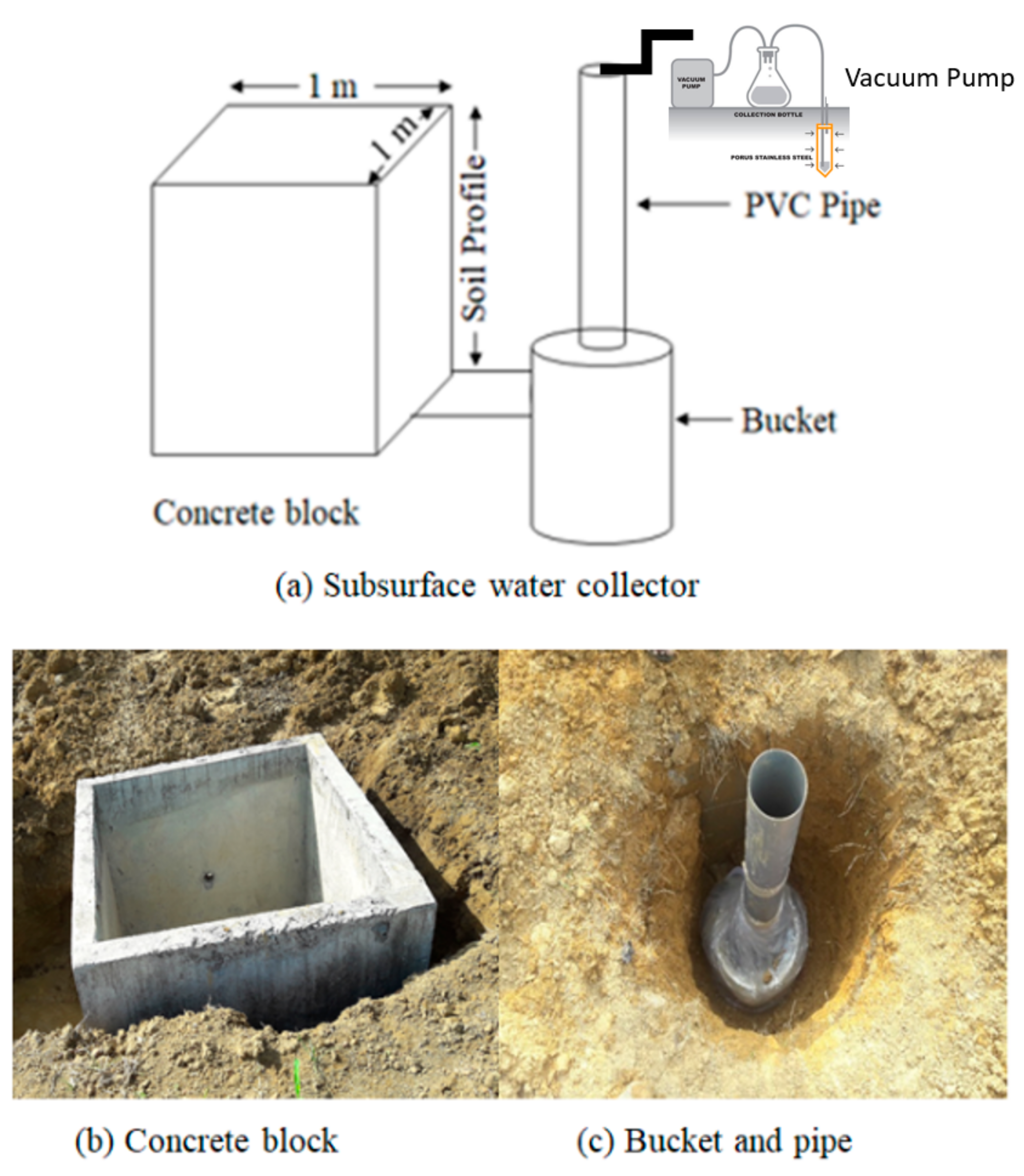
2.1. Field Experiments and Measurements
2.1.1. Site Description
2.1.2. Experimental Design and Measurements
2.1.3. Water Balance Components
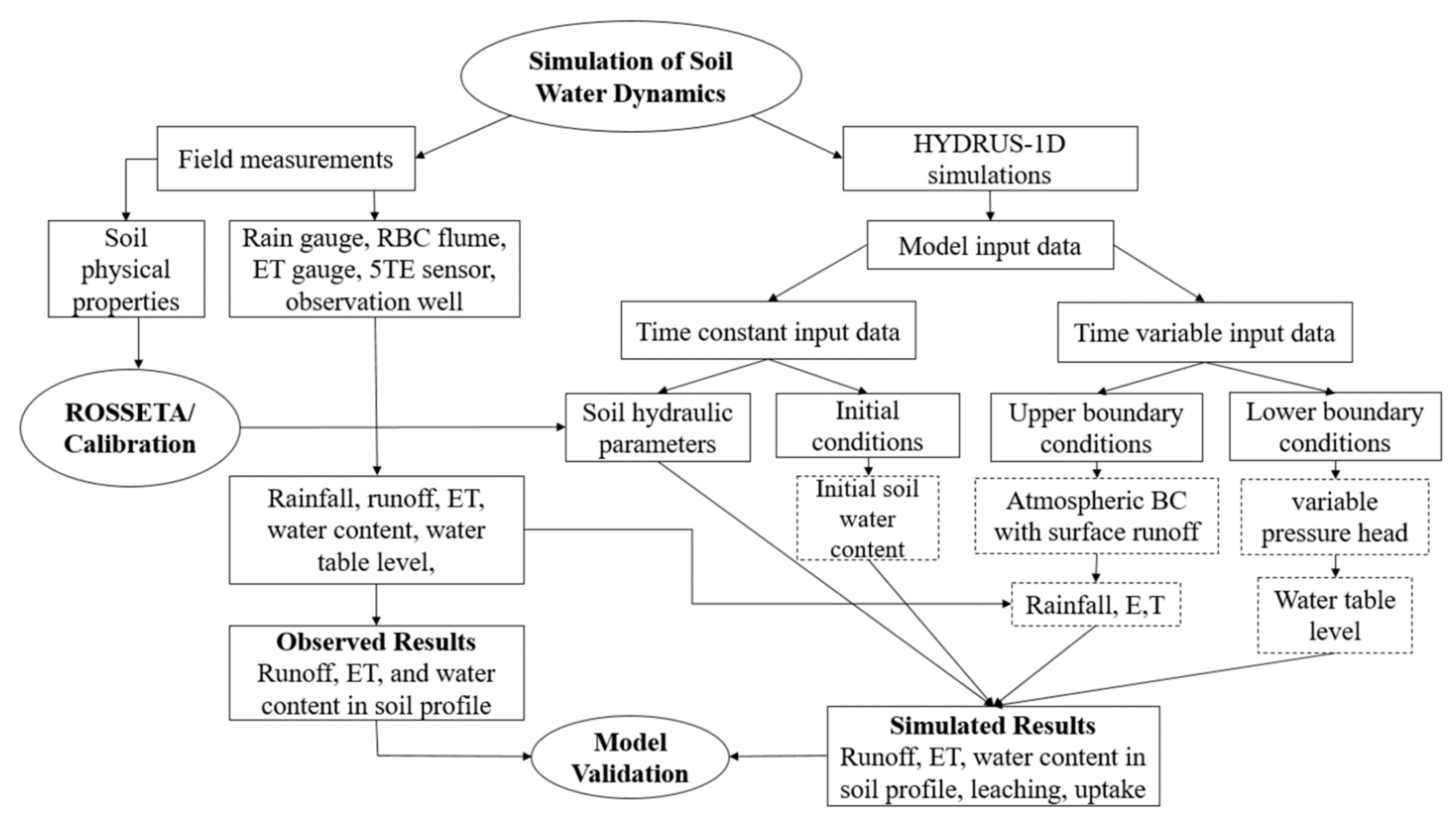
2.2. HYDRUS-ID Model
2.2.1. Model Description
2.2.2. HYDRUS-1D Input Parameters
Estimation of Soil Hydraulic Parameters
Estimation of Potential ET
Root Water Uptake
2.2.3. Initial and Boundary Conditions
2.3. Model Evaluation
2.4. Model Calibration and Validation
3. Results and Discussions
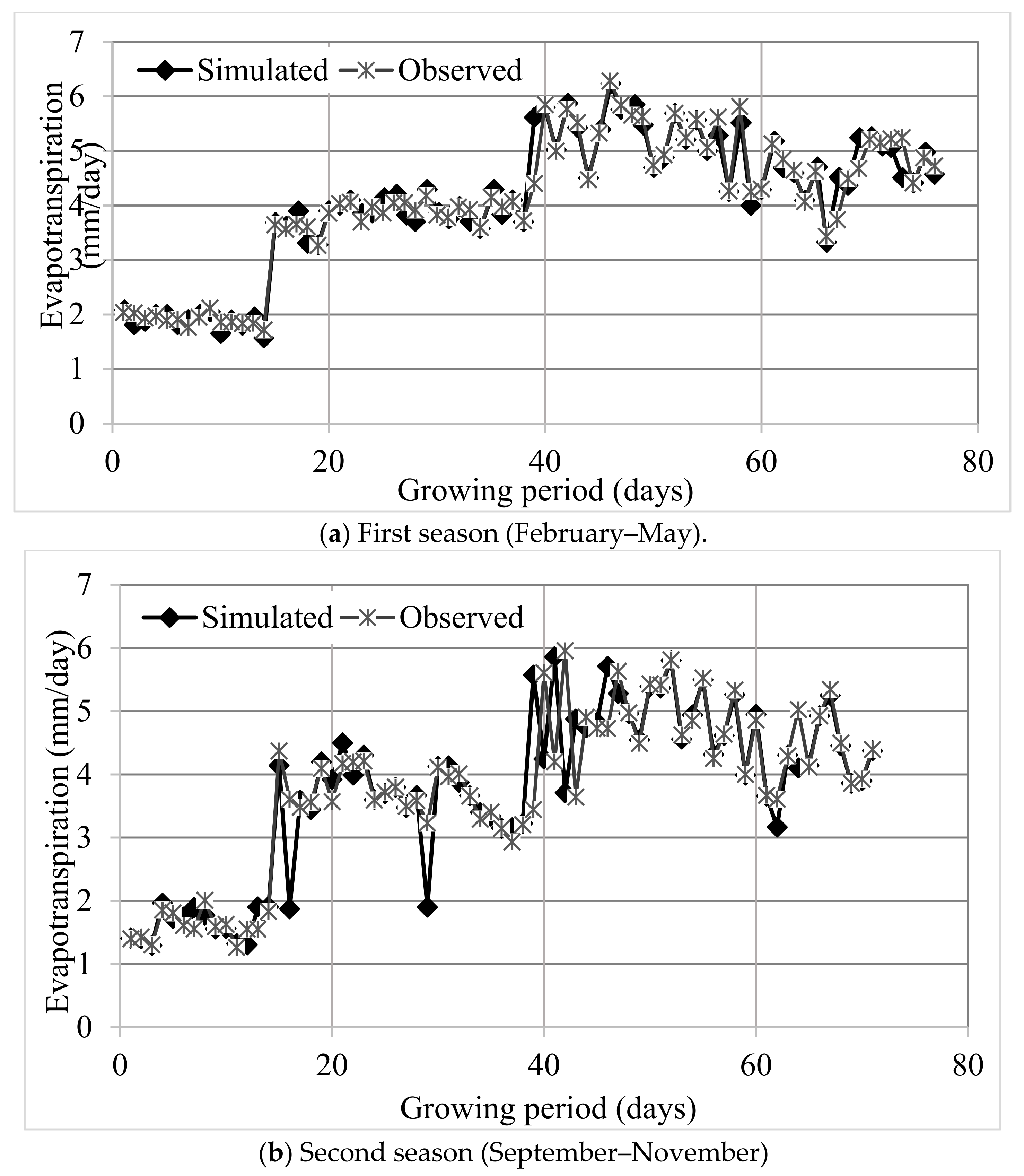
3.1. Evapotranspiration (ET)
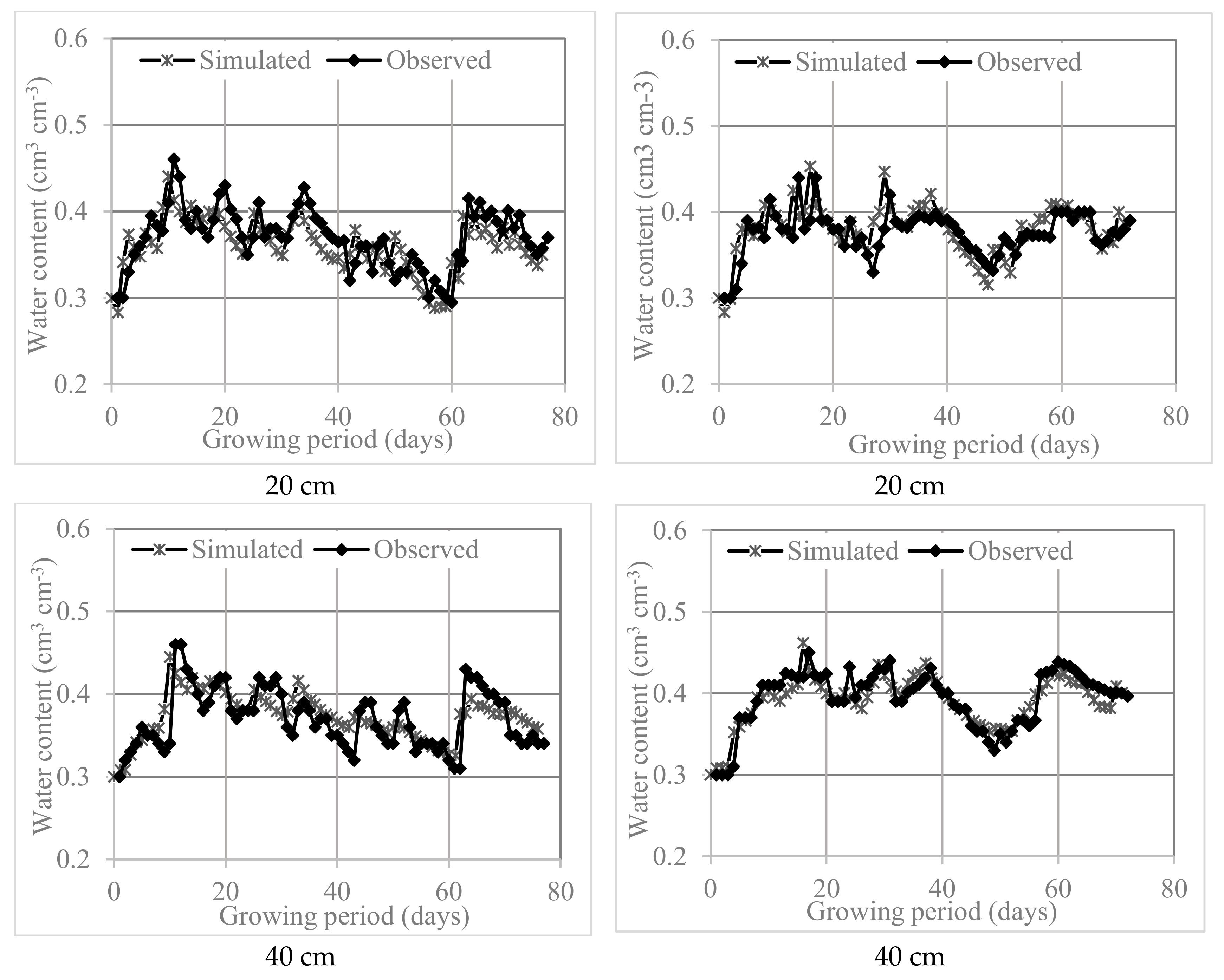
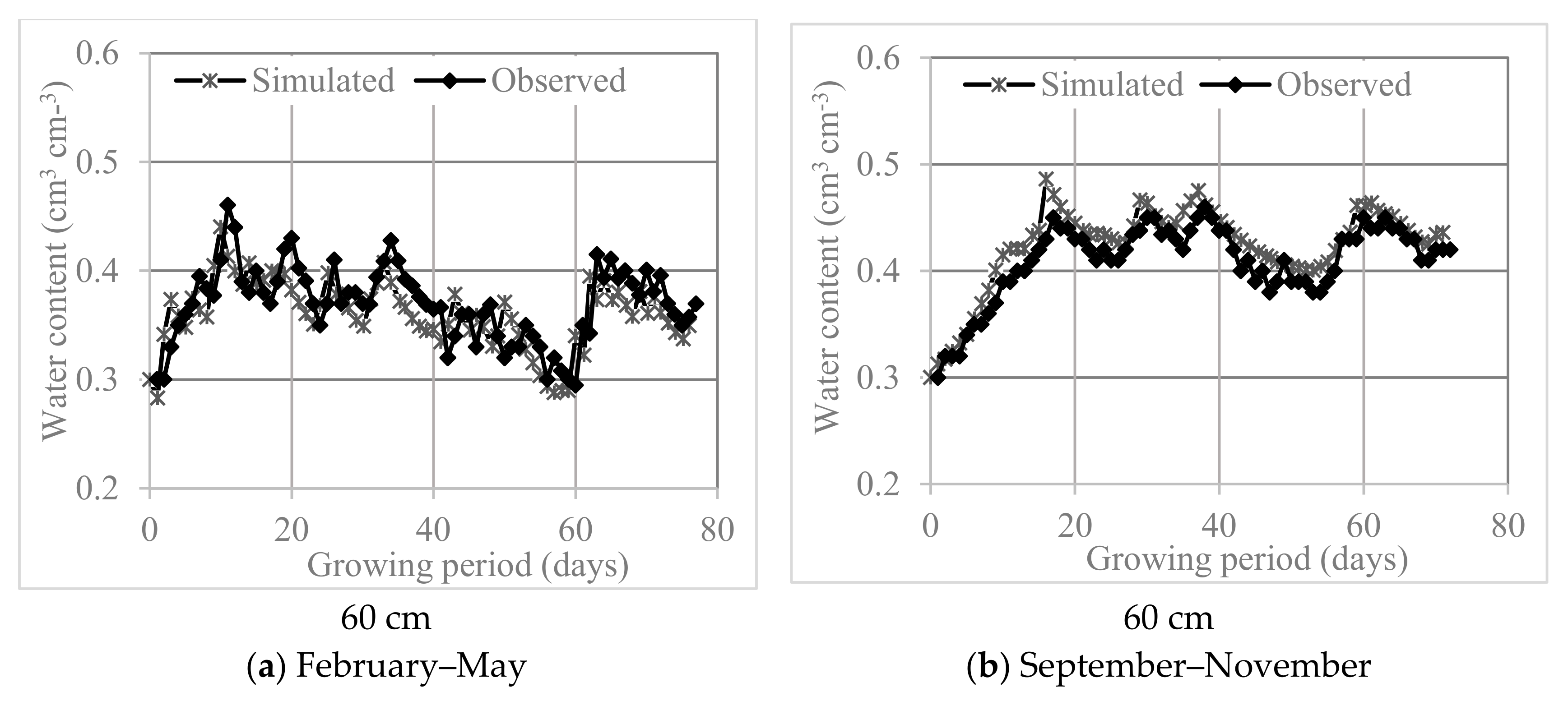
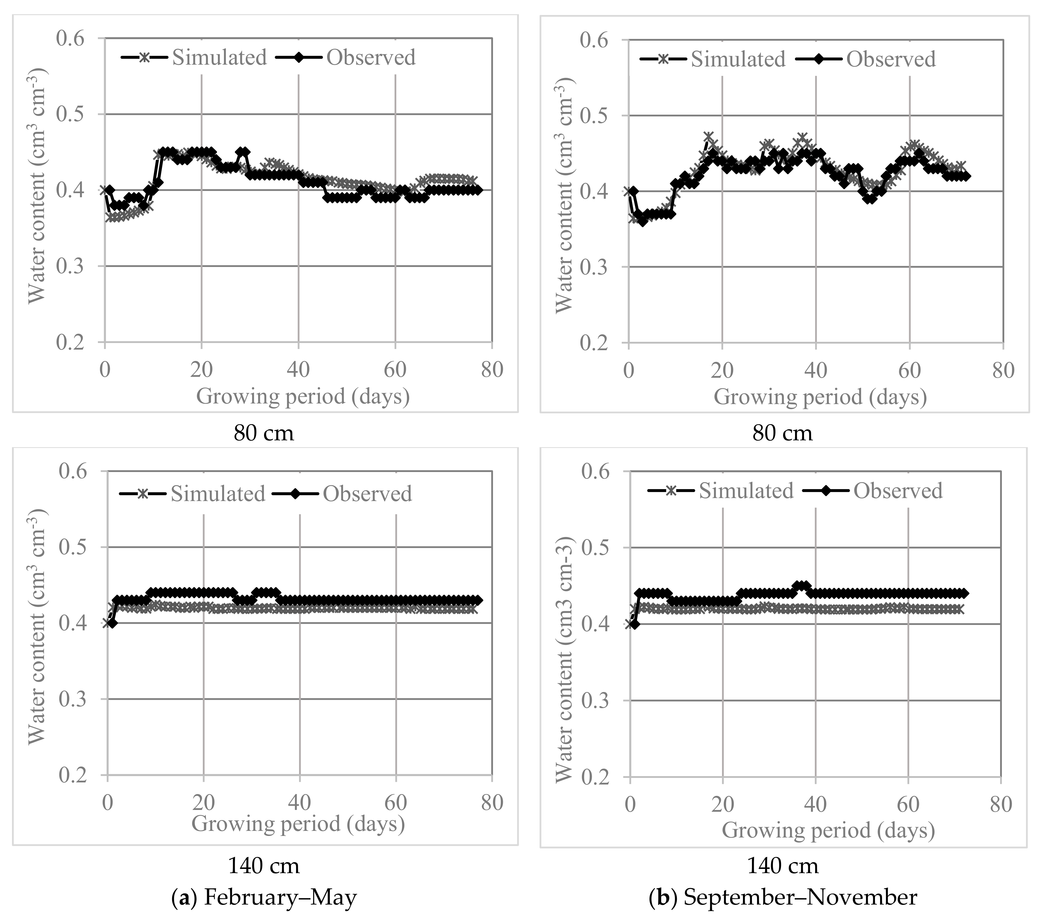
3.2. Water Contents
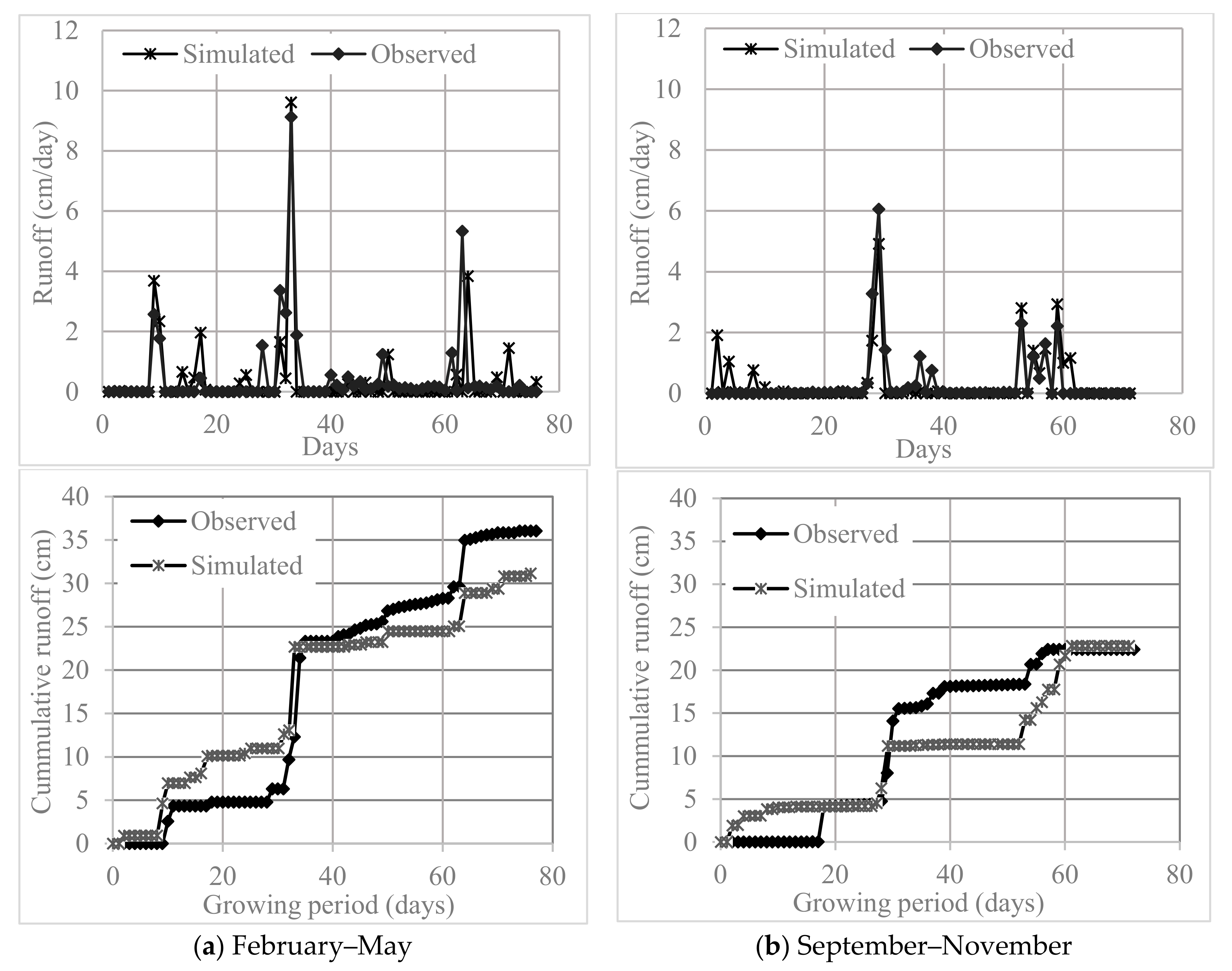
3.3. Surface Runoff
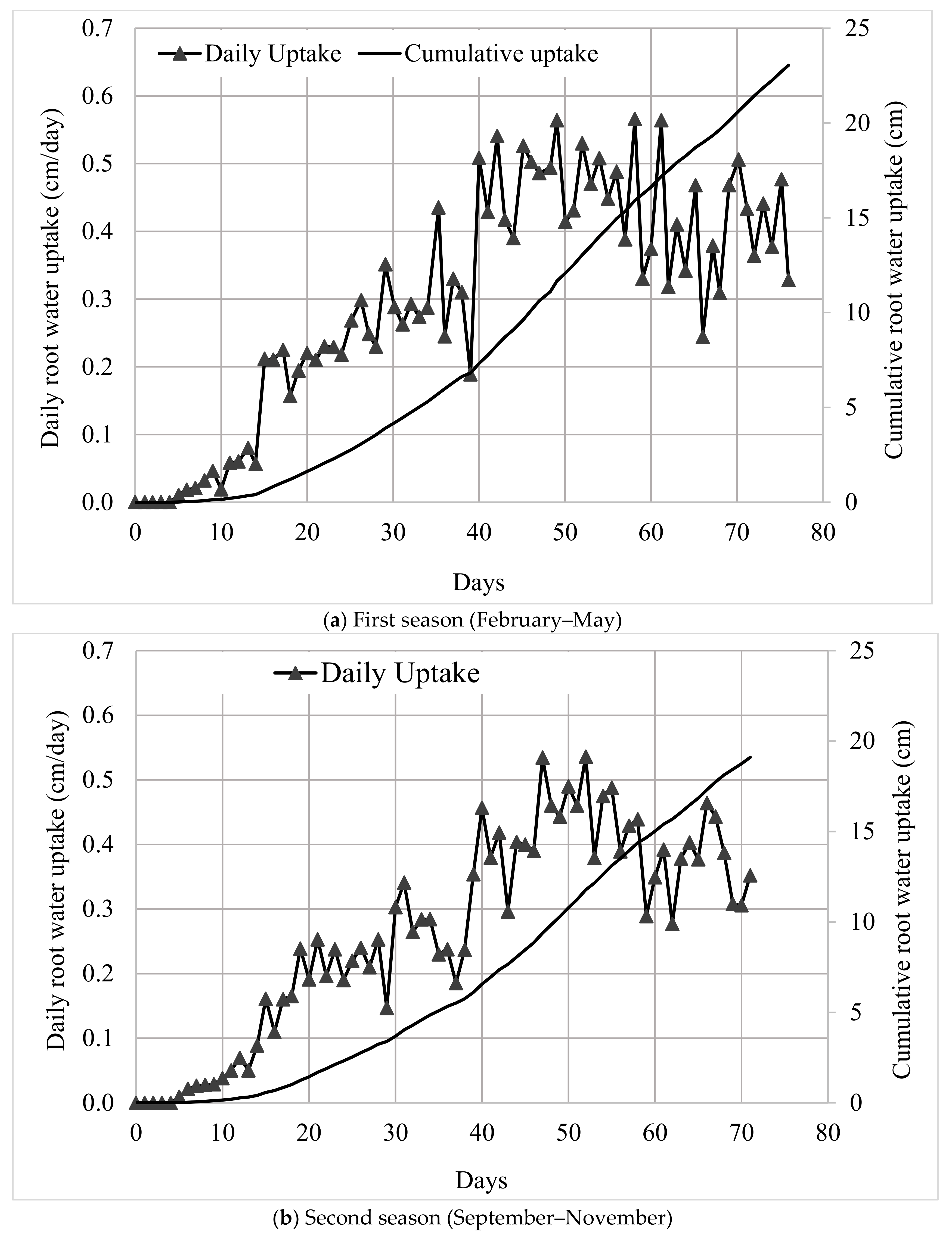
3.4. Root Water Uptake
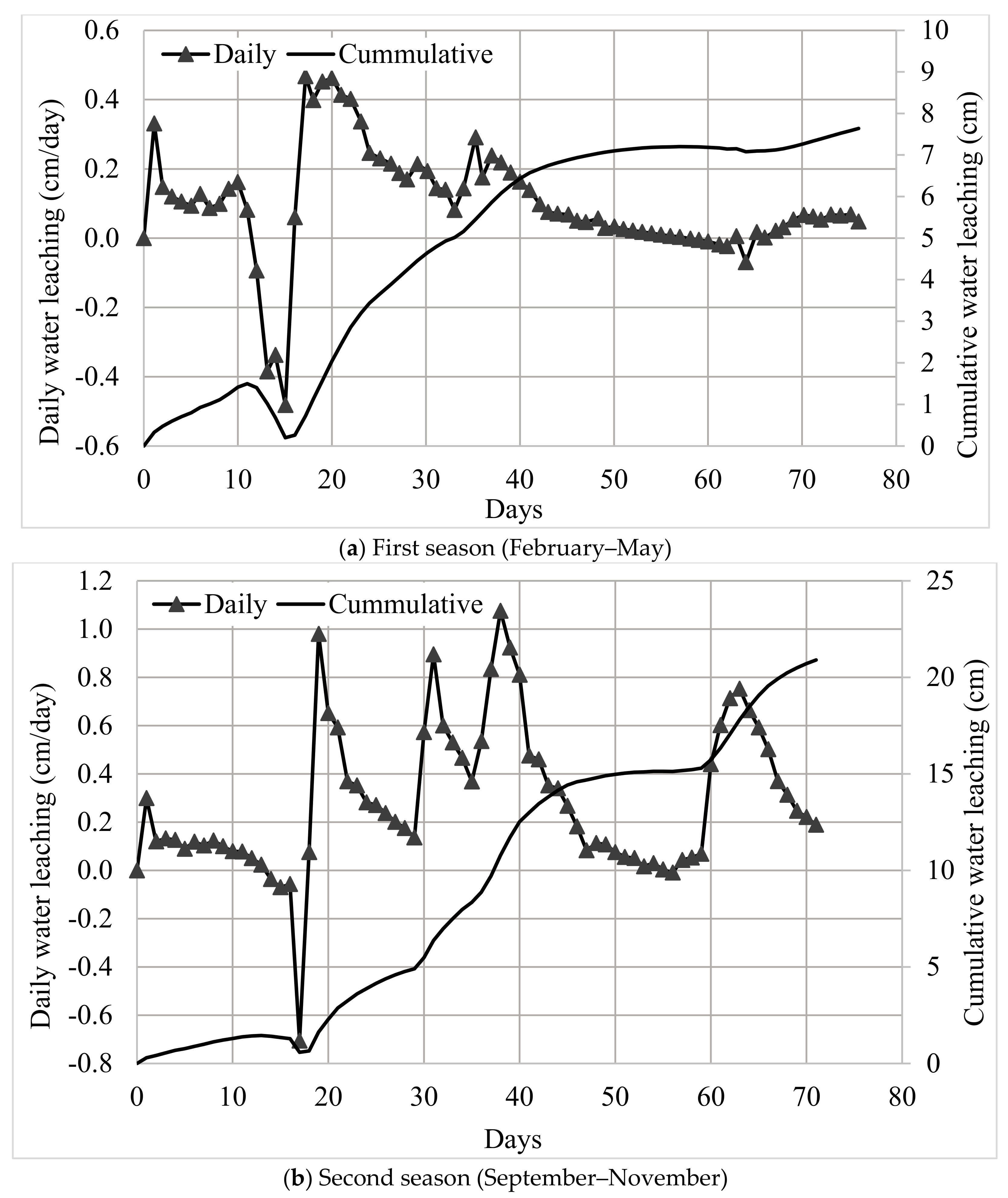
3.5. Water Leaching
3.6. Water Balance
4. Conclusions
Author Contributions
Funding
Acknowledgments
Conflicts of Interest
References
- USDA. United States Department of Agriculture, World Agricultural Production; Circular Series; USDA: Washington, DC, USA, 2018; Volume WAP 12–18.
- Wahab, A.G. GAIN REPORT: Grain and Feed Annual 2018; USDA Foreign Agricultural Service: Washington, DC, USA, 2018.
- DOA (Department of Agriculture). Vegetables and Cash Crops Statistic; Department of Agriculture: Putrajaya, Malaysia, 2017.
- Saeed, I.; Abassi, K.M.; Kazmi, M. Response of Maize (Zea mays, L.) to NP Fertilization under Agro-climatic Conditions of Rawalakot Azad Jammu and Kashmir. Park. J. Biol. Sci. 2001, 4, 949–952. [Google Scholar]
- Shamshuddin, J.; Sharifuddin, H.A.H.; Che Fauziah, I.; Edwards, D.G.; Bell, L.C. Temporal changes in chemical properties of acid soil profiles treated with magnesium limestone and gypsum. Pertanika J. Trop. Agric. Sci. 2010, 33, 277–295. [Google Scholar]
- Oad, F.C.; Buriro, U.A.; Agha, S.K. Effect of organic and inorganic fertilizer application on maize fodder production. Asian J. Plant. Sci. 2004, 3, 375–377. [Google Scholar]
- Shelia, V.; Šimunek, J.; Boote, K.; Hoogenbooom, G. Coupling DSSAT and HYDRUS-1D for simulations of soil water dynamics in the soil-plant-atmosphere system. J. Hydrol. Hydromech. 2018, 66, 232–245. [Google Scholar] [CrossRef]
- Igbadun, H.E. Estimation of Crop Water Use of Rain-Fed Maize and Groundnut Using Mini-Lysimeters. Pac. J. Sci. Technol. 2012, 13, 527–535. [Google Scholar]
- Wang, W.; Peng, S.; Yang, T.; Shao, Q.; Xu, J.; Xing, W. Spatial and temporal characteristics of reference evapotranspiration trends in the Haihe River basin, China. J. Hydrol. Eng. 2011, 16, 239–252. [Google Scholar] [CrossRef]
- Bruijnzeel, L.A. Predicting the hydrological impacts of land cover transformation in the humid tropics: The need for integrated research. In Amazonian Deforestation and Climate; John Wiley & Sons: New York, NY, USA, 1996; pp. 15–55. [Google Scholar]
- Watts, D.G.; Martin, D.L. Effects of water and nitrogen management on nitrate leaching loss from sands. Trans. ASAE 1981, 24, 911–916. [Google Scholar] [CrossRef]
- Šimůnek, J.; van Genuchten, M.T.; Šejna, M. Development and Applications of the HYDRUS and STANMOD Software Packages and Related Codes. Vadose Zone J. 2008, 7, 587–600. [Google Scholar] [CrossRef]
- Li, Y.; Šimůnek, J.; Zhang, Z.; Jing, L.; Ni, L. Evaluation of nitrogen balance in a direct-seeded-rice field experiment using Hydrus-1D. Agric. Water Manag. 2015, 148, 213–222. [Google Scholar] [CrossRef]
- Karandish, F.; Šimůnek, J. Two-dimensional modeling of nitrogen and water dynamics for various N-managed water-saving irrigation strategies using HYDRUS. Agric. Water Manag. 2017, 193, 174–190. [Google Scholar] [CrossRef]
- He, K.; Yang, Y.; Yang, Y.; Chen, S.; Hu, Q.; Liu, X.; Gao, F. HYDRUS simulation of sustainable brackish water irrigation in a winter wheat-summer maize rotation system in the North China Plain. Water 2017, 9, 536. [Google Scholar] [CrossRef]
- Ren, D.; Xu, X.; Hao, Y.; Huang, G. Modeling and assessing field irrigation water use in a canal system of Hetao, upper Yellow River basin: Application to maize, sunflower and watermelon. J. Hydrol. 2016, 532, 122–139. [Google Scholar] [CrossRef]
- Li, Y.; Šimůnek, J.; Jing, L.; Zhang, Z.; Ni, L. Evaluation of water movement and water losses in a direct-seeded-rice field experiment using Hydrus-1D. Agric. Water Manag. 2014, 142, 38–46. [Google Scholar] [CrossRef]
- Gabiri, G.; Burghof, S.; Diekkrüger, B.; Leemhuis, C.; Steinbach, S.; Näschen, K. Modeling spatial soilwater dynamics in a tropical floodplain, East Africa. Water 2018, 10, 191. [Google Scholar] [CrossRef]
- Ursulino, S.; Maria, S.; Lima, G.; Coutinho, A.P. Modelling soil water dynamics from soil hydraulic parameters estimated by an alternative method in an experimental basin located in the Brazilian Northeast region. Water 2019, 11, 1007. [Google Scholar] [CrossRef]
- Martello, M.; Dal Ferro, N.; Bortolini, L.; Morari, F. Effect of incident rainfall redistribution by maize canopy on soil moisture at the crop row scale. Water 2015, 7, 2254–2271. [Google Scholar] [CrossRef]
- Hou, L.; Zhou, Y.; Bao, H.; Wenninger, J. Simulation of maize (Zea mays L.) water use with the HYDRUS-1D model in the semi-arid Hailiutu River catchment, Northwest China. Hydrol. Sci. J. 2017, 62, 93–103. [Google Scholar]
- Negm, A.; Capodici, F.; Ciraolo, G.; Maltese, A.; Provenzano, G.; Rallo, G. Assessing the Performance of Thermal Inertia and Hydrus Models to Estimate Surface Soil Water Content. Appl. Sci. 2017, 7, 975. [Google Scholar] [CrossRef]
- Todorovic, M.; Lamaddalena, N.; Jovanovic, N.; Pereira, L. Agricultural water management: Priorities and challenges. Agric. Water Manag. 2014, 147, 1–3. [Google Scholar] [CrossRef]
- Van Genuchten, M.T. A closed-form equation for predicting the hydraulic conductivity of unsaturated soils. Soil Sci. Soc. Am. J. 1980, 44, 892–898. [Google Scholar] [CrossRef]
- Allen, R.G.; Luis, S.P.; Raes, D.; Smith, M. FAO Irrigation and Drainage Paper No. 56. Crop Evapotranspiration (guidelines for computing crop water requirements). Irrigation and Drainage 1998, 300, 300. [Google Scholar]
- Brouwer, C.; Heibloem, M. Irrigation Water Management: Irrigation Water Needs; Training Manual; Food and Agriculture Organization: Rome, Italy, 1986; Volume 3. [Google Scholar]
- Feddes, R.A. Simulation of Field Water Use and Crop Yield; Pudoc: Wageningen, The Netherlands, 1978. [Google Scholar]
- Nash, J.E.; Sutcliffe, J.V. River flow forecasting through conceptual models part I—A discussion of principles. J. Hydrol. 1970, 10, 282–290. [Google Scholar] [CrossRef]
- Schaap, M.G.; Leij, F.J.; Van Genuchten, M.T. Rosetta: A computer program for estimating soil hydraulic parameters with hierarchical pedotransfer functions. J. Hydrol. 2001, 251, 163–176. [Google Scholar] [CrossRef]
- González, M.G.; Ramos, T.B.; Carlesso, R.; Paredes, P.; Petry, M.T.; Martins, J.D.; Aires, N.P.; Pereira, L.S. Modelling soil water dynamics of full and deficit drip irrigated maize cultivated under a rain shelter. Biosyst. Eng. 2015, 132, 1–18. [Google Scholar] [CrossRef]
- Ramos, T.B.; Šimůnek, J.; Gonçalves, M.C.; Martins, J.C.; Prazeres, A.; Pereira, L.S. Two-dimensional modeling of water and nitrogen fate from sweet sorghum irrigated with fresh and blended saline waters. Agric. Water Manag. 2012, 111, 87–104. [Google Scholar] [CrossRef]
- Mo’allim, A.; Kamal, M.; Muhammed, H.; Yahaya, N.; Zawawe, M.; Man, H.; Wayayok, A. An assessment of the vertical movement of water in a flooded paddy rice field experiment using hydrus-1D. Water 2018, 10, 783. [Google Scholar] [CrossRef]
- Ramos, T.; Šimůnek, J.; Gonçalves, M.; Martins, J.; Prazeres, A.; Castanheira, N.; Pereira, L. Field evaluation of a multicomponent solute transport model in soils irrigated with saline waters. J. Hydrol. 2011, 407, 129–144. [Google Scholar] [CrossRef]
- Phogat, V.; Skewes, M.A.; Cox, J.W.; Alam, J.; Grigson, G.; Šimůnek, J. Evaluation of water movement and nitrate dynamics in a lysimeter planted with an orange tree. Agric. Water Manag. 2013, 127, 74–84. [Google Scholar] [CrossRef]
- López-Urrea, R.; Montoro, A.; Trout, T. Consumptive water use and crop coefficients of irrigated sunflower. Irrig. Sci. 2014, 32, 99–109. [Google Scholar] [CrossRef]


| Depth (cm) | Clay % | Silt % | Sand % | Textural Class | Bulk Density (g cm−3) | Conductivity Ks (cm d−1) |
|---|---|---|---|---|---|---|
| 0–20 | 65.36 | 09.79 | 24.84 | Clay | 1.36 | 12.86 |
| 20–40 | 53.28 | 15.24 | 31.45 | Clay | 1.39 | 12.43 |
| 40–60 | 58.66 | 13.12 | 28.23 | Clay | 1.31 | 12.78 |
| 60–80 | 70.20 | 20.22 | 09.58 | Clay | 1.22 | 18.11 |
| 80–140 | 71.74 | 18.03 | 10.23 | Clay | 1.24 | 17.56 |
| Depth (cm) | pH (Airdry) | EC umoh/cm | CEC cmol (+)/kg | Organic Matter %N | P mg/Kg | K mg/Kg |
|---|---|---|---|---|---|---|
| 0–20 | 6.87 | 62.80 | 5.88 | 0.14 | 55 | 74.1 |
| 20–40 | 5.95 | 64.90 | 5.68 | 0.12 | 26 | 74.1 |
| 40–60 | 6.20 | 45.75 | 6.49 | 0.12 | 39 | 19.5 |
| 60–80 | 5.80 | 41.47 | 7.47 | 0.11 | 30 | 42.9 |
| 80–140 | 5.98 | 85.78 | 7.13 | 0.09 | 22 | 19.5 |
| Depth (cm) | Soil Type | θs (cm3cm−3) | θr (cm3cm−3) | a (cm−1) | n | Ks (cm Day −1) | L |
|---|---|---|---|---|---|---|---|
| 0–20 | Clay | 0.0973 | 0.4750 | 0.0250 | 1.1625 | 12.86 | 0.5 |
| 20–40 | Clay | 0.0930 | 0.4561 | 0.0252 | 1.2019 | 12.43 | 0.5 |
| 40–60 | Clay | 0.0952 | 0.4661 | 0.0254 | 1.1828 | 12.78 | 0.5 |
| 60–80 | Clay | 0.1020 | 0.5084 | 0.0201 | 1.1903 | 18.11 | 0.5 |
| 80–140 | Clay | 0.1017 | 0.5066 | 0.0203 | 1.1825 | 17.56 | 0.5 |
| Season | Depth (cm) | R2 | EF | RMSE (cm3cm−3) |
|---|---|---|---|---|
| 1 | 0–20 | 0.72 | 0.73 | 0.017 |
| 20–40 | 0.72 | 0.63 | 0.021 | |
| 40–60 | 0.75 | 0.70 | 0.018 | |
| 60–80 | 0.67 | 0.65 | 0.012 | |
| 80–140 | 0.51 | −8.24 | 0.014 | |
| 2 | 0–20 | 0.84 | 0.70 | 0.013 |
| 20–40 | 0.85 | 0.82 | 0.014 | |
| 40–60 | 0.94 | 0.72 | 0.017 | |
| 60–80 | 0.82 | 0.69 | 0.013 | |
| 80–140 | 0.36 | −14.9 | 0.019 |
| Season | WI | ET | RO | L | SS | Ʃ | |
|---|---|---|---|---|---|---|---|
| First | Simulated | 75.8 | −30.88 | −31.10 | −07.64 | 3.70 | 2.48 |
| Observed | −30.84 | −36.00 | |||||
| Second | Simulated | 79.7 | −26.40 | −22.80 | −20.90 | 5.90 | 3.70 |
| Observed | −26.70 | −22.40 | |||||
© 2020 by the authors. Licensee MDPI, Basel, Switzerland. This article is an open access article distributed under the terms and conditions of the Creative Commons Attribution (CC BY) license (http://creativecommons.org/licenses/by/4.0/).
Share and Cite
Iqbal, M.; Kamal, M.R.; M., M.F.; Che Man, H.; Wayayok, A. HYDRUS-1D Simulation of Soil Water Dynamics for Sweet Corn under Tropical Rainfed Condition. Appl. Sci. 2020, 10, 1219. https://doi.org/10.3390/app10041219
Iqbal M, Kamal MR, M. MF, Che Man H, Wayayok A. HYDRUS-1D Simulation of Soil Water Dynamics for Sweet Corn under Tropical Rainfed Condition. Applied Sciences. 2020; 10(4):1219. https://doi.org/10.3390/app10041219
Chicago/Turabian StyleIqbal, Mazhar, Md Rowshon Kamal, Mohd Fazly M., Hasfalina Che Man, and Aimrun Wayayok. 2020. "HYDRUS-1D Simulation of Soil Water Dynamics for Sweet Corn under Tropical Rainfed Condition" Applied Sciences 10, no. 4: 1219. https://doi.org/10.3390/app10041219
APA StyleIqbal, M., Kamal, M. R., M., M. F., Che Man, H., & Wayayok, A. (2020). HYDRUS-1D Simulation of Soil Water Dynamics for Sweet Corn under Tropical Rainfed Condition. Applied Sciences, 10(4), 1219. https://doi.org/10.3390/app10041219