Article

Two-Stage Optimal Scheduling of Large-Scale Renewable Energy System Considering the Uncertainty of Generation and Load

1
Key Laboratory of Smart Grid of Ministry of Education, Tianjin University, Tianjin 300072, China
2
State Key Laboratory of Power Grid Safety and Energy Conservation (China Electric Power Research Institute), Beijing 100084, China
*
Author to whom correspondence should be addressed.
Appl. Sci. 2020, 10(3), 971; https://doi.org/10.3390/app10030971
Submission received: 30 December 2019 / Revised: 24 January 2020 / Accepted: 25 January 2020 / Published: 2 February 2020

Abstract

:
With the development of smart grid and low-carbon electricity, a high proportion of renewable energy is connected to the grid. In addition, the peak-valley difference of system load increases, which makes the traditional grid scheduling method no longer suitable. Therefore, this paper proposes a two-stage low-carbon economic scheduling model considering the characteristics of wind, light, thermal power units, and demand response at different time scales. This model not only concerns the deep peak state of thermal power units under the condition of large-scale renewable energy, but also sets the uncertain models of PDR (Price-based Demand Response) virtual units and IDR (Incentive Demand Response) virtual units. Taking the system operation cost and carbon treatment cost as the target, the improved bat algorithm and 2PM (Two-point Estimation Method) are used to solve the problem. The introduction of climbing costs and low load operating costs can more truly reflect the increased cost of thermal power units. Meanwhile, the source-load interaction can weigh renewable energy limited costs and the increased costs of balancing volatility. The proposed method can be applied to optimal dispatch and safe operation analysis of the power grid with a high proportion of renewable energy. Compared with traditional methods, the total scheduling cost of the system can be reduced, and the rights and obligations of contributors to system operation can be guaranteed to the greatest extent.

Graphical Abstract

1. Introduction

At present, a strong smart grid and ubiquitous power Internet of things are vigorously promoted in China. A high proportion of renewable energy is connected to the grid, and more comprehensive information about new energy, energy storage, and load is obtained by advanced technologies, such as artificial intelligence, sensors, and advanced communication technologies. Then, all data can be applied to optimal dispatching of power systems. Meanwhile, the global greenhouse effect has an increasing impact on the ecosystem, and CO2 emission reduction in the power industry plays a key role in reducing greenhouse gas emissions. The state grid of China is building “three types and two networks”, among which “three types”, namely hub type, platform type, and sharing type, are the characteristics of the enterprise. The “two networks”, namely the strong smart grid and the ubiquitous power Internet of things, are the material foundation. Under the strategy of “three types and two networks”, smart grid has a high penetration rate of new energy, so it is urgent to make full use of the generation-load-storage data to solve the low-carbon economic dispatch problem of wind power, PV (Photovoltaic) power generation, thermal power, energy storage, and other kinds of energy in multiple time scales.
On the one hand, this problem can be solved by the power generation side. The multi-energy complementary characteristics of fire, wind, light and energy storage power stations can be rationally used to mitigate the impact of new energy on the power grid. Replacing conventional power plants with renewable energy plants can significantly reduce the carbon emissions of the whole power system [1]. The charge-discharge characteristics of energy storage can solve the uncertainty related to wind and light power generation, and it also can alleviate line congestion to a certain extent [2]. The rapid development of large-scale renewable energy power stations has led to an explosive growth of dispatching data, and it is a challenge for power grid operation to establish scheduling plan by analyzing the characteristics and correlation of water, sunlight, wind and other new energy sources [3]. The BESS (Battery Energy Storage Station) has good peak regulation characteristics, which is used to reduce the influence of prediction error on wind power generation output in [4]. Meanwhile, an optimal scheduling model of thermal, wind, and storage system is proved to be superior in reducing the system operating cost. In [5], low load operation cost and slope climbing cost of thermal power units are concerned, and a day-ahead optimal scheduling model is established for wind power, photovoltaic, thermal power, pumped storage and energy storage power stations, and the dynamic inertia weight particle swarm optimization method is used to solve this problem. The uncertainty of generator failure, wind power, photovoltaic power generation, and load prediction is considered in [6], and a day-ahead dispatching optimization model is set with the system operating cost, reliability, and emission cost as the objective function. Considering wind power and PV volatility, a day-ahead, and real-time scheduling model is set for wind power, PV station with energy storage, and thermal power joint dispatching under the background of the power market in [7], and two-point estimation and genetic algorithm are used to solve them.
From the user side, the load curve can be optimized by actively guiding the user to participate in the demand response. The demand-side resources have a lot of influence on load peak reduction amount, among which electricity price-based demand response (PDR) accounts for 8%, and incentive-based demand response (IDR) accounts for the majority [8,9]. [10] points out that demand response and wind power generation have different variation characteristics, and the impact of wind power generation volatility on the power system can be alleviated by combining them. In [11], demand response and energy storage are introduced into the load side and the power generation side respectively, and the two-stage optimal scheduling model of wind and storage system is set based on the uncertainty of wind power output forecasts in the day-ahead and ultra-short period, and this model can be solved by chaos binary particle swarm optimization algorithm. Considering the deviation of wind power output prediction and user response in multiple time scales, an interactive decision-making model between the day-ahead and the intraday stage is set for wind power, demand response, and emergency peak regulation resources in [12]. Based on the uncertain model of market price, load, wind speed, temperature, and radiation, the compressed air storage and PDR are introduced to solve the random self-regulation problem of renewable energy in [13], and the proposed method can reduce the system operating cost by simulation. Considering the uncertainty of high load and wind power generation, a scheduling model is established to minimize the total cost of system operating and sewage discharge in [14]. Similarly, a joint optimal schedule method is proposed for wind-solar-water complementary power generation system and high energy consumption data center in [15]. In [16], considering wind, thermal, storage, and demand response on both sides of generation-load, a two-stage optimal scheduling model is established based on the interval method to simulate wind power scenarios.
The above literature mainly focuses on the day-ahead dispatching of various renewable energy, and the volatility of large-scale new energy generation cannot be ignored. On the user side, the demand response scheduling strategy with multiple time scales attracts the most scholars, and the joint scheduling with multiple energy sources attracts less attention. Meanwhile, with the gradual deepening of building a strong smart grid, the permeability of renewable energy continues to increase, and its intermittently and volatility bring great difficulties to the peak regulation of the grid. Thermal power units will often be in the state of severe peak load regulation and frequent climbing [17], and the impact on the operating cost of the system cannot be ignored.
The scheduling mode combining day-ahead dispatching and real-time automatic generation control is widely used in China, but its scheduling stage span is too large. With the grid connection of large-scale new energy generation, the capacity requirements of real-time AGC (Automatic Generation Control) units are becoming higher and higher [18,19]. As the uncertainty of source-charge decreases with time, intraday rolling scheduling can be added into the scheduling mode to complete load distribution in a shorter time scale based on the day-ahead scheduling plan and update the day-ahead generation plan in a rolling manner.
Based on this, this paper comprehensively considers the characteristics of wind, solar, thermal units and demand response in different time scales, and proposes a day-ahead and intraday scheduling model to solve the low-carbon economic dispatch problem of multiple energy. In this model, the uncertainty model of day-ahead price demand response virtual units and intraday IDR virtual units are established, and the operation cost and slope climbing cost of thermal power units in deep peak regulation are concerned. Considering the wind and light output fluctuation on the power generation side and the uncertainty of demand response on the load side, a low-carbon economy optimization scheduling model is set for the multi-energy system, which is calculated by the improved bat algorithm and two-point estimation method. The effectiveness and rationality of this two-stage optimal scheduling method are analyzed by the example results.
The main contributions of this paper are as follows:
(1) Under the background of “three types two nets” strategy and low-carbon electricity, large-scale renewable energy is integrated into the power grid and the peak-valley difference of system load increases. In a multi-energy scheduling system of wind-solar-thermal plants and BESS, the unit output adjustment can be reduced by making full use of many complementary energy features on multiple time scale, and it is beneficial to realize the optimal low-carbon economic dispatch.
(2) Considering the source-load interaction in multiple time scales, the user-side demand response is divided into the day-ahead price-type response virtual unit and intraday incentive response virtual unit. In addition, they are expressed with triangular membership functions and uniform distribution. The fluctuation of wind and solar on the power generation side is described by a probability density function. Then the influence of generation-load prediction error on a multi-energy collaborative scheduling system can be analyzed, and the optimal scheduling plan can be determined.
(3) Due to the high proportion of renewable energy integrated into the grid, the volatility and intermittency of new energy sources increase the peak load regulation pressure of the power system. To keep the system running safely and stably, thermal power units frequently climb hills and are often in deep peak regulation state, which will increase coal consumption. These effects on the optimal scheduling model cannot be ignored.
(4) The genetic algorithm is introduced into bat algorithm to make bats possess the genetic characteristics of the genetic algorithm so that the solution accuracy and global search ability of the algorithm are improved, and this new bat algorithm is applied to solve the optimal scheduling plan in the wind-PV-thermal-storage joint scheduling system.
The remaining of this paper is organized as follows: Section 2 describes the scheduling mode of the wind-PV-thermal-storage system when demand response is considered. Section 3 describes the uncertainty model of generation and load. Section 4 describes a two-stage optimal scheduling model for the wind-PV-thermal-storage system and its solutions. Section 5 describes a specific example study and the analysis of the results. Conclusions are drawn in Section 6.

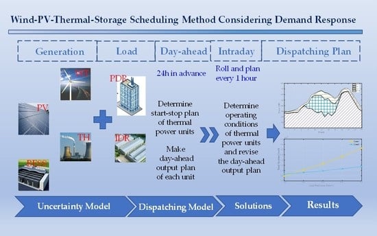
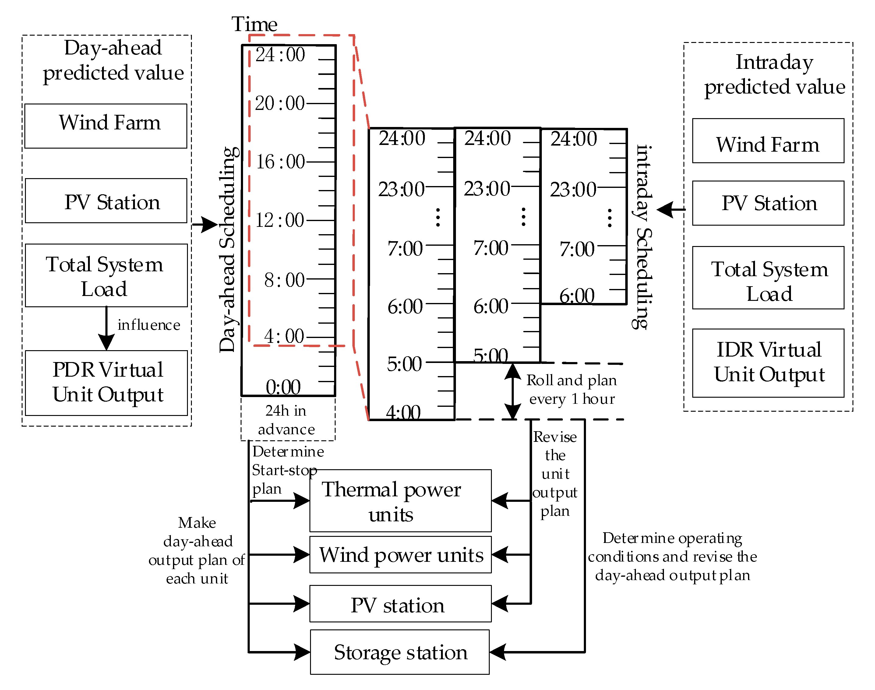
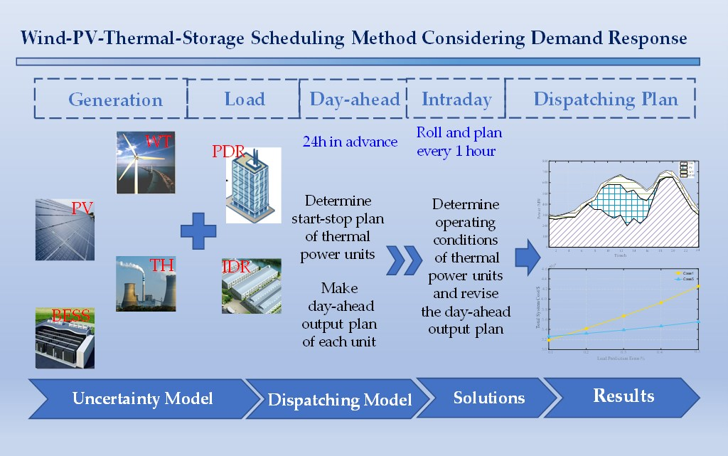
2. Wind-PV-Thermal-Storage Scheduling Mode Considering Demand Response

Further development of the energy revolution and the digital revolution has let the smart grid and the Internet of things continue to merge and develop. Among them, the smart grid is characterized by informatization, automation and interaction, and the Internet of things can realize intelligent identification, tracking, monitoring, and management of goods based on the Internet and traditional telecommunication network. These technologies make demand-side resources can be flexibly scheduled, which is conducive to the interaction between users and the power grid. In addition, it is helpful to achieve peak load cutting and valley filling and improve the absorption rate of renewable energy. The wind-PV-thermal-storage scheduling model considering demand response consists of two stages, as shown in Figure 1.
The day-ahead scheduling is implemented one day in advance, and the total dispatching cycle is 24 h, unit time of 1 h. The power grid department informs the price demand response users in advance and predicts the system load of the next day. In addition, the dispatching center receives the predicted output values of each wind farm and photovoltaic power station on the next day and arranges the output of each thermal power unit, wind farm, photovoltaic station, and storage station in the next day. Considering that the thermal power unit start–stop is time consuming, high cost, and time price cannot be changed after the release, the thermal power unit start–stop combination and price demand response are determined in the day-ahead stage, which cannot be changed in the intraday stage.
The intraday scheduling is carried out 15 min in advance, and the whole dispatching cycle is 1 h. The output of units, energy storage power station, and IDR at each time period are revised in a rolling manner. The power grid department informs intraday demand response users in advance and gets the ultra-short predicted values of the wind farm and photovoltaic power station. In addition, the intraday system load considering the day-ahead demand response is calculated at this stage to correct the output of the started thermal power unit and determine the intraday demand response and energy storage power station output.

3. Generation-Load Uncertainty Model

Due to the access of wind power, photovoltaic power station, load integrator, and energy storage power station, the stability of the power system is facing challenges. To solve the optimal scheduling problem of the power system containing renewable energy, it is necessary to describe the uncertain model of light intensity, wind speed, load, and demand response.

3.1. Uncertain Models of Renewable Energy Output

Currently, good commercial renewable power generation includes controllable generation forms (such as hydroelectricity) and intermittent uncontrollable renewable energy (such as wind and solar). This part only analyzes the uncontrollable power generation model adopted in the dispatching decision-making process.

3.1.1. PV Output Uncertainty Model

The output of photovoltaic power station depends on the solar illumination intensity, and the functional between the output of a PV power station P PV and the illumination intensity R is as follows:
P PV ( R ) = { P PV ,   r ( R 2 R std R c ) 0 < R < R c P PV ,   r ( R R std ) R < R c
where P PV ,   r is the rated output power of photovoltaic power station, R std is the light intensity in a standard environment, 1000 W/m2, and R c is the light intensity of a certain position, 150 W/m2.
For a certain location, the light intensity per hour obeys a dual-mode distribution, i.e., the combination of two single-mode distribution functions such as Weibull, Beta, and other probability density functions. PV output is greatly affected by weather factors, so it is meaningful to discuss the different PV output under different environmental conditions, which is not the focus of this paper. Therefore, this paper does not consider the influence of clearness indexes on PV output.

3.1.2. Wind Power Output Uncertainty Model

Wind turbine output is related to wind speed, and its probability distribution function is recorded and statistically analyzed. It can be found that wind speed follows the Weibull probability density function, and the corresponding wind turbine power distribution can be expressed.
Compared with wind speed, wind power output is random. For a given wind speed input, the output power of the wind turbine is:
P W ( v ) = { 0 v < v in ,   v > v out P W ,   r ( v v in v r v in ) v in v v r P W , r v r < v < v out
where P W , r is the rated output power of the wind turbine, v in , v out , and v r are cut-in wind speed, cut-off wind speed, and rated wind speed, respectively.

3.2. Load Uncertainty Model Considering Demand-Side Management

At any time, the system load demand at the next time is uncertain, and the load demand uncertainty can be modeled by normal distribution and uniform distribution probability density function. In this paper, the probability density function of a normal distribution is used to model the system load before participating in the demand response.
P L , t , act = P L , t P DR , t
where P L , act , t is the actual power of the system load after participating in the demand response at time t, P L , t is the load power of the system at this moment, P DR , t is the demand response power of the user at time t, which includes price demand response and IDR.

3.2.1. Uncertainty Model of Day-Ahead Price Demand Response Virtual Unit

The electricity consumption behavior of users in the electricity price demand response is fixed, and the response time is long, but the adjustable range is limited. In the day-ahead dispatching stage, the electricity price mechanism is used to guide users to choose more economical electricity consumption mode, so that load can be flexibly adjusted. Under the background of the energy Internet of things and the strong smart grid system, the number of users participating in demand response increases. Therefore, it is necessary that electricity price demand response in a specific area should be assembled into a virtual unit for scheduling, named a price demand response virtual unit. The decision variable of this virtual unit is the electricity price, i.e., the change of the price mechanism affects the output of the virtual unit.
The demand response based on the price elasticity coefficient is studied from the economic point of view. When the electricity price is high, less electricity is used. On the contrary, more electricity is used. The power sector adjusts the user’s electricity consumption through the electricity price. The influence of the price change rate on the load change rate is represented by the self-elastic coefficient, which is defined as follows:
ϕ Δ L , t = e t t × ϕ Δ ρ , t
where ϕ Δ L , t is the load response rate of price response virtual unit at time t, ϕ Δ ρ , t is the price change rate at time t, and e t t is the self-elasticity coefficient at time t.
Users participate in the demand response according to the voluntary principle. The actual response quantity of load is random and cannot be completely determined. In this paper, the triangular membership function is used to describe the uncertainty of the PDR load response rate:
ϕ ˜ Δ L , t = ( ϕ Δ L 1 , t , ϕ Δ L 2 , t , ϕ Δ L 3 , t ) { ϕ Δ L 2 , t = e t t ϕ Δ ρ , t ϕ Δ L 1 , t = ϕ Δ L 2 , t Δ δ t ϕ Δ L 3 , t = ϕ Δ L 2 , t + Δ δ t
where ϕ ˜ Δ L , t is the fuzzy expression of load response rate ϕ Δ L , t in time period t. ϕ Δ L 1 , t , ϕ Δ L 2 , t and ϕ Δ L 3 , t are membership parameters. e t t is the self-elastic coefficient of the price elasticity matrix in time period t. Δ δ t 0 , is the maximum error value of load response rate prediction at time t, which is related to the price change rate and the detailed calculation process is shown in [20].
The triangular numbers in the fuzzy expression of load demand response rate are converted into a certain variable, then the expected value of them can represent the users’ actual response quantity due to price changes [21], as follows:
P PDR , t , act = 1 4 P PDR , t ( ϕ Δ L 2 , t + 2 ϕ Δ L 1 , t + ϕ Δ L 3 , t )
where P PDR , t , act is the PDR users’ actual response power in day-ahead stage at time t, P PDR , t is the system load when the users do not participate in the price demand response at time t.

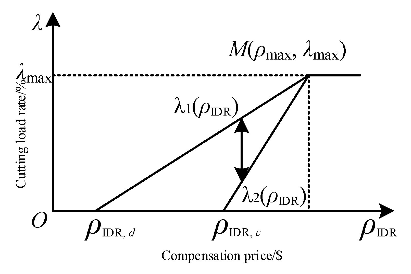
3.2.2. Uncertainty Model of Intraday IDR Virtual Unit

The users of IDR have a short response time and a large elastic margin. The users participating in IDR in a certain area can be gathered into a virtual unit, and the power company adopts the incentive mode of ladder compensation price to dispatch in the intraday stage, so as to realize the rapid increase or decrease of load in the power system operation. According to the IDR curve shown in Figure 2, it can be known that users’ cutting load rate λ fluctuates within a range [ λ 2 ( ρ IDR ) , λ 1 ( ρ IDR ) ] at a certain compensation price ρ IDR . The uncertainty of users’ response at a certain incentive level can be simplified into uniform distribution:
λ ( ρ IDR ) = 1 λ 1 ( ρ IDR ) λ 2 ( ρ IDR )
where λ ( ρ IDR ) is the cutting load rate of the incentive response virtual unit under the incentive price ρ IDR λ 1 ( ρ IDR ) and λ 2 ( ρ IDR ) are the upper and lower limits of the cutting load rate respectively, and the calculation formula is referred to in the [22].
The actual response quantity P IDR ,   t , act of IDR users in the intraday stage is:
P IDR , t , act = λ IDR , t P IDR , t
where λ IDR , t is the cutting load rate of IDR virtual unit at time t, and P IDR , t is the power when users’ do not participate in the incentive demand response at time t.

4. A Two-Stage Optimal Scheduling Model for Wind-PV-Thermal-Storage System

In this paper, an optimal scheduling method is proposed for hybrid power generation systems to reduce the impact of renewable energy generation uncertainty on power system operation, and this system includes thermal power, wind power, PV power generation, and battery energy storage stations. In fact, the output of wind power and photovoltaic power generation is mainly predicted by the weather forecast and these are involved in dispatching. Due to the fluctuation of wind speed and Intermittence of light intensity, this paper simulates the output of wind power and photovoltaic power based on the probability distribution function.

4.1. Day-Ahead Optimal Scheduling Model

4.1.1. Low-Carbon Economy Scheduling Objective Function

To realize low-carbon power, carbon emission cost is introduced into economic dispatch objective function of the power system:
min F = F 1 + t = 1 T C tax ( E C , t E D , t )
where F 1 is the cost function of system operation. $. C tax is the unit carbon treatment cost in the market, $/ton. E C , t is the thermal power unit carbon emissions, ton. E D , t is the carbon allocation amount of the generator unit in time period t, ton. When the unit’s carbon emission is within the range of carbon allocation, the carbon treatment cost is 0. T is the number of segments in the scheduling cycle and T = 24 in day-ahead scheduling.
Wind power and photovoltaic power generation are renewable energy sources, so there is no carbon emission in the power generation process. In addition, their carbon emission is not considered in the solving process. The carbon emission in the power system comes from the coal consumption of thermal power units. The carbon emission allocation quota of generators in the time period t is as follows:
E D , t = i = 1 N F η D P F , i , t
where N F is the number of thermal units, and η D is the carbon emission allocation of generator’s unit active power output.
The actual carbon emission of thermal power units during the period t [23] is:
E C , t = i = 1 N F ( α i P F , i , t 2 + β i P F , i , t + δ i )
where α i , β i , δ i are emission factors of thermal power units, respectively.

4.1.2. Economy Scheduling Objective Function

The optimal scheduling strategy is the joint operation of thermal power plants and renewable energy power plants. The objective function is to minimize the operating cost of the system:
F 1 = t = 1 T ( f G , t + f GO , t + f E , t + f DR , t )
where f G , t , f GO , t , f E , t , f DR , t are the generation cost and dispatching cost of multiple power sources, the charging and discharging cost of energy storage stations, and the dispatching cost of demand response at time t.
The first item is the power operation cost, including the operation and dispatching cost of thermal units, and the operation and maintenance cost of renewable energy generators.
f G , t = f F , t + f W , t + f PV , t
where f F , t , f W , t , f PV , t are respectively thermal power unit operating cost, wind power, and photovoltaic power generation operation and maintenance cost in each period.
• The Operating Cost of Thermal Power Units
Due to the large-scale renewable energy with volatility into the grid, the climbing number and start times of traditional thermal power units increase. Therefore, the cost of deep peak adjustment cannot be ignored.
According to the characteristics of the steam turbine, the heat rate will be higher, and the unit life loss will be bigger when the load of the steam turbine is lower. The cost of deep peak adjustment [24] includes coal consumption cost of unit operation and unit loss cost during severe peak load regulation. Thermal power units can be divided into normal operation state and deep peak regulation state during operation. The thermal power unit operation cost is:
f F , t = i = 1 N F [ u F , i , t   ( a i P F , i , t 2 + b i P F , i , t + c i + w cos t , i ) ]
where u F , i , t is the start–stop variable of the thermal power unit and the value is 1 or 0, P F , i , t is the output of the i-th thermal unit, a i , b i , c i are the fuel cost coefficients of the i-th thermal unit in normal operation. When the thermal unit is severe peak load regulation state, the thermal stress of the rotor is too large to cause unit loss cost and w cost , i is the additional operating cost of deep peak adjustment, and the calculation formula is:
w cost , i = { 0 P F , i α P F , i , max χ C unit 2 N f ( P F , i ) other
where α represents the boundary of the low-load state, and usually is 0.6, χ is the actual operating loss coefficient of the thermal power unit, N f ( P F , t ) is the cycle times of rotor cracking, which is determined by the low cycle fatigue characteristics of rotor material, and C unit is unit purchase cost.
• Operation and Maintenance Cost of Renewable Energy
Wind and photovoltaic power generation do not consume fuel, but the randomness and volatility of wind and light will affect the normal operation of the unit and generate a certain operation and maintenance cost, which can be approximately expressed as the linear function of unit generating power [25].
f W , t = j = 1 N W P W ,   j , t ρ W , j
f PV , t = k = 1 N PV P PV , k , t ρ PV , k
where N W N PV are the number of wind power units and PV power units, ρ W , j , ρ PV , k are the operation and maintenance cost coefficient of the wind farm and PV station, P W ,   j , t , P PV , k , t are the restricted active power output of wind farm and photovoltaic at time t respectively.
The second is the power dispatching cost, including the start-up and climbing cost of thermal power units and the restricted generating cost of renewable energy units.
f GO , t = C F 1 , i + C F 2 , i + C WL , i + C PVL , i
• The Start–Stop Cost and Slope Climbing Cost of Thermal Power Plants
When large-scale renewable energy is connected to the grid, its intermittency and volatility will lead to frequent start–stop and slope climbing of thermal power units, which will increase operating costs. The start–stop and climbing cost function is as follows:
C F 1 , i = u F , i , t ( 1 u F , i , t 1 ) S F , i , t
C F 2 , i , t = γ F | d P F , i , t d t |
where u F , i , t is the number of starting thermal power units in time period t, S F , i , t is the start–stop cost of the thermal power unit in the period time t, and γ F is the slope climbing cost function coefficient of thermal power units.
• Restricted Generating Cost of Renewable Energy Units
C WL , t = j = 1 N W c WL P W , Q , j
C PVL , t = k = 1 N PV c PVL P PV , Q , j
where c WL and c PVL are the unit restricted generating cost, P W , Q , j is the restricted power output of j-th wind unit, and P PV , Q , k is the restricted power output of the k-th wind unit.
The third item is the adjustment cost of BESS.
f E , t = Δ P BESS , t ρ E
where Δ P BESS , t is the adjustment power of storage at time t, and the positive direction is discharging, and the negative value represents the energy storage device is in the charging state. ρ E is the unit power cost of energy storage regulation, $/kW.
The fourth item is the dispatching cost of day-ahead demand response. In the day-ahead stage, only PDR virtual units participate in scheduling, which can be expressed by the change of electricity sales revenue on the grid side:
f DR , t = P PDR , t ρ t , 0 P PDR , t , act ρ t
where ρ t , 0 is the initial electricity price at time t, and ρ t is the electricity price at time t.

4.1.3. Day-Ahead Dispatching Model Constraints

• System Load Balancing Constraints
At any time, the total output of the system generating and storing (i.e., thermal power plants, wind farms, PV power station and battery power stations) is equal to the system load, which has participated in the demand response.
i = 1 N G P G , i , t + j = 1 N W P W , j , t + k = 1 N PV P PV , k , t + Δ P BESS , t = P L , act , t
where P L , act , t is the actual power of system load at time t, details are in formula (3).
• Generator Constraints
The output power of the thermal power unit is limited by its minimum and maximum output and the upward and downward climbing rate of the generator, and the start–stop state of units is restricted by the maximum and minimum start–stop time [26].
Constraints of wind turbine output power:
0 P W , j P W , j , r
where P W , j , r is the rated output power of each wind turbine, which is provided by wind farms, and the actual output range of the wind turbine P W , j is:
0 P W , j P W , j , max ˜ j = 1 , 2 , , N w
where P W , j , max ˜ is the maximum output of the j-th wind turbine according to the predicted wind speed, which is variable and volatile. The output power constraint of a photovoltaic power station is the same as above.
• Battery Energy Storage Station Constraints
The power of the BESS meets some constraints, which are shown in Appendix B.

4.2. Intraday Optimal Dispatching Model

According to the ultra-short-term forecast data of wind power and photovoltaic power, the adjustment of the day-ahead scheduling plan is divided into two steps in the intraday dispatching stage. First, the thermal units’ output power is corrected by minimizing average adjustment cost based on the determined start–stop combination of thermal units. Secondly, the intraday dispatching scheme of each unit is obtained by aiming at low-carbon economic dispatching.

4.2.1. Thermal Units Power Output Correction Model

Considering the influence of wind, solar, demand response, and load uncertainty on optimal dispatching, the output correction models of thermal power units can be divided into the following two types.
• The Deterministic Optimal Scheduling Model
In the intraday dispatching, thermal power units are usually in deep peak regulation state. In this model, the uncertainty of wind power and photovoltaic power generation prediction is not concerned, and the output of thermal power units that have been started is revised with the objective of minimizing the intraday adjusted cost of thermal power units. The model is as follows:
min Δ f = t = 1 T i = 1 N G C IN , i , t ( P DEV , i , t )
C IN , i , t ( P DEV , i , t ) = x i + y i P DEV , i , t + z i P DEV , i , t 2
P DEV , i , t = | P G , i , t , DA P G , i , t , IN |
where C IN , i , t is the system scheduling cost function of thermal units, P DEV , i , t is the deviation power caused by day-ahead scheduling power P G , i , t , DA and intra-ahead power, and x i , y i , z i are respectively the intraday dispatching cost coefficients of the ith thermal power unit.
• The Uncertain Optimal Scheduling Model
In this model, the day-ahead dispatching plan is determined, and there are errors in the wind, solar, and load forecasting on different time scales, so the output of thermal power units in day-ahead dispatching is variable. This model takes average adjustment cost as the objective function, and details are as follows:
min Δ f = t = 1 T i = 1 N G C IN , i , t ( P DEV , i , t ˜ )
C IN , i , t ( P DEV , i , t ˜ ) = x i + y i P DEV , i , t ˜ + z i P DEV , i , t ˜ 2
P DEV , i , t ˜ = | P G , i , t , DA P G , i , t , IN ˜ |
where P DEV , i , t ˜ is the varying deviation power; P G , i , t , IN ˜ is the intraday power varying due to the prediction errors of wind power and photovoltaic power stations.
In intraday scheduling, when the prediction error of the actual wind power output P W , j is μ W (%), the constraint of actual wind power output changes into:
P W , j , max min = P W , j , max ( μ W 100 × P W , j , max )
P W , j max max = P W , j , max + ( μ W 100 × P W , j , max )
where P W , j , max max and P W , j , max min are the maximum and minimum power of the maximum actual wind output P W , j , max caused by fluctuation of the actual wind speed, and meet the following constraints:
P W , j max min P W , j , max P W , j max max
0 P w ,   j P W , j , max
The variable constraints of the actual PV station output are the same as above.

4.2.2. Intraday Low-Carbon Economic Scheduling Model
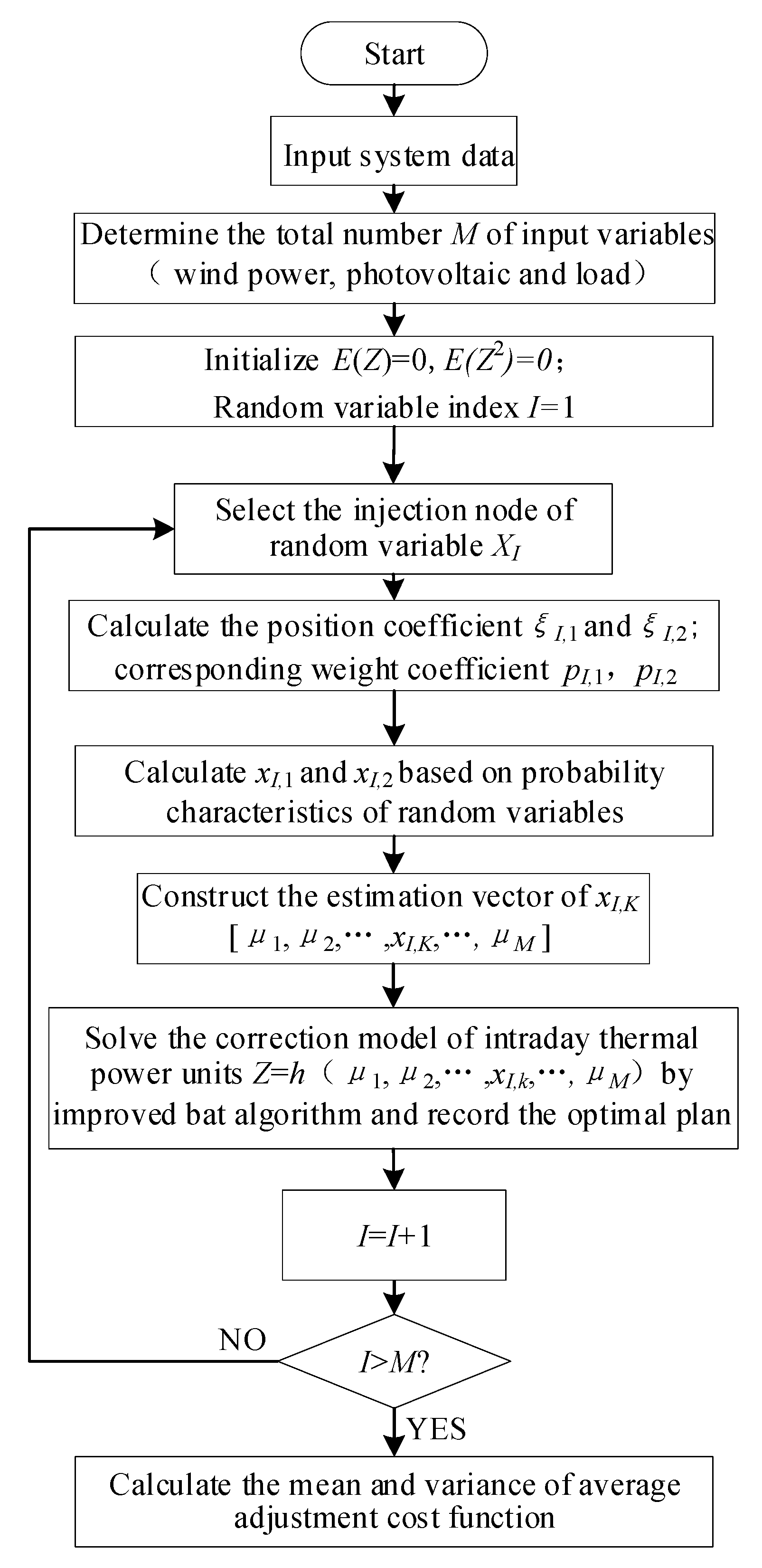
min F = F 1 + t = 1 T [ C tax ( E C , t E D , t ) ] + Δ f
where Δ f is the average adjustment cost. Due to the uncertainty of wind speed, solar radiation, and load demand prediction, this cost caused by intraday thermal power unit plans deviating from the day-ahead scheduling plan.
The demand response cost in the above low-carbon economic dispatching objective function is composed of day-ahead price demand response cost C PDR , t and intraday IDR cost C IDR , t . In addition, it can be expressed as:
f DR = t = 1 T ( C PDR , t + C IDR , t )
The intraday IDR has a certain scheduling cost, which is to give the corresponding economic compensation to the users who adjust the load on demand.
C IDR , t = { d = 1 N IDR ω t ( s IDR , t , d + m t , d + )   Increasing   Load d = 1 N IDR ω t ( s IDR , t , d m t , d )   Decreasing   Load
where ω t is the 0-1 variable, which represents that the virtual unit participates in or not participates in intraday scheduling at time t, N IDR is the number of ladder price segments, s IDR , t , d + and s IDR , t , d are respectively the increase or decrease of electric quantity of the IDR virtual unit when it is in the d-th ladder price at time t, m t , d + and m t , d are the unit cost of increasing or decreasing electric quantity respectively.
To fully mobilize the flexibility of the demand response on the load side and realize the absorption of wind farms and PV stations in the multi-energy cooperative scheduling system. In this paper, the load response of the IDR users will not transfer to other periods, and meets the following constraints:
0 t = 1 T | P IDR , t | P IDR , max
where P IDR , max is the maximum value of IDR in the whole scheduling cycle.

4.3. Solutions

The probabilistic power flow optimization method based on uncertain data is used to solve the day-ahead scheduling plan, and the minimum value of average adjustment cost in the intraday stage is calculated by the deviation power of wind farms, PV stations, and load. To deal with random variables, the two-point estimation method replaces each uncertain value with the value on both sides of the mean, and takes the mean of other uncertain quantities, and then calculate the probability power flow model. Compared with the Monte-Carlo method of random sampling, a two-point estimation method has a smaller calculation amount and higher accuracy, which is used to estimate the average adjustment cost, and the improved bat algorithm is used to solve the random variable optimization model.

4.3.1. Bat Algorithm and Individual Coding

The BA (Bat Algorithm) is widely used in engineering because of its simple parameter setting and understandable principle. In the process of optimization, the position X I , speed v I , pulse frequency f I , pulse volume A I and pulse frequency r I of each bat are assigned randomly. However, this algorithm is easy to converge prematurely, a genetic algorithm is introduced to make the bat individuals have genetic characteristics of GA (Genetic Algorithm), and the relationships between individual bats are enhanced, which is helpful to realize the global search.
The mathematical model of bat algorithm [27] is as follows:
{ f I = f min + ( f max f min ) ω v I t = v I t 1 + ( x I t 1 x * ) f I x I t = x I t 1 + v I t
where f I [ f min , f max ] , ω is the random vector with a range of [0,1], X I t and v I t respectively represent the position coordinate and flight speed of the I-th bat at time t, and X is the optimal solution (i.e., the optimal position coordinate) at the current time.
Position update formula in the bats’ flight process:
x n e w = x o l d + δ A t
where δ [0,1]; A t is the average loudness of bats at time t. When the bat approaches the target, the emission rate r I will increase and the loudness A I will decrease, and the updated formula is as follows:
A I t + 1 = ε A I t , ε [ 0 , 1 ]
r I t + 1 = r I 0 ( 1 e γ t ) , γ > 0
This paper proposes a two stages optimization scheduling model for the wind-PV-thermal-storage system, and the objective function of this model is considered to be bat food and expressed as the random distribution point in space. In addition, the process of searching for food and updating the location of individual bats is the process of finding the optimal generation-load scheduling plan. The number of the objective function indicates whether the location of individual bats is good or bad. After several optimizations, bat individual location keeps approaching the global optimal value of the objective function. In solution space, the algorithm lets bat individual pulse frequency increase and loudness decrease to improve the accuracy of the solution.
The constraints of the joint dispatching system constitute a multidimensional solution space, in which Npop individual bats are generated. Each generation-load dispatching scheme is coded as an individual bat, which can form gene sequences [28]. In addition, each individual bat contains wind power, photovoltaic power, and load information.
X I = [ P W , P PV , P L , P DR ] I = 1 , 2 , N pop
After encoding, genetic algorithm selection, crossover, and mutation are carried out on the individual bats, and the individual information is transmitted to the offspring through encoding.

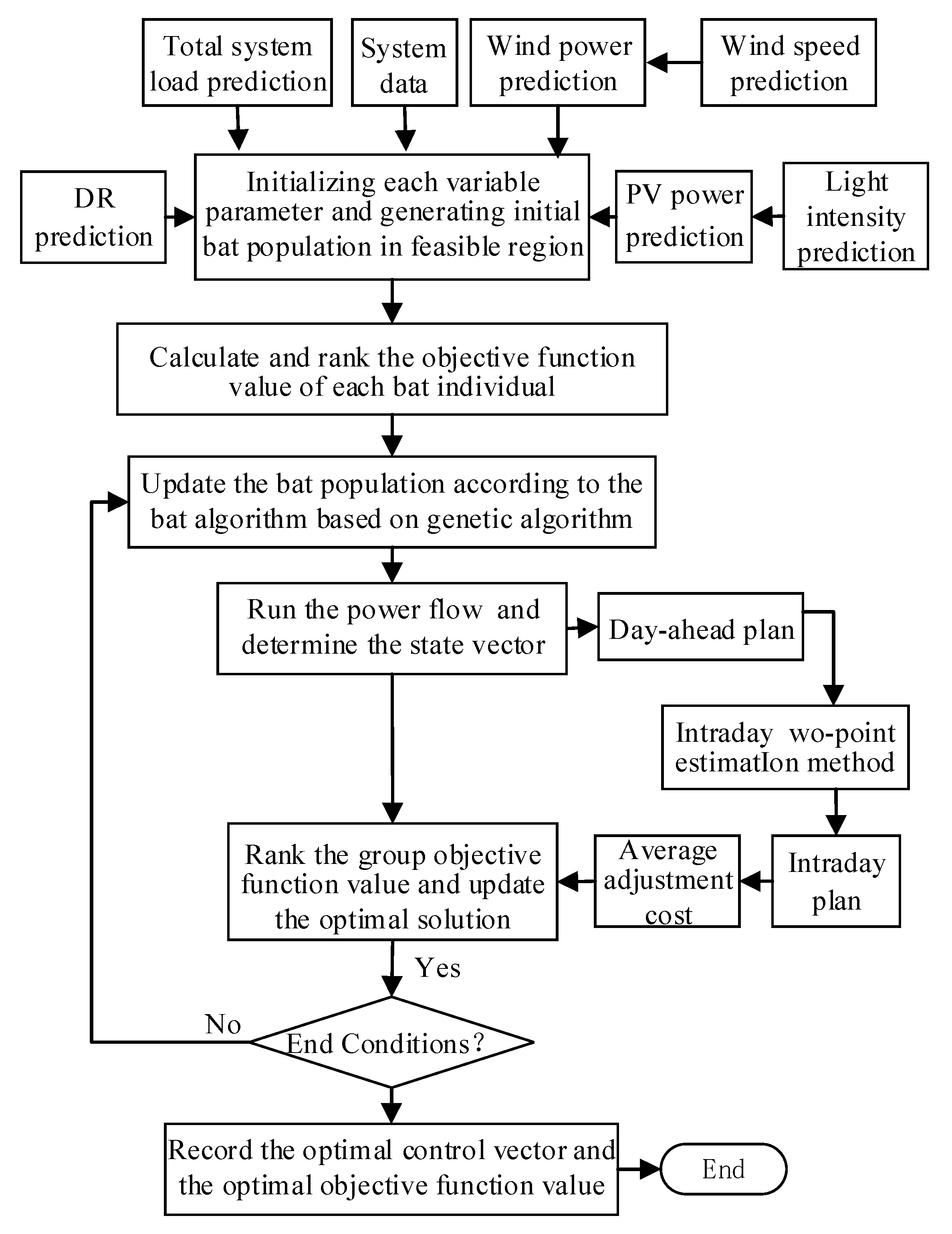
4.3.2. Algorithm Steps

Bat algorithm [29] based on the genetic algorithm is applied to solve the two-stage optimal scheduling model in the wind-PV-thermal-storage system. The algorithm steps are as follows:
Step 1: initialize the algorithm parameters, and generate the gene sequence of the individual bat, in which wind power, photovoltaic power, load, and other parameters are set according to the generation-load uncertainty model. In addition, determine the number of iterations is 1000 and objective function f ( X ) . Set the total number of bats Npop, position X 0 , flight speed v 0 , loudness A 0 , and frequency f 0 .
Step 2: randomly generate Npop bats within the feasible range of control variables as the current optimal solution set, calculate the objective function value of the current bat gene sequence and sequence them from small to large, and retain the first half of the individual bats for update and proliferation.
Step 3: start iterative calculations. Change frequency and update individual speed, and take the new bat population as the parent generation to carry on selection, velocity push average crossover and mutation, and then constitute the first half of the offspring bat population;
Step 4: update the individual location of the parent bat population, and then determine whether the local search condition rand1 > r I is satisfied. If so, the optimal solution is selected for local search to get a new position to replace the original position;
Step 5: determine whether the new fitness value satisfies f ( X I ) < f b e s t and the random number rand2 < A I . If so, the new solution is accepted to form the second half of the offspring bat population, and the function value of the individual bat is updated;
Step 6: rank and evaluate the objective function value of the entire offspring population, and then update the current optimal position (solution) X ;
Step 7: determine whether the maximum number of iterations is exceeded. If so, return step 2. Otherwise, end the algorithm and the optimal value is output.
Figure 3 shows the two-stage optimal scheduling solution flow chart proposed in this paper, including day-ahead scheduling and intraday scheduling. In the day-ahead stage, according to the wind energy, photovoltaic energy, total load of the system and price-type demand response model mentioned above, Monte-Carlo method is used to conduct random sampling, and then the improved bat algorithm is used to solve day-ahead scheduling plan, so as to determine thermal power unit start–stop combination, electricity price in each period and price demand response quantity. In the intraday stage, according to the parameter distribution functions of wind, photovoltaic, and load, a two-point estimation stochastic optimization model is built to calculate the minimum average adjustment cost and determine the output of thermal power units, and the process is shown in Figure 4, and details are analyzed in the Appendix C. Based on this, the improved bat algorithm is used to obtain the IDR quantity and the output of other units.

5. Example Simulation and Analysis

5.1. Different Scheduling Scenarios

According to the scheduling method proposed in this paper, the following five kinds of simulation scheduling scenarios are designed to analyze the impact of the energy storage system, demand response, and carbon cost on absorbing renewable energy power.
Case1: This scene contains wind, solar, and thermal generator units, regardless of battery storage power station, user-side demand response, and cost of carbon treatment.
Case2: Battery energy storage scene, in which a battery storage power station is introduced in Case1, with a capacity of 50 MW and the initial energy storage is 0. The maximum charge and discharge power are 20 MW and the charge and discharge loss is 0.04.
Case3: Generation-load interactive scene, in which the day-ahead price demand response virtual unit and the intraday IDR virtual unit are introduced in Case1. When the user does not participate in the price-type demand response, the electricity price is 71 $/MW∙h, and the load self-elastic coefficient is −0.3 [30].
Case4: Low-carbon scene, in which the carbon cost is introduced based on Case1. For traditional coal-fired units, the CO2 emission cost of unit electricity quantity is 0.88−1.21·t/(MW∙h), and the value in this region is set as 0.798·t/(MW∙h). The carbon treatment price is 17$/t, and other relevant parameters can be found in [31].
Case5: Comprehensive scene, in which battery energy storage power station, demand response, and carbon cost are introduced in Case1. Detailed parameters are the same as above.

5.2. Basic Data

In this paper, a wind-PV-thermal-storage power system of a north city is selected for simulation, which contains 1200 MW thermal power units, 200 MW wind units, and 400 MW photovoltaic units. The error is 20% between the actual active power output and the predicted active power output of wind power and photovoltaic power generation. In addition, their samples follow the Weibull distribution between P max min and P max max , and average adjustment cost can be calculated by a two-point estimation method. According to the uncertain models of wind, solar, and system load, the wind and photovoltaic output are predicted. The predicted curves are shown in Figure 5 and the operation cost coefficients and maintain cost coefficients of wind and photovoltaic generation are shown in Table 1. Combined with the actual situation, the maximum price variation of the day-ahead price demand response virtual unit in this region is to increase or decreased 50%, and the inflection point of the electricity price change rate is ± 0.3 [32]. The critical value and saturated value of intraday IDR virtual units are 40 $ and 55 $ respectively.
In the existing power system, the installed number of thermal power generators is more, and the capacity of energy storage power station is limited. It is a big challenge to face the large-scale new energy connection, and there is a huge peak-valley difference caused by the user’s electricity consumption behavior. Therefore, the number of started thermal power generators is too much during peak hours, but units fail to stop frequently during low hours, and they often run in depth peak load cycling. The operation cost of thermal power plants increases with peak-shaving depth. The standard coal price in calculating operation cost is 85.57 $/t, and the operating parameters of thermal power units are shown in [33]. The start–stop cost and loss cost curves of thermal power units at different peak load adjustment depths are shown in Figure 6. Parameters settings of improved bat algorithm are listed in Table 2.

5.3. Algorithm Testing

To verify the superiority and effectiveness of the improved algorithm, assuming that the actual changes of wind power, photovoltaic power generation, and load are consistent with the forecast. Then the original bat algorithm and the improved bat algorithm are used to solve the day-ahead scheduling model, and the program is independently simulated 30 times. It is important to note that the depth peak state of thermal power unit and demand response is not considered in this power system. The average value and standard deviation of the total system operating cost, and simulation time are shown in Table 3.
According to Table 3, the convergence accuracy of the improved bat algorithm is obviously better than the original algorithm. Incorporating genetic characteristics of genetic algorithms increases the diversity of bat populations, and it can effectively avoid local optimization in the high-dimensional situation and get a global optimum solution quickly.

5.4. Results Analysis

5.4.1. Different Scheduling Scenes Analysis

Energy storage power stations have a strong complementary ability to wind and solar power. Considering the uncertainty of wind power, the thermal power unit and the IDR are adjusted in the intraday scheduling, and the optimization scheduling results of each scheduling scene are analyzed.
Table 4 shows the optimal scheduling costs in different system scenes. In the basic scene, there is no battery energy storage station and demand response, so thermal motor units are often in a deep peak condition and climb frequently. The thermal power unit cost is 262,140 dollars and the average adjustment cost is 81,735 dollars, and they are higher than in other cases. Compared to the day-ahead schedule in Table 3, the total system cost was reduced by $6,144.49. Case 2 contains the battery energy storage station, which relieves the peaking pressure of the thermal power unit to a certain extent, so the thermal power unit output cost and the intraday average adjustment cost are reduced compared with case1. In case3, the demand response virtual unit participates in the scheduling, which reduces the system load uncertainty during the day-ahead and intraday stage, and effectively avoids the impact of load fluctuation on system operation. In case4, the total system cost is 13,249 dollars less than the basic scene. Because this scene includes the carbon treatment cost, the output of thermal power units is limited to achieve low-carbon scheduling, and the data in the table shows that the amount of wind and light waste is reduced. Case5 integrates various factors, and the unit adjustment cost is reduced to $21,362 in the simulation results. Meanwhile, the total system cost is reduced by 14.82% compared with the basic scene. Therefore, the scheduling model proposed in this paper has significant advantages in reducing the two-stage average adjustment cost.
According to the system load curve before and after demand response in Figure 7, the day-ahead electricity price guides residential users to change their electricity consumption behavior and intraday electricity price encourages industrial users to adjust the electricity time, which greatly reduces the peak-valley difference. It is economical and low-carbon to smooth the fluctuation of load, and the power supply pressure on the power side is eased during peak period, and it is obvious that the power interest rate is increased during the valley period. As is shown in Table 4, the adjustment cost and total system cost are reduced effectively with the demand response virtual units.
In Figure 8, the optimal dispatching plan under the comprehensive scene is shown. From 19:00 to 20:00, the photovoltaic station output decreases to 0, and wind power output begins to decline. At this moment, the output of the energy storage station is relatively large, and the thermal power unit is an upward climbing state. From 22:00 to 24:00, the system load decreases continuously. In addition, thermal power units change into a downward climbing state, and the output of the energy storage power station gradually decreases. It can be seen from the figure that using the complementary characteristics of multiple generations can be used to promote the economic and low-carbon dispatching for the collaborative dispatching power system.

5.4.2. The Effect of Uncertainty on Scheduling Results

This paper mentions the uncertainty model of wind power, photovoltaic power, system load, and demand response. These uncertainties’ influence on system optimization results is analyzed under five cases, and the maximum prediction error of wind power, photovoltaic power and system load is increased by 30%. The prediction error of the virtual response unit (including day-ahead PDR and intraday IDR) increases by 30%, and other conditions remain the same. The average adjustment cost and total system cost under each scene can be simulated, as shown in Table 5.
Compared with Table 4 and Table 5, the total system cost in each scheduling scene increases by 10.1%, 7.33%, 5.08%, 8.73%, and 3.51%, respectively. It is obvious that the total system cost of the two-stage optimal scheduling model increases with the prediction error. Comparing the basic scene and synthetic scene, two-stage scheduling of wind, solar, thermal, and storage systems with demand response have a proportional increase in total system costs with the prediction, but the increase is minimal. Meanwhile, the unit adjustment cost is relatively lower. It is shown that the proposed model is better than other models in dealing with prediction errors. With economic dispatching as the objective function, the prediction error of wind power and photovoltaic power is kept 20% to study the effect of load prediction. The change curve of integrated scene system operation cost under different load prediction errors is shown in Figure 9. It can be seen from the figure that the total system cost increases with the load prediction error. The reason is that to ensure the safe and stable operation of the power system, the number of thermal power units is increased during the peak load period to meet the power demand. In the valley period, thermal power units may run in low load conditions, in which the operating cost is higher. However, compared with the traditional scheduling method (Case1), the two-stage optimal scheduling method (Case5) proposed in this paper is less affected by the load prediction error, which indicates that the ability of power system to deal with the prediction error can be improved by the addition of source-load interaction in the day-ahead and intraday stages.

6. Conclusions

Facing the current situation of large-scale renewable energy integration, this paper considers the uncertainty of wind power, photovoltaic, load, and demand response virtual units in different time scales, and the depth peak regulation characteristics of the thermal power unit. In addition, then a low-carbon economic scheduling model with day-ahead and intraday stage is built for wind, solar, and thermal storage power systems. The validity of this model is verified by examples. The conclusions are as follows:
(1) For wind, solar, thermal power, and storage systems, the two-stage coordination scheduling model including day-ahead and intraday is proposed in this paper, which is less affected by the uncertainty of wind, solar, load, and demand response than the day-ahead scheduling model. In the simulation results, the total system cost is reduced by 16.2% compared with the day-ahead scheduling method. This scheduling model has a significant advantage in reducing the total system cost.
(2) Based on the response of PDR and the IDR virtual unit in the day-ahead and intraday stage, the carbon processing cost is introduced into the economic dispatch model, which is effective to achieve low-carbon economic dispatch of the power system. The introduction of demand response can adjust the power consumption time of users to some extent, and the source-load interaction can greatly reduce the limited power generation cost of renewable energy.
(3) Considering the normal operation state and deep peak regulation state of thermal power units, the generation cost of thermal power units is quantified when large-scale wind power and PV power is incorporated into the grid, so that the model can reflect the actual working conditions more authentically. With the increase of peak regulation depth, the start–stop frequency of thermal power units decreases, and it is conducive to absorbing the intermittency and volatility of renewable energy power generation.
With the change of electricity price mechanism and market mechanism, the power system dispatching method proposed in this paper will have a great application prospect in absorbing large-scale renewable energy generation. The next step is to study the influence of the correlation between wind power and PV power generation on day-ahead and intraday scheduling of wind, solar, thermal power, and storage systems with demand response.

Author Contributions

X.K. and S.Q. conceived the idea of the study and conducted the research. X.K., S.Q. and F.S. analyzed most of the data and wrote the initial draft of the paper. Z.C., X.W., and Z.Z. provided data for the study and contributed to finalizing this paper. All authors have read and agreed to the published version of the manuscript.

Funding

This research was funded by the Open Fund of State Key Laboratory of Power Grid Safety and Energy Conservation (China Electric Power Research Institute) (No. JBB51201801311).

Conflicts of Interest

The authors declare no conflicts of interest.

Appendix A

In this paper, the Weibull probability density function is adopted to express the light intensity:
f ( R ) = ω ( K 1 C 1 ) ( R C 1 ) K 1 1 exp [ ( R C 1 ) K 1 ] + ( 1 ω ) ( K 1 C 2 ) ( R C 2 ) K 2 1 exp [ ( R C 2 ) K 2 ] 0 < R <
where ω is the weight parameter within the range of 0 ~ 1 (0 < ω < 1). K1, K2, C1, and C2 are shape factors and scale factors of a photovoltaic panel, respectively.
The wind turbine power distribution can be expressed as:
f ( v ) = ( K 3 C ) ( v C ) K 3 1 exp [ ( v C ) K 3 ]
where v is wind speed, m/s, K 3 is shape factor, and C is the scale parameter.
The uncertain model of the system load is:
f L ( l ) = 1 σ L 2 π × exp [ ( ( l μ L ) 2 2 σ L 2 ) ]
where l is system load, μ L and σ L are the mean and standard deviation of uncertain loads respectively.

Appendix B

The power of battery storage station meets the following requirements:
0 P B , c P B , c , max
0 P B P B , max
where P B , c and P B are respectively charge-discharge power of energy storage station, P B , c , max and P B , max represents the maximum charge-discharge power.
The power balance and power constraints of the energy storage power station are as follows:
W B ,   t + 1 = W B , t + P B , t Δ t
W B , min W B , t W B , max
where W B , min , W B , max are the minimum and maximum residual power of the battery storage power station respectively. W B , t is the residual power of the energy storage power station in the time period t.

Appendix C

The change curve of wind power, PV power, and load can be simulated by Weibull distribution and normal distribution. In the intraday stage, the wind farm, solar station, and load have random characteristics. Therefore, the two-point estimation method is used to deal with this uncertainty, in which each uncertainty variable is replaced with the deterministic value on both sides of the node mean, and the deterministic power flow is calculated. In form, this calculation can be regarded as a multivariate nonlinear function:
Z = h ( X )
where X is a random input vector, which is used to describe the wind power output, photovoltaic power output, and load, and Z is the output variable, which represents the intraday adjustment cost of thermal power unit relative to the day-ahead scheduling plan.
X = [ X 1 , X 2 , X 3 , , X M ]
where M is the dimension of a random variable, which is determined by the number of wind power units, photovoltaic units, and loads. The estimated information of each random variable consists of a group ( x I , K , p I , K ) , I = 1,2…,M, K = 1,2, and x I , K is estimated point, and the corresponding estimate vector is [ μ X , 1 , μ X , 2 , x I , K , , μ X , M ] , p I , K is the corresponding weight. The variables Z ( I , K ) = h ( μ X , 1 , μ X , 2 , x I , K , , μ X , M ) are evaluated by the optimization algorithm and all the estimated points are calculated successively. Finally, the statistical information of the desired variables can be obtained.
Given the probability distribution of random variables, the two-point estimation method is used to evaluate the probability distribution function of average adjustment cost Z . The specific steps are as follows:
Step 1: input system data, including branch parameters, transformer ratio, and other deterministic data, as well as the expectation and generation-load distribution function, and determine the number M of uncertain variables.
Step 2: initialize I = 1 ; E ( Z ) = 0 ; E ( Z 2 ) = 0 .
Step 3: select the random variable of node injection X I , and determine the position coefficient ξ I , 1 and ξ I , 2 , and probability concentration p I , 1 and p I , 2 .
{ ξ I , 1 = m ξ I , 2 = m p I , 1 = p I , 2 = 1 2 m
Step 4: calculate the X I , 1 and X I , 2 of estimated distribution points on both sides of the mean value;
{ X I , 1 = μ X , I + ξ I , 1 σ X , I X I , 2 = μ X , I + ξ I , 2 σ X , I
where μ X , I and σ X , I are the mean and standard deviation of random quantities respectively.
Step 5: the improved bat algorithm is adopted to calculate deterministic power flow optimization for random variables X I , K (K = 1,2), and the average adjustment cost in each period of each estimation point can be obtained.
X = [ μ X , 1 , μ X , 2 , , x I , K , , μ X , M ]
Step 7: update E ( Z ) and E ( Z 2 ) .
E ( Z ) I = 1 M K = 1 2 ( P I , K h ( [ μ X , 1 , μ X , 2 , , X I , K , , μ X , M ] ) )
E ( Z 2 ) I = 1 M K = 1 2 ( P I , K h ( [ μ X , 1 , μ X , 2 , , X I , K , , μ X , M ] ) 2 )
Step 7: repeat from step 3 to step 6, I = I + 1 and loop over the variables.
Step 8: calculate the mean and standard deviation:
μ Z = E ( Z )
σ Z = E ( Z 2 ) μ Z 2

References

  1. Li, X.; Zhang, R.F.; Bai, L.Q. Stochastic low-carbon scheduling with carbon capture power plants and coupon-based demand response. Appl. Energy 2018, 210, 1219–1228. [Google Scholar] [CrossRef]
  2. Hemmati, R.; Saboori, H.; Jirdehi, M.A. Stochastic planning and scheduling of energy storage systems for congestion management in electric power systems including renewable energy resources. Energy 2017, 133, 380–387. [Google Scholar] [CrossRef]
  3. Shen, J.J.; Cao, R.; Su, C.J. Big data platform architecture and key techniques of power generation scheduling for hydro-thermal-wind-solar hybrid system. Proc. CSEE 2019, 39, 43–55. [Google Scholar]
  4. Dui, X.W.; Zhu, G.P.; Yao, L.Z. Two-stage optimization of battery energy storage capacity to decrease wind power curtailment in grid-connected wind farms. IEEE Trans. Power Syst. 2018, 33, 3296–3305. [Google Scholar] [CrossRef]
  5. An, L.; Wang, M.B.; Qi, X. Optimal dispatching of multi-power sources containing wind/photovoltaic/thermal/hydro-pumped and battery storage. Renew. Energy Res. 2018, 33, 1492–1498. [Google Scholar]
  6. Reddy, S.S.; Vuddanti, S.; Babu, B.C.; Jung, C. Multi-objective based optimal generation scheduling considering wind and solar energy systems. Int. J. Emerg. Electr. Power Syst. 2018, 19, 1553–1779X. [Google Scholar]
  7. Reddy, S.S. Optimal scheduling of thermal-wind-solar power system with storage. Renew. Energy 2017, 101, 1357–1368. [Google Scholar] [CrossRef]
  8. Eissa, M.M. First time real time incentive demand response program in smart grid with “i-Energy” management system with different resources. Appl. Energy 2018, 212, 607–621. [Google Scholar] [CrossRef]
  9. Zhang, M.L.; Ai, X.M.; Fang, J.K. A systematic approach for the joint dispatch of energy and reserve incorporating demand response. Appl. Energy 2018, 230, 1279–1291. [Google Scholar] [CrossRef]
  10. Mohammad, N.; Yateendra, M. Coordination of wind generation and demand response to minimise operation cost in day-ahead electricity markets using bi-level optimization framework. IET Gener. Transm. Distrib. 2018, 22, 3793–3802. [Google Scholar] [CrossRef]
  11. Geng, K.L.; Ai, X.; Liu, B. A Two-Stage Scheduling Optimization Model and Corresponding Solving Algorithm for Power Grid Containing Wind Farm and Energy Storage System Considering Demand Response. In Proceedings of the International Conference on Applied Mechanics and Mechanical Automation (AMMA), Hong Kong, China, 22–24 June 2017; pp. 139–145. [Google Scholar]
  12. Sun, Y.J.; Wang, Y.; Wang, B.B. Multi-time scale decision method for source-load interaction considering demand response uncertainty. Autom. Electr. Power Syst. 2018, 42, 106–113. [Google Scholar]
  13. Najafi, G.A.; Pashaei, F.A.; Sayyad, N. A stochastic self-scheduling program for compressed air energy storage (CAES) of renewable energy sources (RESs) based on a demand response mechanism. Energy Convers. Manag. 2016, 120, 388–396. [Google Scholar]
  14. Zhang, Y.C.; Liu, K.P.; Liao, X.B. Multi-time scale source-load coordination dispatch model for power system with large-scale wind power. High Volt. Eng. 2019, 45, 600–608. [Google Scholar]
  15. Liu, J.C.; Wen, Z.G. An optimal scheduling method to hybrid wind-solar-hydro power generation system with data center in demand side. Power Syst. Technol. 2019, 43, 2449–2460. [Google Scholar]
  16. Ju, L.W.; Yu, C.; Tan, Z.F. A two-stage scheduling optimization model and corresponding solving algorithm for power grid containing wind farm and energy storage system considering demand response. Power Syst. Technol. 2015, 39, 1287–1293. [Google Scholar]
  17. Lin, L.; Zou, Q.L.; Zhou, P. Multi-angle economic analysis on deep peak regulation of thermal units with large-scale wind power integration. Autom. Electr. Power Syst. 2017, 41, 21–27. [Google Scholar]
  18. Lu, R.Z.; Ding, T.; Qin, B.Y.; Ma, J.; Bo, R.; Zhao, Y.D. Reliability based min-max regret stochastic optimization model for capacity market with renewable energy and practice in China. IEEE Trans. Sustain. Energy 2018, 10, 2065–2074. [Google Scholar] [CrossRef]
  19. Lu, R.Z.; Ding, T.; Qin, B.Y.; Ma, J.; Dong, Z.Y. Multi-Stage Stochastic Programming to Joint Economic Dispatch for Energy and Reserve with Uncertain Renewable Energy. IEEE Trans. Sustain. Energy 2019, 1. [Google Scholar] [CrossRef]
  20. Luo, C.J.; Li, Y.W.; Xu, H.P. Influence of demand response uncertainty on day-ahead optimization. Autom. Electr. Power Syst. 2017, 41, 22–29. [Google Scholar]
  21. Liu, B.D.; Zhao, R.Q.; Wang, G. Uncertainty Programming with Application; Tsinghua University Press: Beijing, China, 2003; pp. 213–217. [Google Scholar]
  22. Li, Y.R. Modeling of Demand Response Considering the Uncertainty and Its Applications in Power System Operation. Master’s Thesis, Southeast University, Nanjing, China, 2015. [Google Scholar]
  23. Che, Q.H.; Wu, Y.W.; Zhu, Z.G. Carbon trading based optimal scheduling of hybrid energy storage in power systems with large-scale photovoltaic power generation. Autom. Electr. Power Syst. 2019, 43, 76–82. [Google Scholar]
  24. Liu, X.D.; Chen, H.Y.; Yao, C. Economic dispatch considering deep peak-regulation and interruptible loads for power system incorporated with wind farms. Electr. Power Autom. Equip. 2019, 32, 95–99. [Google Scholar]
  25. Cui, Y.; Yang, Z.W.; Zhong, W.Z. A joint scheduling strategy of CHP with thermal energy storage and wind power to reduce sulfur and nitrate emission. Power Syst. Technol. 2018, 42, 1063–1070. [Google Scholar]
  26. Kong, X.Y.; Xiao, J.; Wang, C.S.; Cui, K.; Jin, Q.; Kong, D. Bi-level multi-time scale scheduling method based on bidding for multi-operator virtual power plant. Appl. Energy 2019, 249, 178–189. [Google Scholar] [CrossRef]
  27. Niknam, T.; Azizipanah-Abarghooee, R.; Zare, M.; Bahmani-Firouzi, B. Reserve constrained dynamic environmental/economic dispatch: A new multi-objective self-adaptive learning bat algorithm. IEEE Syst. J. 2013, 7, 763–776. [Google Scholar] [CrossRef]
  28. Guo, D.D.; Song, J.G.; Wang, X.Z. Research on indoor coverage optimization strategy of electric wireless private network based on improved bat algorithm. Distrib. Util. 2019, 36, 23–28. [Google Scholar]
  29. Wang, T. Bat Algorithm Based on Hybrid Strategy. Master’s Thesis, Department of Software Engineering Guangxi University, Guangxi, China, 2015. [Google Scholar]
  30. Bie, Z.H.; Hu, G.W.; Xie, H.P.; Li, G.F. Optimal dispatch for wind power integrated systems considering demand response. Autom. Electr. Power Syst. 2014, 38, 115–120. [Google Scholar]
  31. Zhang, G.; Zhang, F.; Zhang, L. Two-stage robust optimization model of day-ahead scheduling considering carbon emissions trading. Proc. CSEE 2018, 38, 5490–5499. [Google Scholar]
  32. Song, Y.H.; Tan, Z.F.; Li, H.H. An optimization model combining generation side and energy storage system with demand side to promote accommodation of wind power. Power Syst. Technol. 2014, 38, 610–615. [Google Scholar]
  33. Dong, C.; Zhang, Y.T.; Liu, J.N.; Wu, B.X. Real-time generation scheduling model and its application considering deep peak regulation of thermal power units. Electr. Power Autom. Equip. 2018, 39, 108–113. [Google Scholar]
Figure 1. Wind-PV-thermal-storage scheduling mode considering demand response.
Applsci 10 00971 g001
Figure 2. IDR curve.
Applsci 10 00971 g002
Figure 3. Two-stage optimal scheduling solution flow chart.
Applsci 10 00971 g003
Figure 4. Flow chart based on the two-point estimation method.
Applsci 10 00971 g004
Figure 5. Wind and PV forecast output curve and system load forecast curve.
Applsci 10 00971 g005
Figure 6. Start–stop cost and loss cost curves of thermal power units at different peak load adjustment depths.
Applsci 10 00971 g006
Figure 7. System load curve before and after demand response.
Applsci 10 00971 g007
Figure 8. The optimal scheduling plan in case 5.
Applsci 10 00971 g008
Figure 9. The change curve of integrated scene system operation cost under different load prediction errors.
Applsci 10 00971 g009
Table 1. Operation Cost Coefficient and Maintenance Cost Coefficient of Wind Power and PV Power Generation.
SymbolCapacity (MW)Cost Coefficient ($/MW∙h)
Wind Power453.25
PV403.5
Table 2. Improved BA parameter initialization settings.
SymbolParameter ValueSymbolParameter Value
N pop 100 γ 0.05
f I [0,100] A 0 0.25
r 0 0.5 ε 0.95
Table 3. Performance comparison of BA and improved BA.
AlgorithmAverage/$Standard DeviationSimulation Time
BA409,459.884.27192.04
GA396,102.313.24812.43
Improved BA389,024.491.96252.96
Table 4. Optimal scheduling costs in different system scenarios.
Cost/$Case1Case2Case3Case4Case5
Thermal262,140257,343147,004237,406139,512
Storage-14,828--16,871
DR--109118-118356
Adjustment81,73560,13842,03173,02121,362
Limit39,00536,71018,49359,20430,048
Total38,2880369,019316,646369,631326,149
Table 5. System optimal scheduling with an uncertainty of 30%.
Cost/$Case1Case2Case3Case4Case5
Adjustment87,12065,02445,31778,35223,824
Total421,551396,069332,716401,899337,597

