A High-Performance Deep Learning Algorithm for the Automated Optical Inspection of Laser Welding

Abstract

The battery industry has been growing fast because of strong demand from electric vehicle and power storage applications.Laser welding is a key process in battery manufacturing. To control the production quality, the industry has a great desire for defect inspection of automated laser welding. Recently, Convolutional Neural Networks (CNNs) have been applied with great success for detection, recognition, and classification. In this paper, using transfer learning theory and pre-training approach in Visual Geometry Group (VGG) model, we proposed the optimized VGG model to improve the efficiency of defect classification. Our model was applied on an industrial computer with images taken from a battery manufacturing production line and achieved a testing accuracy of 99.87%. The main contributions of this study are as follows: (1) Proved that the optimized VGG model, which was trained on a large image database, can be used for the defect classification of laser welding. (2) Demonstrated that the pre-trained VGG model has small model size, lower fault positive rate, shorter training time, and prediction time; so, it is more suitable for quality inspection in an industrial environment. Additionally, we visualized the convolutional layer and max-pooling layer to make it easy to view and optimize the model.

1. Introduction

With the rapid development of battery electric vehicles (BEVs), laser welding technology has been widely used in the assembling process of lithium-ion batteries. The performance of BEVs depends highly on the power and energy capacities of their batteries. To meet the desired power and capacity demand for BEVs, a lithium-ion battery pack is assembled from lots of battery cells, sometimes several hundred or even thousands, which depends on the cell configuration and pack size [1]. Several cells are typically joined together to form a module with common bus-bars, and tens of modules are then assembled into a battery pack [2]. As laser welding defects on the safety vent of a battery may cause overheating or explosion over time when it is in use, the quality control of laser welding is very critical, which helps to prolong the life of the batteries and ensure the safety of the batteries. At present, the main methods to detect the quality of welding include laser [3], ultrasonic [4], X-ray [5,6], machine vision [7,8], and so on, which have been widely used by many companies to inspect welding quality during manufacturing. Benefiting from the development of image processing algorithms and camera technology, machine vision is playing a significant role in modern industries for real-time quality assurance [7]. Automated optical inspection (AOI), also called machine vision inspection, is used broadly in solder joint quality inspection [8].

One of the earliest studies on solder joint quality inspection was conducted by Besl and Jain, and they proved that features inferred from facets and Gaussian curvature were better in the classification of a solder joint using a minimum-distance classification algorithm [9]. However, the results were poor for the algorithm’s sensitivity to the illumination environment. Other AOI inspection algorithms are available, such as the defect model through statistical modeling [10], feature map analysis [11], and Gaussian mixture model [12]. However, these algorithms are complex when analyzing the details of the defect images [13]. Some AOI applies Bayes and support vector machine (SVM) to classify defects, and extracts feature information from a feature extraction region. For example, Yun et al. created a method using SVM [14], Wu et al. used the Bayes classifier and an SVM [7], and Hongwei et al. used adaptive boosting (AdaBoosting) and a decision tree [15]. However, note that the feature extraction of the aforementioned methods [7,8,9,10,11,12,13,14,15] is usually set manually by an operator [16]. If the features of numerous components are manually set from the feature extraction region, the efficiency of the AOI process will decrease greatly. Additionally, these methods are easily influenced by the illumination environment.

In our case, namely, the welding defect inspection of battery’s safety vent, the main difficulty encountered by visual inspection algorithms is that the quality of the photographs is seriously affected by the illumination environment [8]. Additionally, the diversity and complexity of welding defects make it difficult to identify a suitable algorithm. Even in one sample, there may be several different defects. These problems can also lead to a high fault positive rate, which is defined as the ratio of the number of defect products categorized as positive to the total number of defect products (regardless of classification). Hence, surface welding defects of safety vent are mainly detected manually in the factory. Recently, deep learning has advanced dramatically in visual object recognition, object detection, and other domains; consequently, it has the potential ability to help to execute defect inspection of safety vent’s surface welding. Compared with the aforementioned methods (such as SVM and AdaBoosting), deep learning allows computational models that are composed of multiple processing layers to learn representations of data with multiple levels of abstraction and to automatically discover representations required for detection or classification [17]. As a key technology in deep learning, CNNs have achieved great success in image recognition and classification [18]. Particularly, CNN architectures have proven to be very efficient and accurate methods in every year’s ImageNet Large-Scale Visual Recognition Challenge (ILSVRC) since 2012 [18,19]. However, CNNs’ effectiveness and accuracy typically depend on large image databases, GPUs, and large-scale distributed clusters, etc., which increase the cost of products in turn.

In our lithium-ion battery laser welding system, the accuracy of safety vent’s welding defect inspection and classification directly affects the value of AOI, which aims to replace human inspection. Therefore, we developed a deep learning algorithm to improve the recognition accuracy of welding quality inspection and defect classification. In this study, based on VGG model, we performed optimization and applied transfer learning theory to restructure the model. The optimized model used a pre-training method to train the network using over 8000 training images on an industrial computer. The testing accuracy rate of 99.87% was achieved for identifying qualified product and defective product, namely the Q-D two-classifications. The training process only took approximately one hour, and it took only 40 ms to predict one image. Additionally, the image of a safety vent was visualized in the convolution layer and max-pooling layer to make it easy to view and optimize the model.

2. Welding Area Image Acquisition and Defect Classification

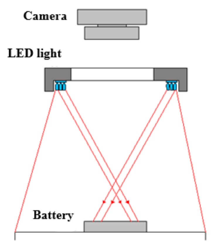
2.1. Welding Area Image Acquisition

In the laser welding AOI system, the welding area images were obtained using a CMOS digital camera (BASLER Basler acA2500-14um camera and UTRON HS2514J lens), and a white annular LED light source (OPT-RI7030) with the brightness of 0-255 levels, as shown in Figure 1. Although most recent AOI systems use a CCD camera, which is more expensive than the CMOS camera [20], the CMOS camera is currently used widely in industrial inspection and possesses quite good image quality [21]. The CMOS digital camera used in this research had 5 megapixels, and it yielded a good resolution of the welding area. Therefore, the 3D shape information of the welding area could be described clearly by a two-dimensional (2D) grey image [10]. A white annular light source was set to be applied to the object at approximately 90 degrees, which made the welded part in the image clearer. When working, the white LED light beams were applied on the battery surface and then reflected into the camera. As deep learning requires diversified samples to best simulate real application scenes, we manage to build such case samples during the process of image acquisition. We collected images three times in total. We used several shooting distances, which varied approximately from 40 cm to 50 cm. Additionally, we randomly changed the brightness of the light sources from bright to dark, and the brightness level was approximately from 50 to 150. Using these approaches, the images captured each time were essentially even, and had different brightness and welding area sizes; hence, they fulfilled the requirement of the deep learning algorithm. Using a white annular light source instead of three LED lights of different colors (red, green, and blue) [7,10,13], the proposed algorithm reduced the requirement for the illumination condition; thus, it is convenient to be used in industrial environments and can reduce the dependence on LED light.

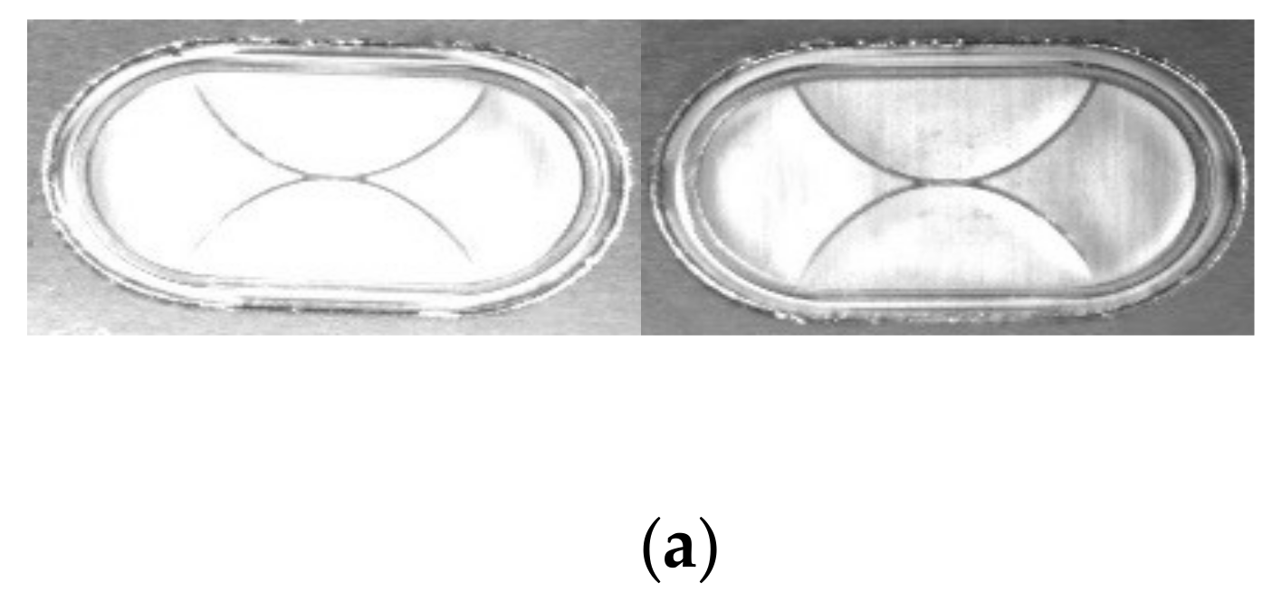
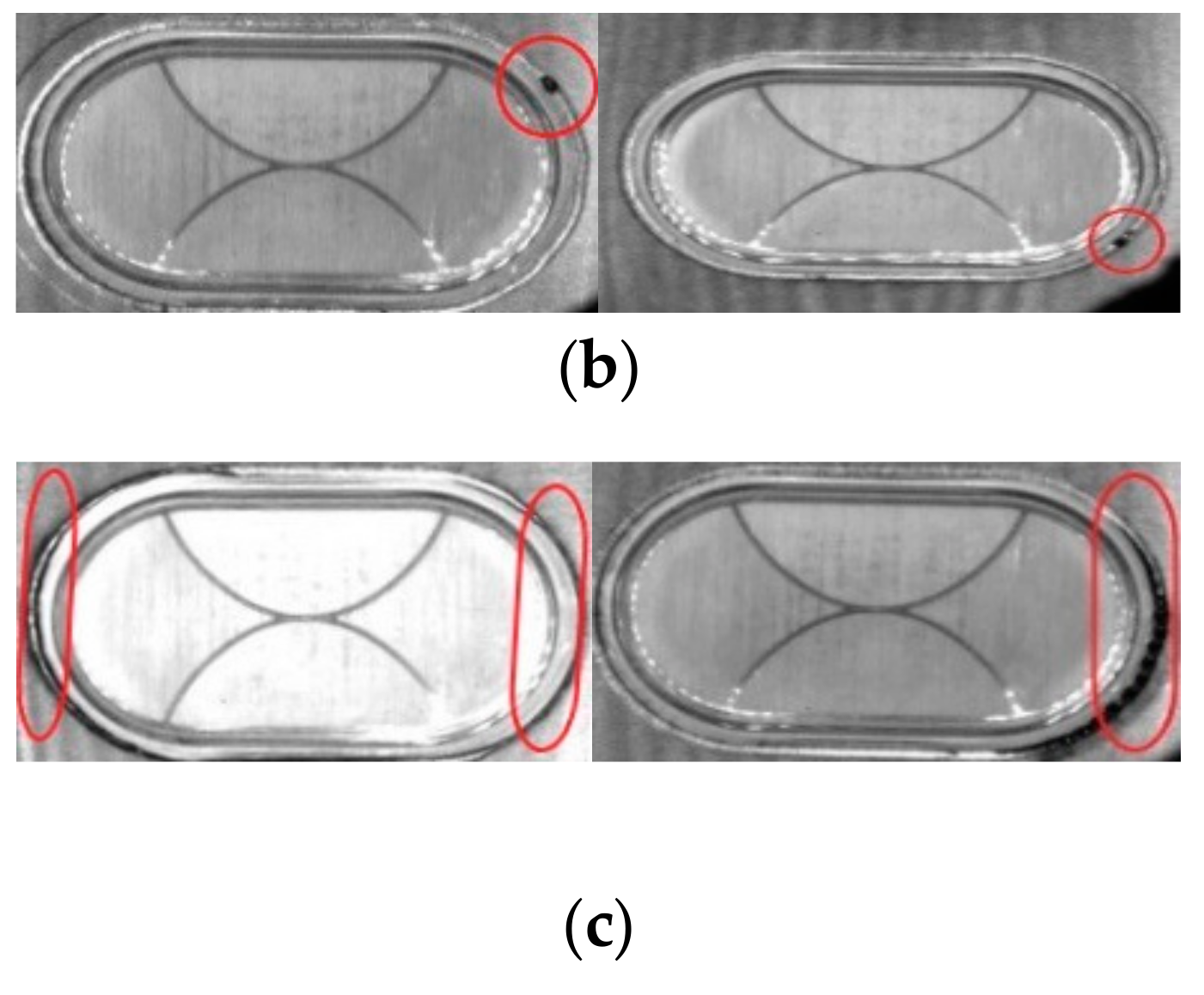
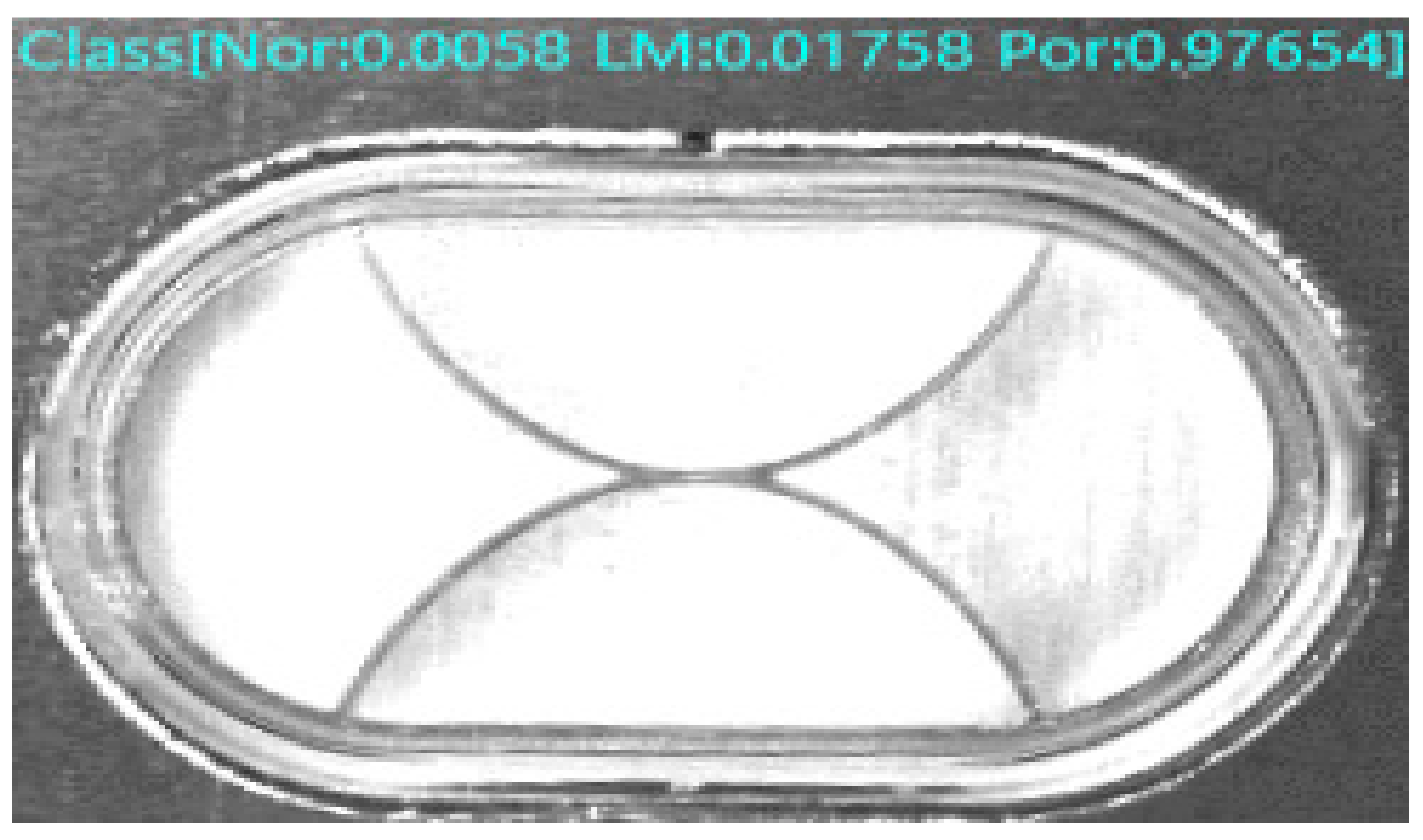
2.2. Defect Classification of the Safety Vent

The defect classification of the safety vent’s welding area focuses on three categories: Two of the most common defect types and one normal type. All data are from a real production floor, as shown in Figure 2. The Normal type refers to a welding area that has no defect. The Porosity defect type refers to a void (the radius is approximately 1 mm) in the welding area. The Level Misalignment defect type occurs when the heights of the two pieces of metal welded are not well aligned (the height difference is approximately 1 mm). The Normal type images represent qualified products and the other two categories represent defective products. Each image was taken from the surface of each individual safety vent. A total of 8941 images were obtained, which consisted of 1715 Normal images, 3879 Porosity images, and 3347 Level Misalignment images. Generally, the welding area images were similar in most of the areas, but each defect type had unique characteristics. For example, the Porosity type typically had a hole in the welding seam, but the position of the hole is uncertain. Except for the black holes in Figure 2b, there was almost no difference in appearance between the Porosity images and Normal images. Additionally, the Level Misalignment type could also have this type of black hole; that is, these classifications are not strictly defined. Taking into consideration this complicated scenario, it is difficult to set a template for inspection using a feature extraction algorithm.

3. Optimized Visual Geometry Group Model

In this section, an optimized CNN model is proposed to classify the welding area defect images, which is based on the Visual Geometry Group (VGG) model. It is worth mentioning that the VGG model achieved first and second places in the localization task and classification task, respectively, in ILSVRC-2014 [19]. A challenging problem for the CNN model is overfitting, which occurs when using small databases [22]. For a big database, because numerous training examples are available, the fundamental characteristics of deep learning can be easily attained. Additionally, deep learning can find interesting features in the training dataset on its own, without any manual operation by a feature engineer. For a small database, overfitting is more likely to occur if there are insufficient diverse samples, particularly when the input samples are images with very high dimensions.

However, exactly how many samples are required is unknown, and depends on the size and depth of the CNN model to be trained. It is impossible to train a CNN model to process a complex visual case with only tens of samples, but a few hundred samples could potentially be sufficient if the CNN model is small and well regularized, and the task is not very complex. Because the CNN model learns local, translation-invariant features, it is highly data efficient for processing the classification case. Training a CNN model from scratch on a very small image dataset will still produce reasonable results despite a relative lack of data. Another advantage of the CNN model is that it can be used repeatedly; that is, an image classification model trained on a large-scale dataset can be reused on noticeably different scenes with only a few changes. Particularly in the computer vision field, many pre-trained models (often trained on a large dataset) can be used to bootstrap powerful vision models on a small dataset.

In this paper, we adopt a pre-trained neural network, which is a saved model formerly trained on ImageNet (a big database) to overcome the overfitting problem. The optimized CNN model is based on the theory of transfer learning. Because ImageNet is a large and generic database, the feature information learned through the pre-trained network can be repurposed in a generic model to resolve novel general tasks [23].

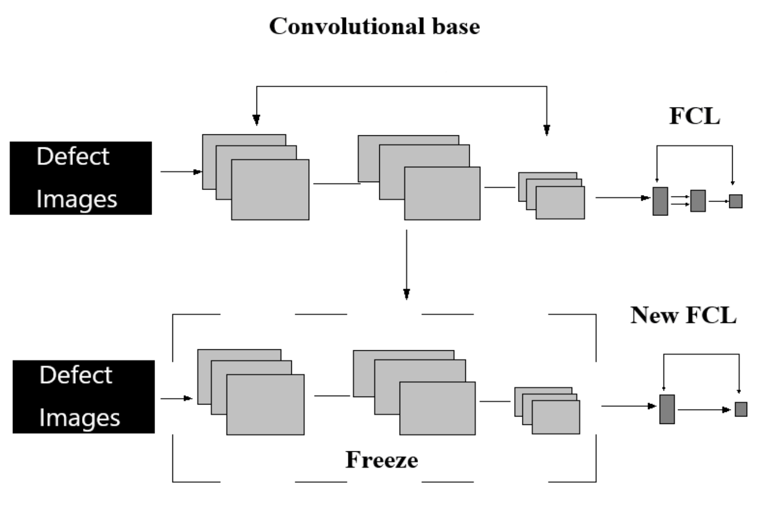
3.1. CNN Architecture

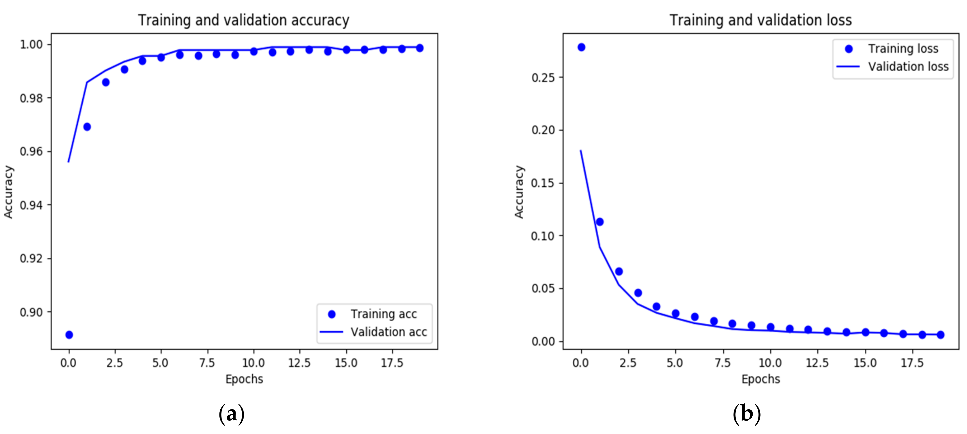
The optimized CNN model has a VGG-16 convolutional base (conv_base) [19] and two fully connected (FC) layers, with the FC layers reconstructed, as shown in

Table 1. Architecture and configuration of the optimized VGG-16 model.

Input (150*150 Grey Image) (New)
VGG-16 conv_base
FC-256 (new)
FC-N (new)
soft-max

. In the training process, images input into the CNN model are resized to 150×150 grey images and do not need any preprocessing. Then, the image passes through a VGG-16 conv_base, which has 14,714,688 parameters previously saved after training in ImageNet. After that, there are two FC layers.

In this study, we remold and retrain the VGG-16 model for welding area quality inspection. We keep the convolutional layers of VGG-16 unchanged and replace the three FC layers with two new FC layers based on the theory of transfer learning. The convolutional layers include a large number of parameters and weights trained in ImageNet. They also have a strong ability to extract features of image edges and contours [24]. The optimized CNN architecture is capable of extracting welding area features distinctively and robustly because the neural network is sufficiently deep. Moreover, it is less likely to overfit. The first FC layer, with 256 channels, is followed by a dropout layer, which is used to decrease overfitting. Regarding the activation function, rectified linear units (ReLUs) are at a potential disadvantage during optimization because the gradient is zero whether the unit is active or not, and this leads to the scenario in which a unit never activates. Like the vanishing gradient problem, we might expect learning to be slow when training ReLU networks with constant zero gradients. Hence, in our experiment, we replace the ReLU activation function with Leaky Rectified Linear Unit (Leaky_ReLU) [25] in the FC layers to solve this problem.

Particularly, the last FC layer of this optimized model represents an N classes predictor, where N is the number of labels in the database [19]. In our case, the last FC layer has two or three channels to represent three-classifications of welding area image mentioned in Section 2.2, and the Q-D two-classifications, respectively. The final layer is the softmax layer, which is used to provide the final classification results. Specifically, softmax is a generalization of the logistic function that maps a length-p vector of real values to a length-K vector of values. Cross-entropy loss together with softmax used in this optimized model is arguably one of the most commonly used supervision components in CNNs. Despite its simplicity, softmax has high popularity and excellent performance in terms of the discriminative learning of features [26].

3.2. Training

The optimized model is trained using the root mean square prop (RMSProp) optimization algorithm with a batch size of 20 examples. RMSProp optimization algorithm is an adaptive learning rate method proposed by Geoff Hinton in 2012 [27]. It has been proven to be effective and has become popular in the deep learning field. In this study, the learning rate is set to 2 × e⁻⁵. Additionally, the dropout rate of 0.5 is used to regularize the first FC layer and reduce overfitting.

As shown in Figure 3, to prevent the convolutional layers’ parameters from being updated during training, the convolutional base is set to freeze (held constant). With this setup, only two FC layers need to be trained to predict the welding area defect classification. The VGG model has the advantage of greater depth and small-size convolution filters; hence, the optimized model converges within a few epochs (e.g., 50). Thus, much training time is saved, and the model can be operated easily on an industrial computer.

During training, as mentioned in Section 2, images are obtained using several different shooting distances. Then they are resized to a 150 × 150 image and input into the CNN model. The size, angle, and brightness of the welding area in these input images are different, which ensures the diversity of the samples, and thus reduces overfitting effectively.

3.3. Testing

During the testing stage, there is a trained CNN and an input image. Testing is classified into three steps. First, the test image is also resized to 150 × 150 pixels without any preprocessing. Then, the trained network is applied densely over the resized test image in a manner similar to that reported in the literature [28]. Finally, the class score map is spatially averaged and sum-pooled to obtain a fixed-size vector of class scores for the test image. After these steps, the network can predict the most likely class of a test image. As shown in Figure 4, this model can predict the likelihood of the classification of the input image. Corresponding to the three different types of classes, the prediction results for this image are as follows: The probability of Normal is 0.59%, Level Misalignment is 1.76%, and Porosity is 97.65%. Therefore, the model is confident that the image belongs to Porosity and less confident about the other two classes. Thus, the results of the classification are more reliable. In industrial production processes, operators can increase or decrease the percentage of classification results according to product requirements. For example, the result of this image classification will be adopted only if the probability of a certain category exceeds 90%. Otherwise, this image will be output as an unrecognizable classification, and then the manual inspection procedure will proceed. In fact, the failure to identify a part that has a defect and mistakenly classifying a part as Normal are the most serious issues of concern in factories, and a very low fault positive rate is often required. The lower the rate, the fewer the defect types that are not detected. This testing method provides the possibility of achieving a zero-fault positive rate (equivalent to a false positive rate in machine learning), which is 0.16% in our case.

4. Verification and Visualization

4.1. Verification

At the experiment stage, 8941 images for the three classes are used in this study. Among them, 7217 components are used for the training dataset, 910 components for the validation dataset, and the remaining 814 components for the final testing dataset. Figure 5 shows the Q-D two-classifications result after 20 epochs, and it implies that the performance of the optimized model is excellent. The training and validation accuracy are more than 99.9% and 99.89%, respectively. Additionally, the testing accuracy is as high as 99.87%. Simultaneously, the CNN model has a very low loss both for its training data and validation data, and the optimized VGG-16 model is essentially fitted.

To further evaluate the classification task, different experiment schemes are designed. As shown in

Table 2. Classification performance comparisons between the optimized VGG model and contrastive Convolutional Neural Networks (CNNs).

Model	AlexNet	VGG- 16	Resnet-50	Densenet-121	MobileNetV3-Large	Pre-AlexNet	Pre-VGG-16	Pre-Resnet-50	Pre- Densenet-121
3 Classes (val, test) Accuracy (%)	70.25 72.1	76.46 74.64	71.69 89.1	74.84 81.80	71.69 71.86	62.0 60.1	74.54 77.02	74.50 81.58	71.75 81.80
Q-D (val, test) Accuracy (%)	90.04 86.72	99.75 99.3	99.89 99.87	99.89 98.52	99.34 99.14	99.0 98.40	99.89 99.87	99.89 99.87	99.89 99.87
Qualified (precision, recall)	0.99 0.50	0.98 0.96	0.98 0.96	0.99 0.93	0.98 0.96	0.98 0.97	0.99 0.99	0.99 0.99	0.99 0.99
Fault Positive Rate (%)	0.67	0.83	0.16	0.16	0.16	0.67	0.16	0.16	0.16
(Q-D) Model_size	460M	1.6G	2G	5G	70M	--	16M	30M	33M
(Q-D) Training Time	30h	3h (GPU)	4h (GPU)	7h (GPU)	1.6h (GPU)	--	1h	17 min (GPU);	30 min (GPU)
(Q-D) Predict Time (ms)	148	172	1230	2860	134	--	40	240	684

, we use five contrasting CNNs (AlexNet, VGG-16, Resnet-50 [29], Densenet-121 [30], and MobileNetV3-Large [31]) to classify the welding area defect, and present the results of three classifications (Normal, Level Misalignment, and Porosity) and two classifications (Q-D), respectively. Additionally, we use measurement indices of precision and recall to evaluate the qualified type (the Normal type) comprehensively. For the three-classifications results, Resnet-50 model performs best with the test dataset accuracy of 89.1%, AlexNet, VGG-16, and MobileNetV3-Large behave similarly in terms of the accuracy of the testing dataset, whereas the performance of our optimized model (Pre-VGG-16) is significantly higher than VGG-16, MobileNetV3-Large, and close to Densenet-121. Moreover, the problem of overfitting in AlexNet and VGG-16 is alleviated.

However, in an industrial environment, the most important task is to distinguish between qualified and defective products (Q-D) in a real application. In terms of the results of Q-D two-classifications, our optimized model works as well as other deep CNNs, including the classification accuracy, precision, and recall of qualified products. Resnet-50 behaves normal in Q-D classifications, and the prediction time is long because of its larger size. Considering the cost of training in an industrial environment (time-consumption and computer performance), we adopted a pre-training approach to optimize these CNNs. We modified AlexNet, Resnet-50, and Densenet-121 by replacing the FC layers and changing the nodes, as mentioned in Section 3.1. The three optimized models achieved the accuracy of 98.40% (Pre-AlexNet), 99.87% (Pre-Resnet), and 99.87% (Pre-Densenet-121), respectively. Despite the high accuracy, Pre-Resnet-50 and Pre-Densenet-121 require huge memory consumptions, which an industrial computer cannot afford. Thus, Pre-Resnet-50 and Pre-Densenet-121 cannot be used in an industrial environment.

Additionally, we compared the training time of these models for the Q-D classifications task. AlexNet took approximately 30 hours, and Pre-AlexNet was not considered for the time and model size evaluation because it behaved poorly for the three-classifications. Regarding VGG-16, Resnet-50, and Densenet-121, they could not run on an industrial computer. Eventually, they took approximately three hours, four hours, and seven hours, respectively, using three 2080Ti GPU. Particularly, MobileNetV3-Large improved its performances and became smaller and faster than MobileNetV2 [31]. Nevertheless, in our case, the optimized VGG-16 model had smaller size and faster predict time compared to MobileNetV3-Large model. Our optimized model was derived from the available Python Keras library using a TensorFlow backend on an industrial computer with i5-4460 CPU, and it took approximately one hour to train. From the comparisons of these figures, our pre-trained method greatly saved training time and prediction time. Comparatively, the optimized VGG-16 model could be tested and applied quickly in industrial production, and its efficiency was greatly higher than that of using other CNNs. Additionally, the optimized VGG-16 model had a lower fault positive rate; therefore, it is more suitable to be used in an industrial environment.

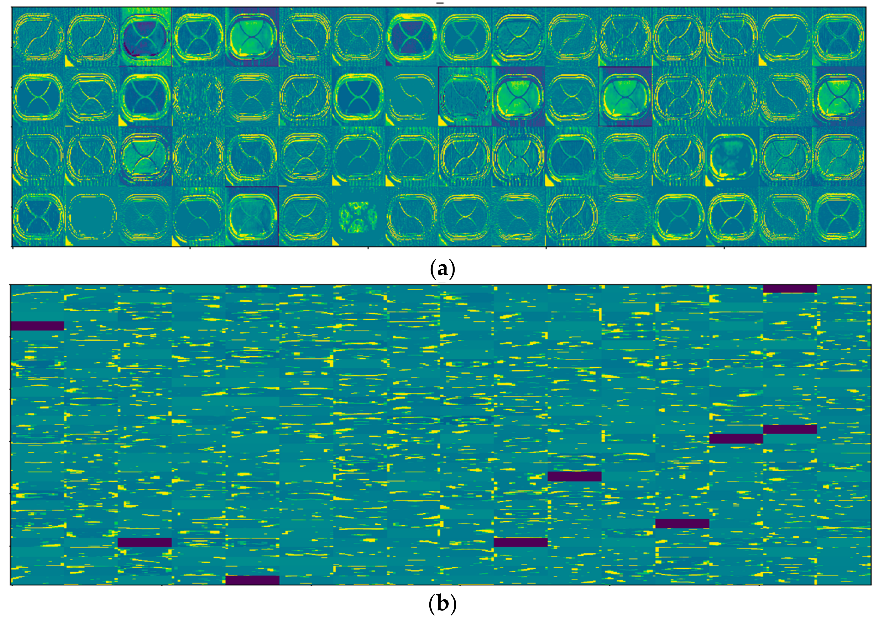
4.2. Visualizing What the CNNs Learned

To better observe this optimized model, we visualized the intermediate CNNs outputs (intermediate activations) for an input image. This helped us to better understand what the CNNs learned, and how to extract and present the learning representations in a human-readable form [32].

As shown in Figure 6, two layers were chosen to show these visualized feature maps, and the content of every channel was plotted as a 2D image independently. The first convolutional layer (Figure 6a), with 64 channels, showed each part of the welding area clearly. Like a collection of various edge detectors, the activations retained almost all the details present in the initial image. The ninth convolutional layer (Figure 6b) had 512 channels, and the image was no longer recognizable and some channels were black. As the depth of the layers increased, the activations became increasingly abstract and less visually interpretable. Higher presentations carried increasingly less information about the visual content of the image, and increasingly more information related to the class of the image. The sparsity of the activations increased with the depth of the layer. Specifically, in the first layer, all filters were activated by the input image, whereas in subsequent layers, some filters were black. This means that the pattern encoded by the filter was not found in the input image.

5. Conclusions

In conclusion, focusing on the requirement of laser welding quality inspection, we proposed an optimized CNN model to achieve the defect classification of the surface welding area of a safety vent based on a VGG-16 conv_base, which was trained on a large database. As a comparison, we classified the welding area images using five CNNs (AlexNet, VGG-16, Resnet-50, Densenet-121, and MobileNetV3-Large) to carry out three-classifications and two-classifications, respectively. Amongst these models, Resnet-50 and MobileNetV3-Large are the state-of-the-art deep learning algorithms, which are faster than other networks and exhibit very less training time. In the three-classifications task, comparatively, Resnet-50 behaved best and achieved the test dataset accuracy of 89.1%. Our optimized model (Pre-VGG-16) followed, whereas AlexNet, VGG-16, and MobileNetV3-Large behaved normal. In the Q-D two-classifications task, all of the CNNs models worked well. However, compared to our optimized model, these contrasting CNNs had the same problem of a long training and testing time, and thus led to lower efficiency. This increases industrial costs when the efficiency of the training dataset and testing dataset are not sufficiently high. Then, we modified the VGG model based on the theory of transfer learning and adopted a pre-training method to train the model. Using this optimized model, we achieved state-of-the-art performance for an application of the welding area defect classification, that is, the test accuracy was as high as 99.87% using over 8000 training images on an industrial computer. Additionally, the model had a lower fault positive rate of 0.16%, and it trained and predicted images quickly on an industrial computer. Moreover, the optimized model was not susceptible to the illumination environment and image size. It essentially meets the high accuracy requirement of industrial inspection. Furthermore, the convolution layer and classification results were visualized well, which can help operators to easily observe and adjust the model flexibly. To summarize, the experimental results prove that the improved VGG-16 model is superior to several contrasting CNNs and could provide a reference for designing relevant defect classification tasks using deep learning.

References

1. Lee, S.S.; Kim, T.H.; Hu, S.J.; Cai, W.W.; Abell, J.A. Joining Technologies for Automotive Lithium-Ion Battery Manufacturing: A Review. In Proceedings of the ASME 2010, International Manufacturing Science and Engineering Conference, Erie, PA, USA, 12–15 October 2010; pp. 541–549. [Google Scholar]
2. Shawn Lee, S.; Hyung Kim, T.; Jack Hu, S.; Cai, W.W.; Abell, J.A.; Li, J. Characterization of Joint Quality in Ultrasonic Welding of Battery Tabs. J. Manuf. Sci. Eng. 2013, 135, 021004. [Google Scholar] [CrossRef]
3. Muhammad, J.; Altun, H.; Abo-Serie, E. A robust butt welding seam finding technique for intelligent robotic welding system using active laser vision. Int. J. Adv. Manuf. Technol. 2018, 94, 13–29. [Google Scholar] [CrossRef]
4. Thornton, M.; Han, L.; Shergold, M. Progress in NDT of resistance spot welding of aluminium using ultrasonic C-scan. NDT E Int. 2012, 48, 30–38. [Google Scholar] [CrossRef]
5. Lashkia, V. Defect detection in X-ray images using fuzzy reasoning. Image Vision Comput. 2001, 19, 261–269. [Google Scholar] [CrossRef]
6. Jiaxin, S.; Han, S.; Dong, D.; Li, W.; Huayong, C. Automatic weld defect detection in real-time X-ray images based on support vector machine. In Proceedings of the 4th International Congress on Image and Signal Processing (CISP 2011), Shanghai, China, 15–17 October 2011; pp. 1842–1846. [Google Scholar]
7. Wu, H.; Zhang, X.; Xie, H.; Kuang, Y.; Ouyang, G. Classification of Solder Joint Using Feature Selection Based on Bayes and Support Vector Machine. IEEE Trans. Compon. Pack. Manuf. Technol. 2013, 3, 516–522. [Google Scholar] [CrossRef]
8. Fonseka, C.; Jayasinghe, J. Implementation of an Automatic Optical Inspection System for Solder Quality Classification of THT Solder Joints. IEEE Trans. Compon. Pack. Manuf. Technol. 2019, 9, 353–366. [Google Scholar] [CrossRef]
9. Besl, P.; Delp, E.; Jain, R. Automatic visual solder joint inspection. IEEE J. Robot. Autom. 1985, 1, 42–56. [Google Scholar] [CrossRef]
10. Cai, N.; Lin, J.; Ye, Q.; Wang, H.; Weng, S.; Ling, B.W. A New IC Solder Joint Inspection Method for an Automatic Optical Inspection System Based on an Improved Visual Background Extraction Algorithm. IEEE Trans. Compon. Packag. Manuf. Technol. 2016, 6, 161–172. [Google Scholar]
11. Jiang, J.; Cheng, J.; Tao, D. Color Biological Features-Based Solder Paste Defects Detection and Classification on Printed Circuit Boards. IEEE Transact. Compon. Packag. Manuf. Technol. 2012, 2, 1536–1544. [Google Scholar] [CrossRef]
12. Yang, Z.; Ye, Q.; Wang, H.; Liu, G.; Cai, N. IC solder joint inspection based on the Gaussian mixture model. Solder. Surf. Mount Technol. 2016, 28, 207–214. [Google Scholar]
13. Song, J.D.; Kim, Y.G.; Park, T.H. SMT defect classification by feature extraction region optimization and machine learning. Int. J. Adv. Manuf. Technol. 2019, 101, 1303–1313. [Google Scholar] [CrossRef]
14. Yun, T.S.; Sim, K.J.; Kim, H.J. Support vector machine-based inspection of solder joints using circular illumination. Electron. Lett. 2000, 36, 949–951. [Google Scholar] [CrossRef]
15. Hongwei, X.; Zhang, X.; Yongcong, K.; Gaofei, O. Solder Joint Inspection Method for Chip Component Using Improved AdaBoost and Decision Tree; IEEE: New Jersey, NJ, USA, 2011; Volume 1. [Google Scholar]
16. Song, J.-D.; Kim, Y.-G.; Park, T.-H. Defect Classification Method of PCB Solder Joint by Color Features and Region Segmentation. J. Instit. Control Robot. Syst. 2017, 23, 1086–1091. [Google Scholar] [CrossRef]
17. Lecun, Y.; Bengio, Y.; Hinton, G. Deep learning. Nature 2015, 521, 436–444. [Google Scholar] [CrossRef]
18. Krizhevsky, A.; Sutskever, I.; Hinton, G.E. ImageNet Classification with deep Convolutional Neural Networks, Proceedings of the 25th International Conference on Neural Information Processing Systems, Siem Reap, Cambodia, 13–16 December 2018—Volume 1; Curran Associates Inc.: Lake Tahoe, NV, USA, 2012; pp. 1097–1105. [Google Scholar]
19. Simonyan, K.; Zisserman, A. Very Deep Convolutional Networks for Large-Scale Image Recognition. arXiv 2014, arXiv:1409.1556. [Google Scholar]
20. Prasasti, A.L.; Mengko, R.K.W.; Adiprawita, W. Vein Tracking Using 880nm Near Infrared and CMOS Sensor with Maximum Curvature Points Segmentation, Proceedings of the 7th Wacbe World Congress on Bioengineering 2015, Singapore, 6–8 July 2015; Goh, J., Lim, C.T., Eds.; Springer: New York, NY, USA, 2015; Volume 52, pp. 206–209. [Google Scholar]
21. Chen, Y.-J.; Fan, C.-Y.; Chang, K.-H. Manufacturing intelligence for reducing false alarm of defect classification by integrating similarity matching approach in CMOS image sensor manufacturing. Comput. Indust. Eng. 2016, 99, 465–473. [Google Scholar] [CrossRef]
22. Qawaqneh, Z.; Abu Mallouh, A.; Barkana, B.D. Deep Convolutional Neural Network for Age Estimation based on VGG-Face Model. arXiv 2017, arXiv:1709.01664. [Google Scholar]
23. Donahue, J.; Jia, Y.; Vinyals, O.; Hoffman, J.; Zhang, N.; Tzeng, E.; Darrell, T. DeCAF: A Deep Convolutional Activation Feature for Generic Visual Recognition. arXiv 2013, arXiv:1310.1531. [Google Scholar]
24. Feng, L.; Po, L.-M.; Li, Y.; Xu, X.; Yuan, F.; Cheung, T.C.-H.; Cheung, K.-W. Integration of image quality and motion cues for face anti-spoofing: A neural network approach. J. Vis. Commun. Image Represent. 2016, 38, 451–460. [Google Scholar] [CrossRef]
25. Xu, B.; Wang, N.; Chen, T.; Li, M. Empirical Evaluation of Rectified Activations in Convolutional Network. arXiv 2015, arXiv:1505.00853. [Google Scholar]
26. Liu, W.; Wen, Y.; Yu, Z.; Yang, M. Large-Margin Softmax Loss for Convolutional Neural Networks. arXiv 2016, arXiv:1612.02295. [Google Scholar]
27. Wilson, A.C.; Roelofs, R.; Stern, M.; Srebro, N.; Recht, B. The Marginal Value of Adaptive Gradient Methods in Machine Learning; NIPS: San Diego, CA, USA, 2017; pp. 4148–4158. [Google Scholar]
28. Sermanet, P.; Eigen, D.; Zhang, X.; Mathieu, M.; Fergus, R.; LeCun, Y. OverFeat: Integrated Recognition, Localization and Detection using Convolutional Networks; Cornell University: Ithaca, NY, USA, 2013. [Google Scholar]
29. He, K.; Zhang, X.; Ren, S.; Sun, J. Deep Residual Learning for Image Recognition. arXiv 2015, arXiv:1512.03385. [Google Scholar]
30. Huang, G.; Liu, Z.; van der Maaten, L.; Weinberger, K.Q. Densely Connected Convolutional Networks; Cornell University: Ithaca, NY, USA, 2016. [Google Scholar]
31. Howard, A.; Sandler, M.; Chu, G.; Chen, L.-C.; Chen, B.; Tan, M.; Wang, W.; Zhu, Y.; Pang, R.; Vasudevan, V.; et al. Searching for MobileNetV3. arXiv 2019, arXiv:1905.02244. [Google Scholar]
32. Zeiler, M.D.; Fergus, R. Visualizing and Understanding Convolutional Networks; Springer International Publishing: Cham, Switzerland, 2014; pp. 818–833. [Google Scholar]
Figure 1. Welding area image acquisition setup.
Applsci 10 00933 g001
Figure 2. Three different types of welding area images: (a) Normal, (b) Porosity, and (c) Level Misalignment.
Applsci 10 00933 g002aApplsci 10 00933 g002b
Figure 3. Modification of the Visual Geometry Group (VGG)-16 model.
Applsci 10 00933 g003
Figure 4. Prediction score result for a test image.
Applsci 10 00933 g004
Figure 5. Experimental results of the welding area defect dataset: (a) training and validation accuracy; (b) training and validation loss.
Applsci 10 00933 g005
Figure 6. Visualization of the intermediate activations: (a) the first convolutional layer in the CNNs, (b) the ninth convolutional layer in the CNNs.
Applsci 10 00933 g006