Non-Poissonian Earthquake Occurrence Probability through Empirical Survival Functions

School of Civil Engineering, University of Basilicata, I-85100 Potenza, Basilicata, Italy
Appl. Sci. 2020, 10(3), 838; https://doi.org/10.3390/app10030838
Submission received: 13 December 2019
/
Revised: 15 January 2020
/
Accepted: 18 January 2020
/
Published: 24 January 2020
(This article belongs to the Special Issue Evaluation and Mitigation of Seismic Risk for Existing Buildings, Structures, and Infrastructures)
Abstract
:Earthquake engineering normally describes earthquake activity as a Poissonian process. This approximation is simple, but not entirely satisfactory. In this paper, a method for evaluating the non-Poissonian occurrence probability of seismic events, through empirical survival probability functions, is proposed. This method takes into account the previous history of the system. It seems robust enough to be applied to scant datasets, such as the Italian historical earthquake catalog, comprising 64 events with M ≥ 6.00 since 1600. The requirements to apply this method are (1) an acceptable knowledge of the event rate, and (2) the timing of the last two events with magnitude above the required threshold. I also show that it is necessary to consider all the events available, which means that de-clustering is not acceptable. Whenever applied, the method yields a time-varying probability of occurrence in the area of interest. Real cases in Italy show that large events obviously tend to occur in periods of higher probability.
1. Introduction
Seismology is a discipline in which there are few certainties. The main one is that earthquakes are self-similar over an incredibly wide scale since, for large sets of events, the Gutenberg–Richter relationship [1] is always valid. Due to the complexity of the phenomenon, every practical application is based on the assumption that the occurrence of earthquakes can be approximated as a Poissonian behavior. In particular, Reference [2] represents the basis of most of modern applications, as it is simple and requires only knowledge of the event occurrence rate in the area of interest.
However, worldwide seismic activity does not follow a Poisson distribution [3], not even locally [4]. Furthermore, as the underlying physical processes are not yet properly understood, the existing non-Poissonian statistical models, which were proposed by several authors [5,6,7,8,9,10], are not really satisfactory.
Another problem is that methods such as that in Reference [2] require the de-clustering of earthquake datasets; however, (1) de-clustering is always a subjective procedure, and (2) it is plainly wrong, as it is impossible to distinguish between main events, aftershocks, and the background seismicity [11].
I propose a completely different approach, based on empirical survival probability functions, which extends, in practice, the approach proposed in Reference [3]. In such a way, it is possible to retrieve a time-varying probability for the occurrence of the next event of interest.
The motivation for this paper lies in the fact that previous studies on non-Poissonian earthquake behavior focused on finding a way to analytically describe the true distribution; however, nobody really attempted to put it to full use for hazard purposes. As it will likely be impossible to find a universal analytical description until we understand the underlying processes that cause earthquakes, I resolved to propose a new approach.
2. Data
I used three different earthquake catalogs. The first was the ISC-GEM catalog ver 6.0 [12,13,14]; the second was that produced by the Southern California Earthquake Center [15]; the third was the Italian CPTI15 [16], with numerous additions that I illustrate in detail.
The ISC-GEM catalog is a worldwide instrumental catalog, spanning from 1904 to 2015. The main set I selected (DS1) considers magnitude M ≥ 6.00 and depth D ≤ 60 km. The time interval goes from 1950 to 2015, as 1950 seemed to represent a turning point in the completeness of the catalog such that, for the purposes of this paper, the set could be considered to be complete. A few tens of events, however, had to be discarded, as many large events were, in fact, multiple events; global catalogs often fail to detect these, and the completeness in such cases is almost null. An example I am personally aware of [17] is the 1980 Irpinia earthquake, which was a multiple event composed of three different M > 6 earthquakes which took place, spaced about 20 s one from the other, along different faults located a few tens of kilometers from each other. The global catalogs, including the ISC-GEM one, consider this earthquake to be a single event. However, there are some cases when the multiple events in ISC-GEM are reported separately. Consequently, I eliminated the second earthquake from the dataset, whenever two events were spaced less than twice the sum of the length of their faults (computed according to Reference [18]) and had a time interval consistent with a rupture propagation speed of at least 500 m/s. After this operation, 6921 events remained. There was another reason. Most of the solutions, in terms of magnitude, in the ISC-GEM were from the GCMT catalog [19,20]; the latter does not distinguish between two proximal events, being a spectral method, and includes the sum (in terms of moment) of both events.
The second dataset (DS2) also originated from the ISC-GEM catalog, and it is composed of events with magnitude M ≥ 8.50 and depth D ≤ 60 km. The time interval goes from 1918 to 2015. There are 16 events in it.
The third dataset (DS3) is the de-clustered version of DS2, which is made up by 14 events.
The fourth dataset (DS4) is composed of all the earthquakes reported by the Southern California Earthquake Center with magnitude M ≥ 3.00 between 1980 and 2018. It is made up of 11,852 events. I chose this magnitude threshold for two reasons; it ensures completeness also in the most peripheral areas—particularly offshore—and it does the same for the aftermath of the largest events.
The fifth dataset (DS5) is composed by 64 events which caused noticeable damage in Italian territories from 1600 to 2016. They yield magnitude M ≥ 6.00 and depth D presumably ≤45 km. Of these events, 61 are from the CPTI15, which ends in 2014, while the last three (all occurring in 2016) are from the GCMT catalog. One event, the 1743 Ionian Sea, was excluded, even though it caused heavy damage in southern Puglia, since its epicentral location was very far offshore [21] and, at that distance, only very large events could be detected; the seismic record in that area, therefore, is surely not complete.
DS5 was a validated set, but it did not pass even a simple completeness Gutenberg–Richter test. I devised a way to complete it, from a statistical viewpoint, which formed the sixth and last dataset (DS6) (see File S1 in supplementary). The rationale is that the vast majority of the missing events were already reported in the catalog; however, for some reason, their magnitude was underestimated. Obviously, it could also occur that events with M ≥ 6.00 were overestimated. I believed, however, that the true solution was hidden in this dataset. In particular, I split the 27 March 1638 event into two events, according to Reference [22]. Then, I chose all the events reported in the CPTI15 catalog that may have represented underestimated events. In doing so, I obviously introduced a high degree of subjectivity; however, I followed some rules based on the similarity of macroseismic effects, with respect to modern earthquakes, where good Mw estimates are available. Therefore, events that took place in the Northern Plains may have been underestimated by as much as 0.6–0.7, in terms of magnitude, as observed during the 2012 seismic sequence. Scant macroseismic fields with some high-intensity points could provide an indication that a larger event was badly recorded, particularly in the 17th and 18th centuries. Conversely, a more recent event with high intensities in few locations and several lower-intensity observations all grouped within a short distance is an indication of a lower-magnitude event. A highly varied distribution of damage level over a wider area is an indication of deeper events that could be discarded; however, this is not true in the Northern Plains and Southern Apennines, where there was relevant activity at depths of over 20 km. In the pre-instrumental era, I selected, on the basis of this approach, a certain number of events and, in some cases, I re-modulated the standard deviation, σ, in order to allow it to encompass (within 2σ) the M = 6.0 threshold. As far as instrumental era events are concerned, I subdivided them into two periods, pre- and post-1976. Events before 1976 have the magnitude computed as a weighted average [23] between the macroseismic and the instrumental magnitude, where I selected the ISC-GEM value as the instrumental magnitude. In one case (17 May 1916), I also averaged over a third solution [24]. From 1976 onward, I exclusively used CMT magnitude estimates. In particular, before 2004, I took the average of the GCMT and RCMT [25,26] magnitude estimates, where both were available. Since 2004, GCMT extended its analysis to the S-waves, a feature that was typical of RCMT. This means that the two solutions are strongly correlated; therefore, I limited use to the GCMT solutions only from 2004. In the instrumental era, I also sometimes modified σ, such as to give a certain degree of freedom to cross, in both directions, the M = 6.0 threshold. The dataset DS6 comprises 135 events and can be downloaded at www.seisrisk.org.
The final consideration, for both DS5 and DS6, is that I rounded the timing to the nearest minute. Sometimes minutes, hours, and even, in a few cases, the day of month were missing; in such cases, I always used the central value of the undefined field/fields.
3. Method: Empirical Approach
The most common approach to describing the earthquake occurrence probability is through the survival probability function, that is, the probability that an inter-event time interval will be greater than a given value . This is tantamount to evaluating . In the case of a Poissonian distribution, we have
where is the mean. This means that we can normalize, by simply dividing each by .
When we have a set of real data with , the observed SP is simply
which can also be normalized.
The first to propose the usage of real data, instead of trying to model them, was Reference [3], as stated above. I simply extend his approach.
There is a further step I introduce before looking at the real data. Even if we do not know what the survival probability function is—and we will likely never be able to model it simply—we can evaluate how far it departs from a Poissonian distribution through a transformation. This means that we can express it as
and, then, define as
We may immediately evaluate this function if it can be approximated by a Poissonian decay in any interval, as, in that case, it will yield a flattish trend.
I believe, moreover, that this approach is the optimal way of evaluating a survival probability function, as we know that it will decrease from one to zero asymptotically as increases and that this trend is anyway similar to that of , even though it is not exactly equal to it.
The last observation point with this method remains undefined, however, as it always yields .
A further clarification is that I avoided any consideration relative to data uncertainties, as this would distract us from examining the data trends. It is clear, however, that, as increases, the uncertainties become very large.
In Figure 1, both the normalized survival probability (left) and the normalized (right) are shown for DS1–DS4. A dashed line indicates the corresponding . It is evident that all the survival functions do not resemble a Poissonian decay, even the de-clustered M ≥ 8.50 one. In this case, if we focus on , we observe that it is actually (quite notably) increasing, as the graph is in logarithmic scale along both axes. However, the de-clustered pattern is totally different from that of those that were not de-clustered. As stated before, Reference [11] showed that it is impossible to distinguish between the background seismicity, main events, and aftershocks. I go a step further, showing that the future event occurrence probability is strongly influenced by the history of the time series, and that clustered events actually lead to a totally different occurrence probability at a long temporal distance from the cluster.
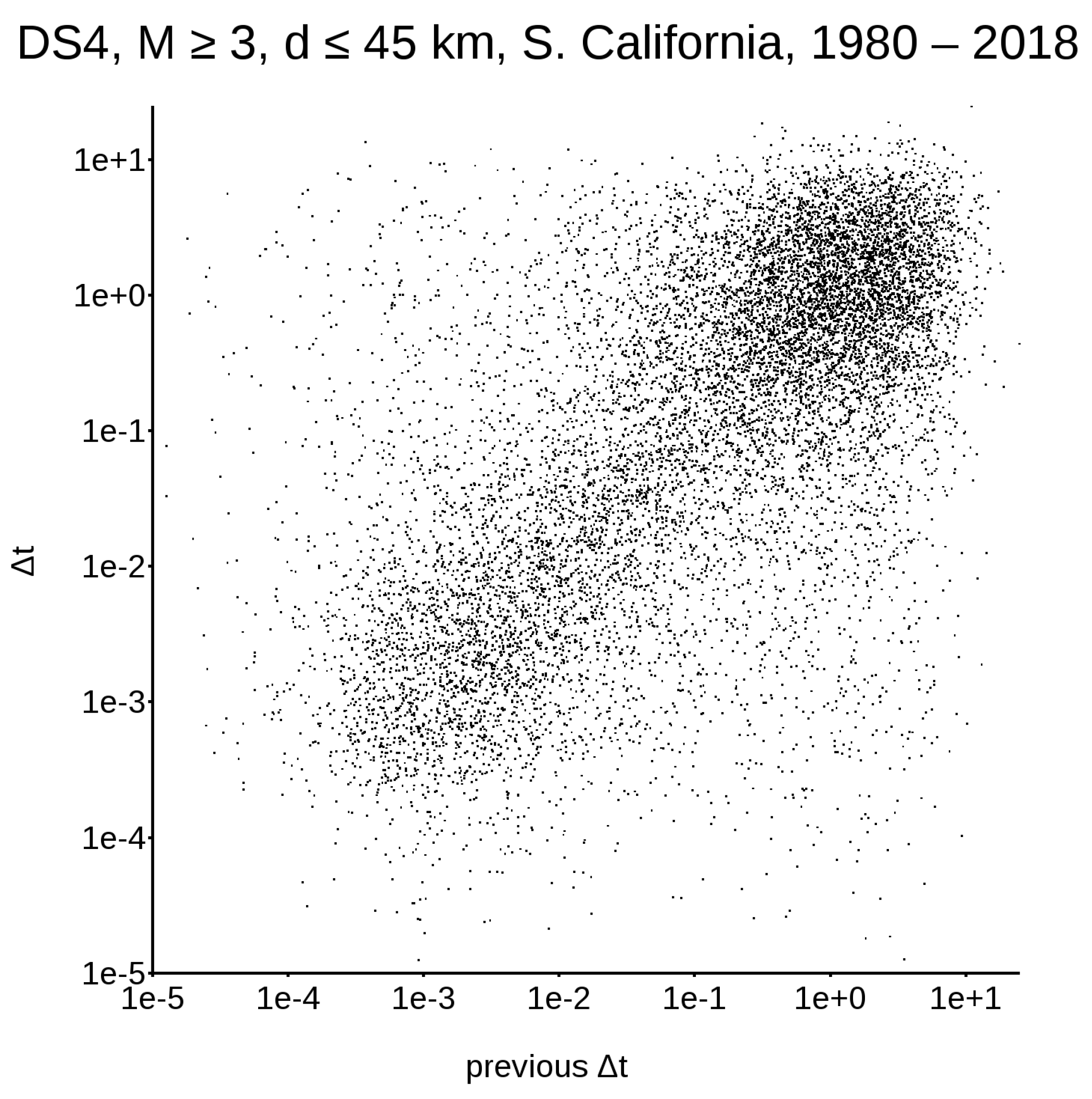
First of all, we need to consider that, if a dataset is non-Poissonian, it must have some memory in itself; this means that the classical representation, in terms of the survival probability function (as shown in Figure 1, left column), does not contain all the information required to describe the system’s evolution. To address this issue, let us concentrate on DS1 and DS4, the only very large datasets available. Figure 2 and Figure 3 show the distribution between earthquake triplets; in other words, for every plotted along the abscissa, is plotted along the ordinate. Figure 2, relative to the worldwide DS1, yields a single cluster in the upper right corner, while Figure 3, relative to the Californian DS4, yields two different clusters.
To understand how this distribution affects real data, I selected a narrow band along the abscissa (Figure 4) and recomputed both and using the normalized values from the whole dataset. The band width was chosen in such a way that there were at least 200 samples in each band (with the exclusion of the last one, to the right, where its number is barely above 50). A selection of some significant results is shown in Figure 5, relative to the worldwide dataset (DS1), and Figure 6 for the Californian dataset (DS4). A complete presentation of all the available SPs can be found in Appendix (see File S2 in supplementary).
To clarify what we can see up to now, we must go back to the event triplets. The narrow band refers to the time interval between the first and second events of the triplet, while the survival probability function is relative to the inter-event time interval between the second and the third events. We note that, disregarding the time interval between the first and second events, whenever the third event occurs over a short temporal interval, the survival probability distribution is very different from the Poissonian one, even though it is more non-Poissonian if the time interval between the first and second events is very small. This, however, could simply mean that events tend to cluster and, to evaluate the occurrence probability of events, we must firstly de-cluster. However, there is another remarkable feature; when the time interval between the first and second events is small, even when the third event occurs over a very large temporal interval (e.g., several times the dataset average), its occurrence probability is noticeably different from a Poissonian one. Conversely, if the time interval between the first and the second event is larger than the dataset average, the occurrence of the third event for large inter-event time intervals becomes almost Poissonian. This has two very interesting consequences. The first is that, whenever the previous events are clustered, their influence has an extremely long range. The second and maybe even more important consequence is that, given this long-range temporal influence, de-clustering is plainly wrong; this is true also for large-magnitude events.
The last feature which we must address is how to compute seismic hazard. By this, I mean, for instance, to evaluate the period of time that will yield a 10% occurrence probability. A simple answer would be that of Reference [3]. However, in a non-Poissonian approach, hazard would require continuous re-computation.
Let us consider an example (see Figure 7). Assume that that the of the second-to-last occurrence, with respect to the last event, is about 1.5. In this case, the appropriate survival probability function is represented by the solid line and, in that portion, the Poissonian probability would be represented by the dashed line. In this case, the two lines are almost indistinguishable. We can also suppose that no event occurred up to now, and that the time elapsed from the last event is . At this point, the future occurrence probability must still be one, such that the portion of the survival probability to the right of must be scaled in such a way that, at , the new survival probability function will be 1. In the example, this means multiplying it by about 3.02. The new function is represented by the dotted line. Therefore, if we want to estimate the time interval over which there will be a 10% probability of event occurrence, we need to use this new, scaled-up function. As a consequence, a correct assessment requires us first to build a survival probability function which takes into account the last inter-event time interval, and then to rescale this function, in order to take into account the elapsed time without events.
4. Discussion: Application to the Current Probability in Italy
An actual application is Italy. The historic Italian catalog CPTI15 is probably the best one in the world; unfortunately, being the best does not ensure that it is good enough. It is very rich, but not complete, dating back to about 1600. Thus, it is quite obvious that we cannot use it at face value. However, since earthquakes are self-similar, we can try to prove that the worldwide survival probability general function can be applied to the Italian events. On the basis of DS6, I created 106 datasets with randomly picked magnitudes, according to a Gaussian distribution, based on the catalog magnitudes and relative standard deviation. The obvious assumption was that all (or most) of the M ≥ 6 earthquakes are, in fact, contained in CPTI15, but that the magnitudes are either over- or under-estimated. The randomized datasets contained between 55 and 92 events each. I discretized each logarithmic decade into 20 bins, instead of directly using the observed . Then, I computed the survival probability function for each dataset, stacked it, and finally averaged it. As the event number was not constant, the most significant portion of the averaged survival probability function was where events tended to concentrate, that is, in the range between 0.1 and three.
In Figure 8, a comparison between DS1, DS5, and DS6 is shown, where the solid line is DS5, the dotted line is DS1, and the dashed line is DS6. We can observe that the similarity between DS1 and DS6, in the range of interest, is quite remarkable, even though it is also acceptable with respect to DS5. This means that, if we have a poor dataset, we can substitute it with a richer one with the same magnitude completeness, as long as we know precisely the timing of the last two events and have a realistic estimate of the event rate.
Evaluation of hazard is tricky from a computational viewpoint; that is, the application of what is shown in Figure 7 requires some further steps. First of all, we need to oversample the survival probability function which we will use (i.e., we need to discretize each logarithmic decade into at least 200 bins), and then we need to apply a smoothing technique, as the function would otherwise assume a step-like shape. I personally found that a Gaussian filter in the time domain with had an optimal response, since it ensures monotonic behavior (except for the very few initial points) and minimal differences with respect to the original function. However, I applied this filter not to the time domain function itself, but to its equivalent in the time logarithmic domain. As, in the very few initial points, it yielded a strong down-shoot followed by a very slight over-shoot, which brings the probability to over one; I included an initial logarithmic decade and padded it with ones. Finally, a specific generally requires interpolation between two samples, as it will follow the 90% threshold. I applied a simple linear interpolation technique, but more sophisticated approaches will yield a more refined result. The final step is to select the optimal bandwidth over which to compute the survival probability function. As my main reference dataset was DS1 (which has nearly 7000 events), I chose a band including the nearest 250 data points on both sides (500 total) of the specific value between the last and second-to-last events. In the case that this is either very small or very large and I do not have 250 events on both sides, I used the smallest or largest 500 , respectively.
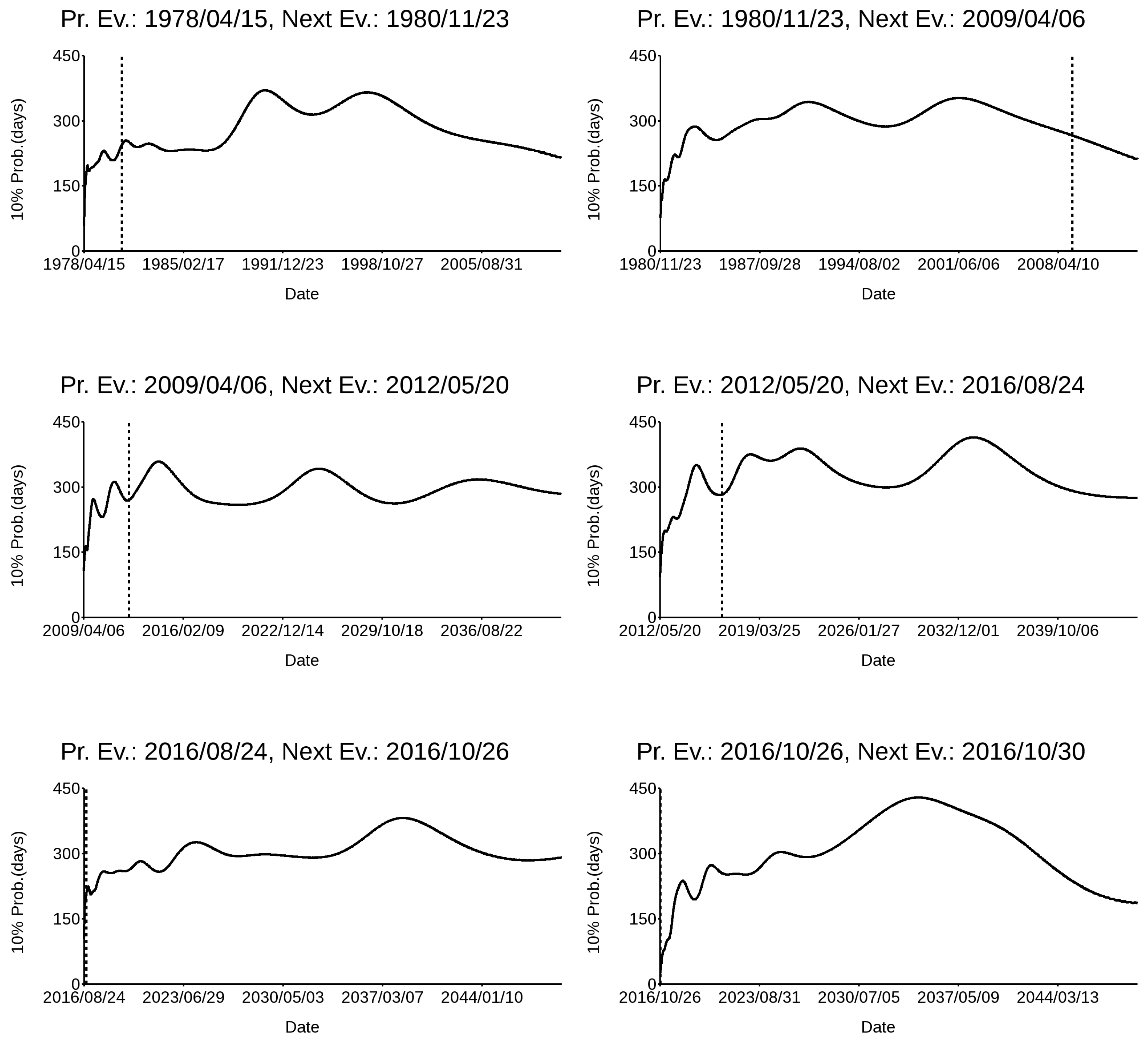
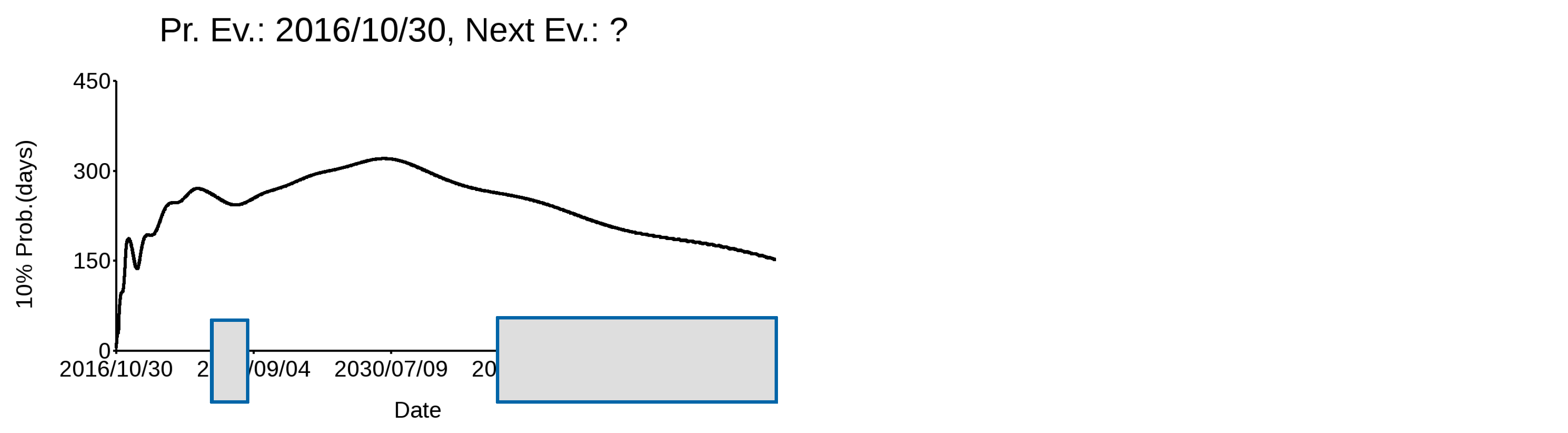
In Figure 9, the variation of the 10% probability time interval, expressed in days, with time after each of the last seven major earthquakes that hit the Italian territory since 1978 (Table 1) is shown. I limited this analysis to the last seven, since there were only eight major events with M ≥ 6.00 for which a CMT magnitude estimate was available, and the method I propose requires at least two events to estimate the occurrence probability of the next one. The event rate is calculated for each event on the basis of DS5—the validated CPTI15 dataset—excluding the more recent, yet to occur, events. The occurrence timing of the next event is shown with a dashed vertical line. It is noteworthy that the events all occur during graph minima, which actually correspond to increased probability time intervals. This means that, according to this pattern, the next event will likely occur either in the next few months, during spring–fall 2022, or after 2035, the latter two being highlighted by gray areas. It is obvious that we are simply discussing probabilities and that events can occur even with a highly improbable timing; nevertheless, we have an indication.
There is a final remark. The approach I propose works well for the Italian territory, as its b value is probably very similar to the world one. It should work for all those areas with similar characteristics. However, it could probably also be applied in areas where it is rather different, as the majority of events are anyway earthquakes whose magnitudes are nearer to the lower cut-off thresholds and, in this case, any change of the Gutenberg–Richter slope should not be too dramatic.
5. Conclusions
The method proposed in this paper takes into account, through empirical survival probability functions, the correlation between various events. It is evident that, if the probability of one event depends not only on the previous one but the previous two, the whole process can be back-traced indefinitely. This is tantamount to claiming that the events are all linked together, to some degree.
Another outcome is that de-clustering is plainly wrong, as the future evolution of the system strongly depends on clustered events, as well as the long-term temporal scale.
In terms of application, the method is still at an initial stage, but seems to be robust enough to be applicable to scant datasets, such as the Italian one, as long as we can estimate the event rate and we know, with precision, which were the last two events (above the considered magnitude threshold) that occurred in the area of interest. It is quite clear that, right now, it could have only civil protection purposes, but I do hope that it will be soon possible to extend it to building codes with minimal effort.
Supplementary Materials
The following are available online at https://www.mdpi.com/2076-3417/10/3/838/s1, File S1: Possible M6 in Italy since1600.xlsx and File S2: Appendix.pdf.
Funding
This research received no external funding.
Acknowledgments
The author thanks Marco Vona for continuous discussion about the topic of work and the encouragement to write this article. G. De Natale and an anonymous referee helped with useful suggestions.
Conflicts of Interest
The author declares no conflict of interest.
References
- Gutenberg, B.; Richter, C.F. Frequency of earthquakes in California. Bull. Seismol. Soc. Am. 1944, 34, 185–188. [Google Scholar]
- Cornell, C.A. Engineering Seismic Risk Analysis. Bull. Seismol. Soc. Am. 1968, 58, 1583–1606. [Google Scholar]
- Corral, A. Time-Decreasing Hazard and Increasing Time until the Next Earthquake. Phys. Rev. E 2005, 71, 017101. [Google Scholar] [CrossRef] [PubMed] [Green Version]
- Vecchio, A.; Carbone, V.; Sorriso-Valvo, L.; De Rose, C.; Guerra, I.; Harabaglia, P. Statistical properties of earthquakes clustering. Nonlin. Process. Geophys. 2008, 15, 333–338. [Google Scholar] [CrossRef]
- Corral, A. Universal local versus unified global scaling laws in the statistics of seismicity. Phys. A Stat. Mech. Appl. 2004, 340, 590–597. [Google Scholar] [CrossRef] [Green Version]
- Carbone, V.; Sorriso-Valvo, L.; Harabaglia, P.; Guerra, I. Unified scaling law for waiting times between seismic events. Europhys. Lett. 2005, 71, 1036. [Google Scholar] [CrossRef]
- Hasumi, T.; Akimoto, T.; Aizawa, Y. The Weibull-log Weibull distribution for interoccurrence times of earthquakes. Phys. A Stat. Mech. Appl. 2009, 388, 491–498. [Google Scholar] [CrossRef] [Green Version]
- Hasumi, T.; Chen, C.; Akimoto, T.; Aizawa, Y. The Weibull–log Weibull transition of interoccurrence time for synthetic and natural earthquakes. Tectonophysics 2010, 485, 9–16. [Google Scholar] [CrossRef]
- Michas, G.; Vallianatos, F.; Sammonds, P. Non-extensivity and long-range correlations in the earthquake activity at the West Corinth rift (Greece). Nonlin. Process. Geophys. 2013, 20, 713. [Google Scholar] [CrossRef] [Green Version]
- Michas, G.; Vallianatos, F. Stochastic modeling of nonstationary earthquake time series with long-term clustering effects. Phys. Rev. E 2018, 98, 042107. [Google Scholar] [CrossRef]
- Bak, P.; Christensen, K.; Danon, L.; Scanlon, T. Unified scaling law for earthquakes. Phys. Rev. Lett. 2002, 88, 178501. [Google Scholar] [CrossRef] [PubMed] [Green Version]
- Storchak, D.A.; Di Giacomo, D.; Bondár, I.; Engdahl, E.R.; Harris, J.; Lee, W.H.K.; Villaseñor, A.; Bormann, P. Public Release of the ISC-GEM Global Instrumental Earthquake Catalogue (1900–2009). Seismol. Res. Lett. 2013, 84, 810–815. [Google Scholar] [CrossRef] [Green Version]
- Storchak, D.A.; Di Giacomo, D.; Engdahl, E.R.; Harris, J.; Bondár, I.; Lee, W.H.K.; Bormann, P.; Villaseñor, A. The ISC-GEM Global Instrumental Earthquake Catalogue (1900–2009): Introduction. Phys. Earth Planet. Int. 2015, 239, 48–63. [Google Scholar] [CrossRef]
- Di Giacomo, D.; Engdahl, E.R.; Storchak, D.A. The ISC-GEM Earthquake Catalogue (1904–2014): Status after the Extension Project. Earth Syst. Sci. Data 2018, 10, 1877–1899. [Google Scholar] [CrossRef] [Green Version]
- SCEDC. Southern California Earthquake Center. Caltech. Dataset 2013. [Google Scholar] [CrossRef]
- Rovida, A.; Locati, M.; Camassi, R.; Lolli, B.; Gasperini, P. (Eds.) Catalogo Parametrico dei Terremoti Italiani (CPTI15); Istituto Nazionale di Geofisica e Vulcanologia (INGV): Rome, Italy, 2016. [Google Scholar] [CrossRef]
- Vaccari, F.; Harabaglia, P.; Suhadolc, P.; Panza, G.F. The Irpinia (Italy) 1980 earthquake: Waveform modelling of accelerometric data and macroseismic considerations. Ann. Geophys. 1993, 36, 93–108. [Google Scholar] [CrossRef]
- Wells, D.; Coppersmith, K. New Empirical Relationships among Magnitude, Rupture Length, Rupture Width, Rupture Area, and Surface Displacement. Bull. Seismol. Soc. Am. 1994, 84, 974–1002. [Google Scholar]
- Dziewonski, A.M.; Chou, T.-A.; Woodhouse, J.H. Determination of earthquake source parameters from waveform data for studies of global and regional seismicity. J. Geophys. Res. 1981, 86, 2825–2852. [Google Scholar] [CrossRef]
- Ekström, G.; Nettles, M.; Dziewonski, A.M. The global CMT project 2004–2010: Centroid-moment tensors for 13,017 earthquakes. Phys. Earth Planet. Inter. 2012, 200–201, 1–9. [Google Scholar] [CrossRef]
- Nappi, R.; Gaudiosi, G.; Alessio, G.; De Lucia, M.; Porfido, S. The environmental effects of the 1743 Salento earthquake (Apulia, southern Italy): A contribution to seismic hazard assessment of the Salento Peninsula. Nat. Hazards 2017, 86, S295–S324. [Google Scholar] [CrossRef] [Green Version]
- Galli, P.; Bosi, V. Catastrophic 1638 earthquakes in Calabria (southern Italy): New insights from paleoseismological investigation. J. Geophys. Res. 2004, 108. [Google Scholar] [CrossRef] [Green Version]
- Gasperini, P.; Lolli, B.; Vannucci, G. Empirical Calibration of Local Magnitude Data Sets Versus Moment Magnitude in Italy. Bull. Seismol. Soc. Am. 2013, 103, 2227–2246. [Google Scholar] [CrossRef]
- Caciagli, M.; Batlló, J. The Rimini earthquake of 17th May 1916 (Italy): From historical data to seismic parameters. In Proceedings of the European Seismological Commission ESC 2008, 31st General Assembly, Crete, Greece, 7–12 September 2008; p. 113. [Google Scholar]
- Pondrelli, S. European-Mediterranean Regional Centroid-Moment Tensors Catalog (RCMT); Istituto Nazionale di Geofisica e Vulcanologia (INGV): Rome, Italy, 2002. [Google Scholar] [CrossRef]
- Pondrelli, S.; Ekström, G.; Morelli, A. Seismotectonic re-evaluation of the 1976 Friuli, Italy, seismic sequence. J. Seismol. 2001, 5, 73–83. [Google Scholar] [CrossRef]
Figure 1.
Survival probability (left) and (right) for datasets 1–4 (DS1–DS4). Solid lines refer to empirical functions, while dashed lines refer to Poissonian ones.
Figure 1.
Survival probability (left) and (right) for datasets 1–4 (DS1–DS4). Solid lines refer to empirical functions, while dashed lines refer to Poissonian ones.
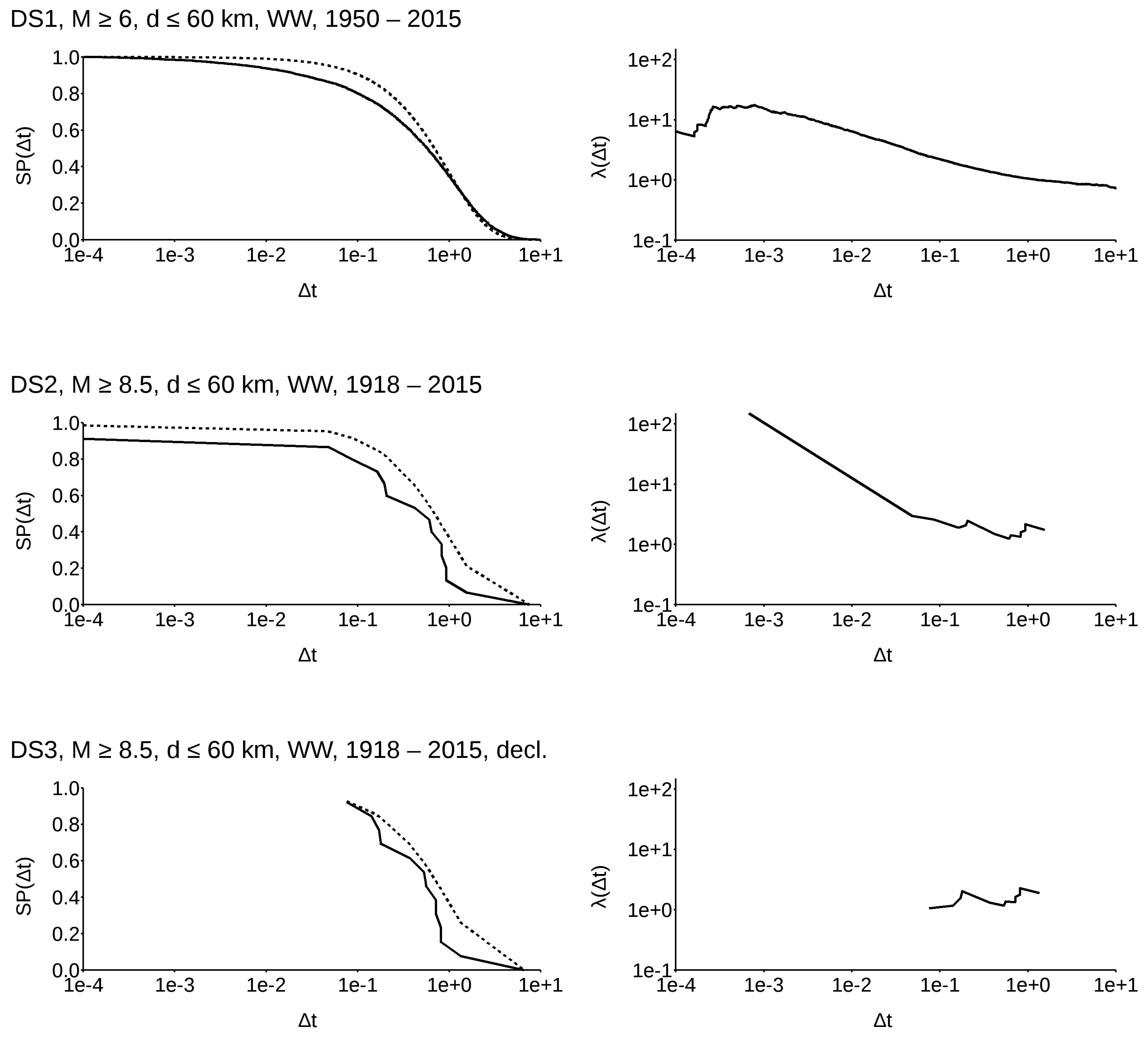
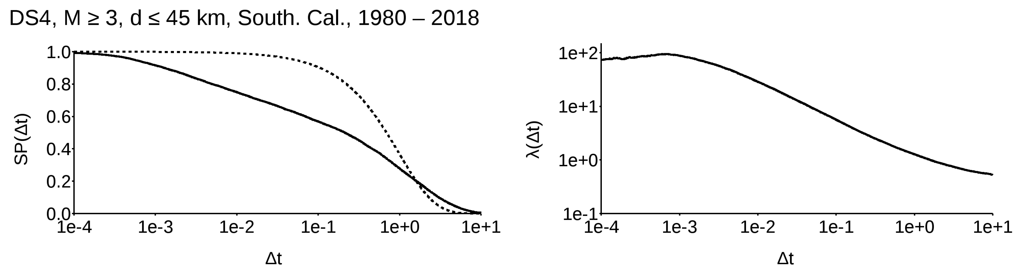
Figure 2.
Distribution between earthquake triplets in DS1; abscissa: , ordinate: .
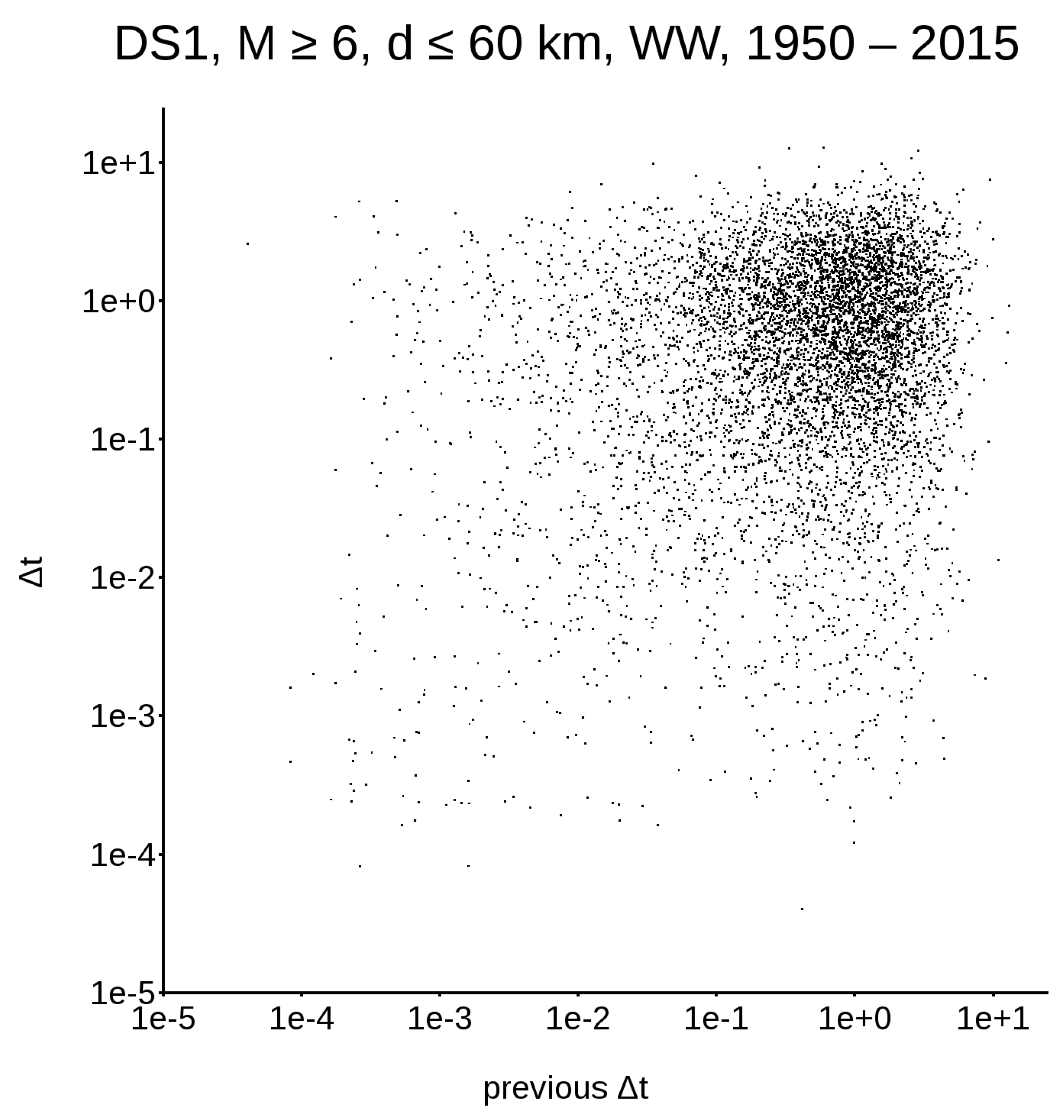
Figure 3.
Distribution between earthquake triplets in DS4; abscissa: , ordinate: .

Figure 4.
Example of how events are selected to compute the new survival probability functions depending on the previous .
Figure 4.
Example of how events are selected to compute the new survival probability functions depending on the previous .
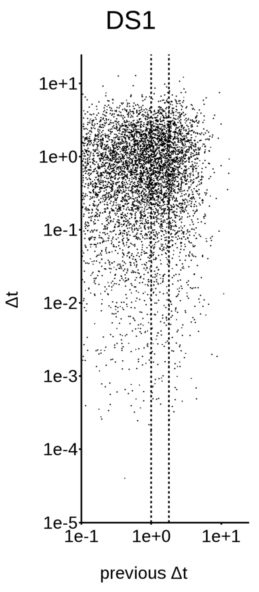
Figure 5.
Survival probability (left) and (right) for DS1 along the narrow bands, selected as in Figure 4. Solid lines refer to empirical functions, while dashed lines refer to Poissonian ones.
Figure 5.
Survival probability (left) and (right) for DS1 along the narrow bands, selected as in Figure 4. Solid lines refer to empirical functions, while dashed lines refer to Poissonian ones.
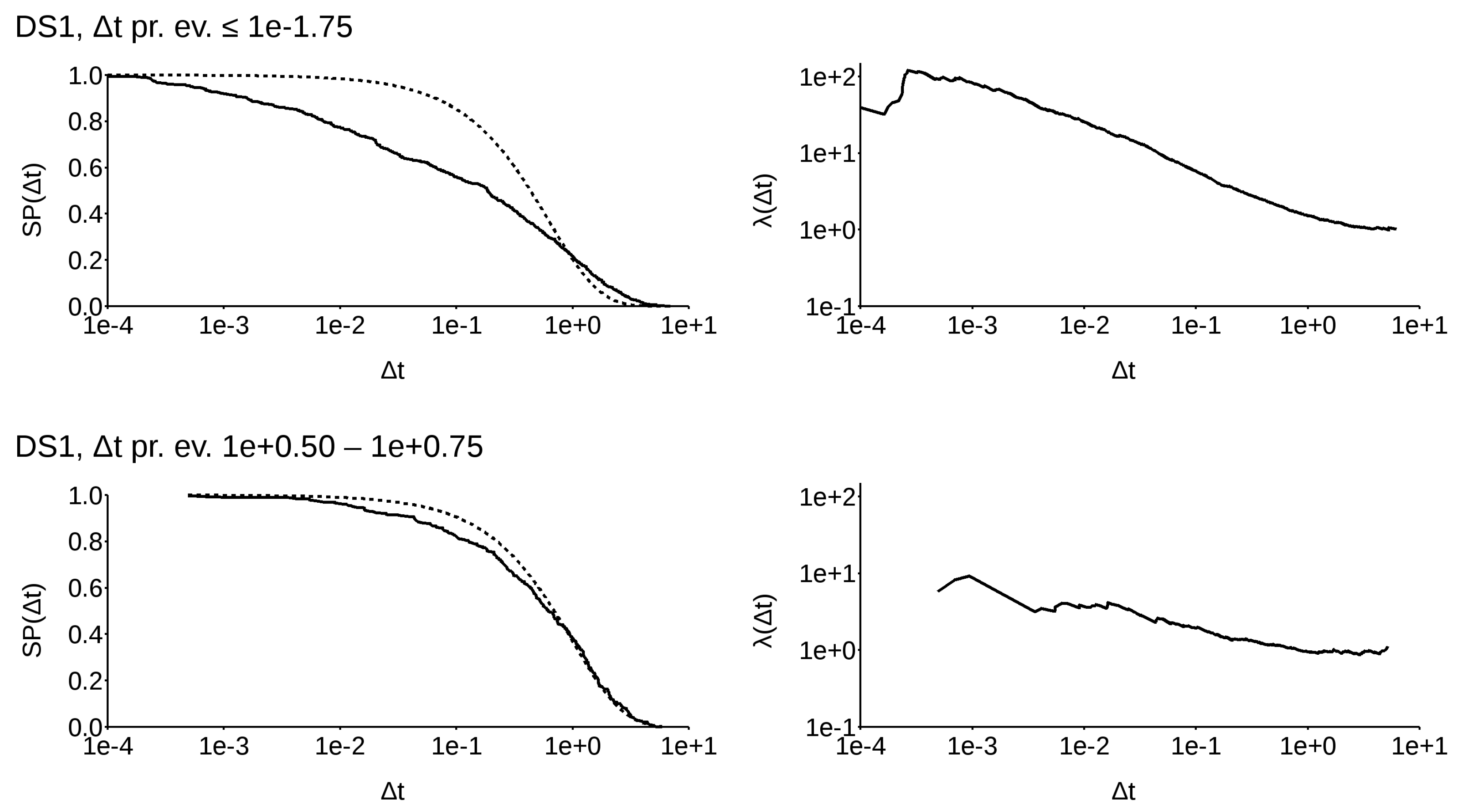
Figure 6.
Survival probability (left) and (right) for DS4 along the narrow bands, selected as in Figure 4. Solid lines refer to empirical functions, while dashed lines refer to Poissonian ones.
Figure 6.
Survival probability (left) and (right) for DS4 along the narrow bands, selected as in Figure 4. Solid lines refer to empirical functions, while dashed lines refer to Poissonian ones.
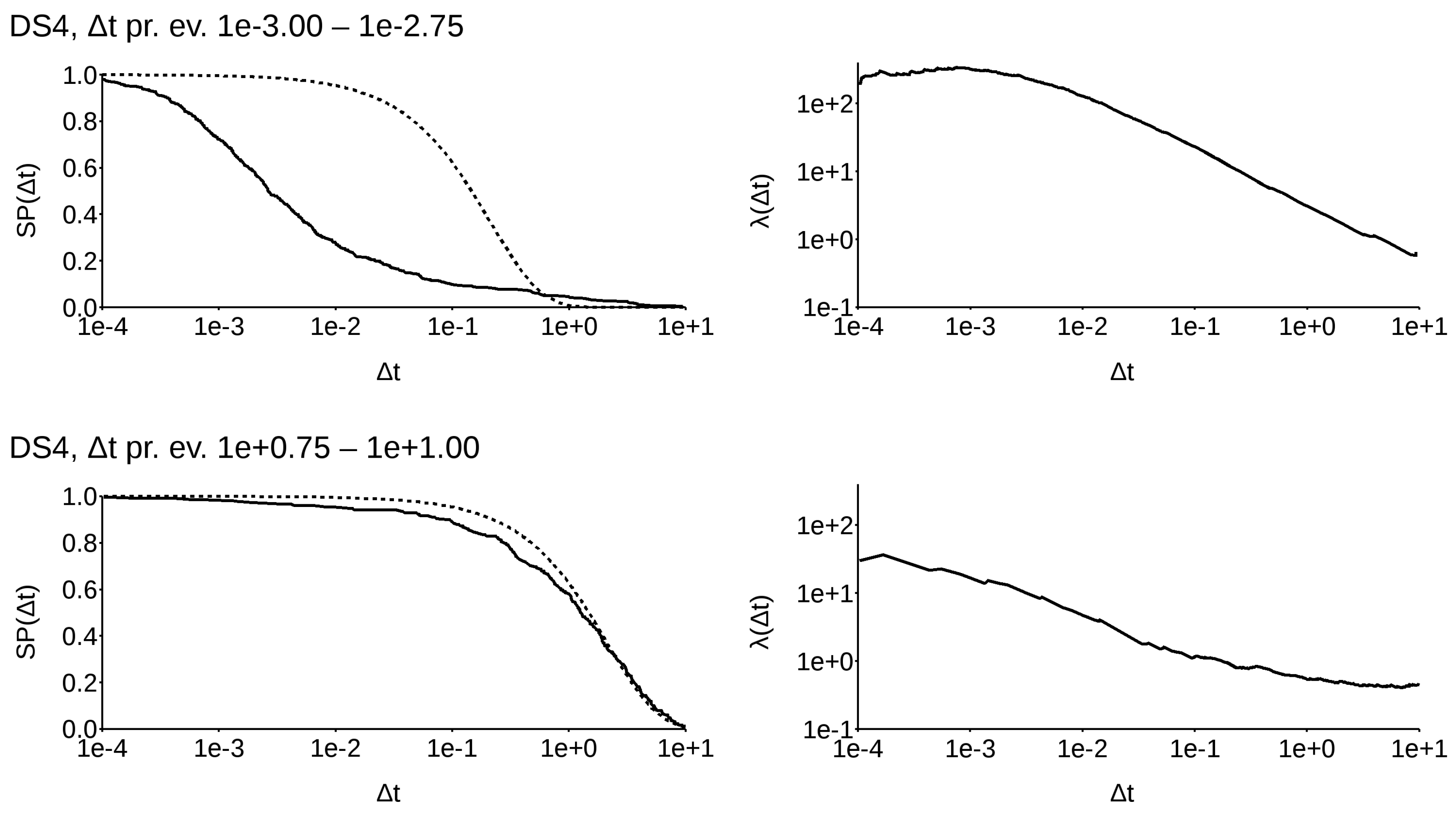
Figure 7.
Method of computation of the 10% probability time interval at the elapsed time , given a specific between the last and the second-to-last event. The solid line refers to the empirical function, the dashed line refers to the Poissonian one, and the dotted line refers to the new, rescaled empirical one.
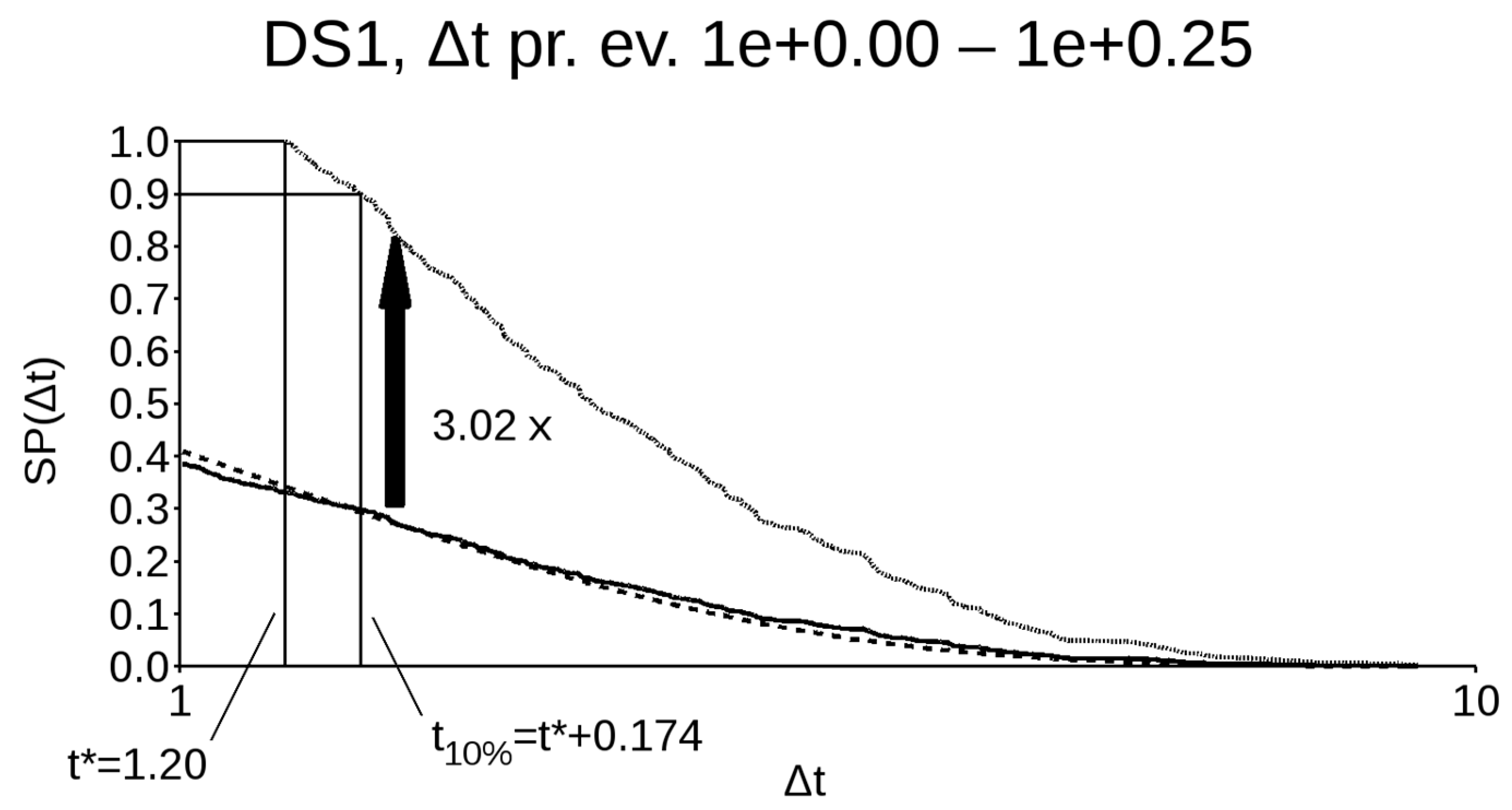
Figure 8.
Survival probability relative to DS1, DS5, and DS6. The solid line refers to DS5, the dashed line refers to DS6, and the dotted line refers to DS1.
Figure 8.
Survival probability relative to DS1, DS5, and DS6. The solid line refers to DS5, the dashed line refers to DS6, and the dotted line refers to DS1.
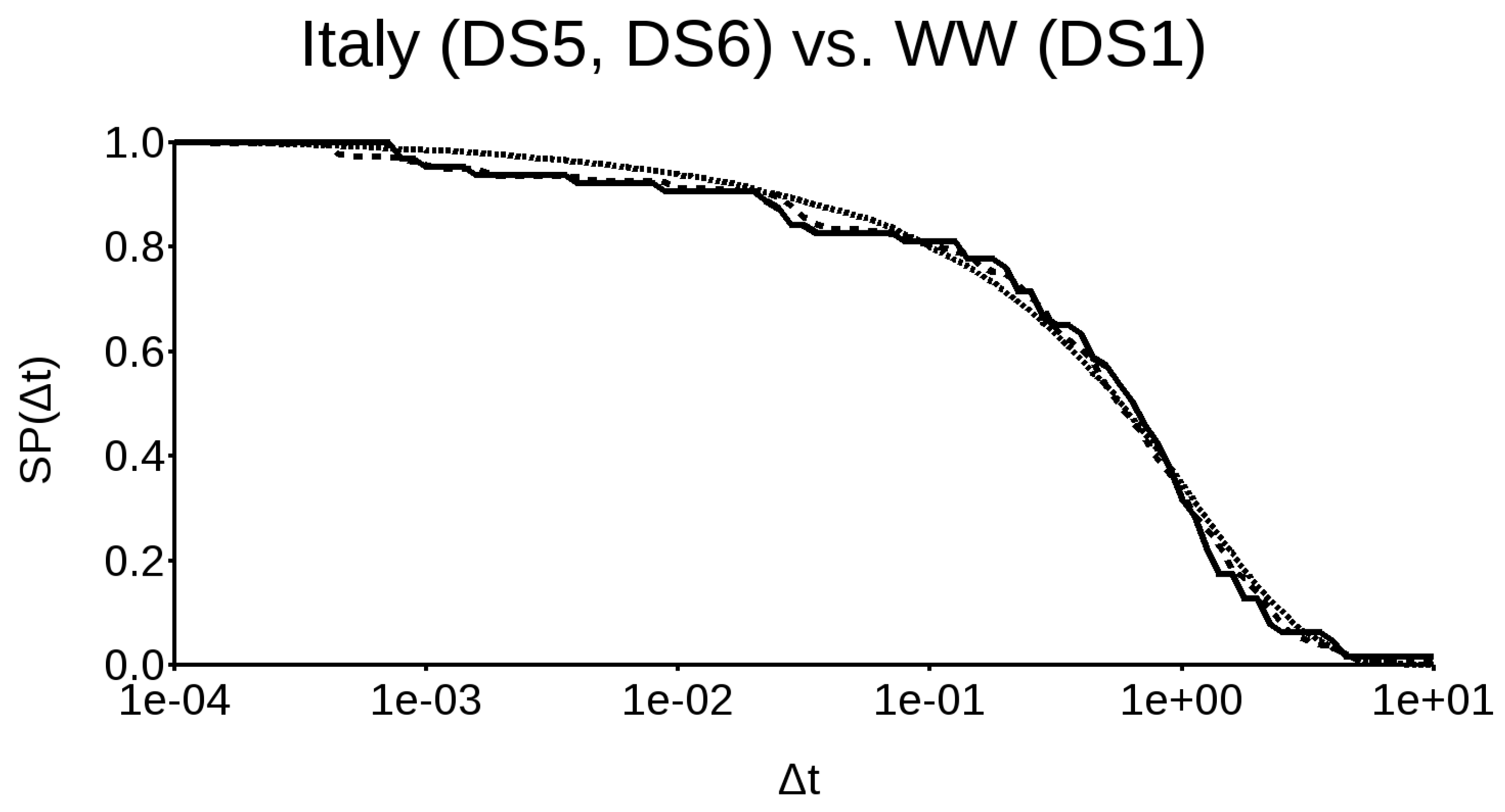
Figure 9.
Daily length (in days) of the 10% occurrence probability after each of the last seven major events that struck Italy. The dashed line refers to the date of occurrence of the following event. Gray areas correspond to the periods of most probable occurrence of the next large event.
Figure 9.
Daily length (in days) of the 10% occurrence probability after each of the last seven major events that struck Italy. The dashed line refers to the date of occurrence of the following event. Gray areas correspond to the periods of most probable occurrence of the next large event.


Table 1.
Date of occurrence of the seven last major events in Italy. The other columns are with respect to the previous event and the average from 1600 up to the current event, both in days.
Table 1.
Date of occurrence of the seven last major events in Italy. The other columns are with respect to the previous event and the average from 1600 up to the current event, both in days.
| Event Date | Previous Event (Days) | (Days) |
|---|---|---|
| 15 April 1978 | 709 | 2371 |
| 23 November 1980 | 953 | 2350 |
| 6 April 2009 | 10,360 | 2337 |
| 20 May 2012 | 1140 | 2301 |
| 24 August 2016 | 1557 | 2264 |
| 26 October 2016 | 64 | 2371 |
| 30 October 2016 | 3 | 2350 |
© 2020 by the author. Licensee MDPI, Basel, Switzerland. This article is an open access article distributed under the terms and conditions of the Creative Commons Attribution (CC BY) license (http://creativecommons.org/licenses/by/4.0/).
Share and Cite
MDPI and ACS Style
Harabaglia, P. Non-Poissonian Earthquake Occurrence Probability through Empirical Survival Functions. Appl. Sci. 2020, 10, 838. https://doi.org/10.3390/app10030838
AMA Style
Harabaglia P. Non-Poissonian Earthquake Occurrence Probability through Empirical Survival Functions. Applied Sciences. 2020; 10(3):838. https://doi.org/10.3390/app10030838
Chicago/Turabian StyleHarabaglia, Paolo. 2020. "Non-Poissonian Earthquake Occurrence Probability through Empirical Survival Functions" Applied Sciences 10, no. 3: 838. https://doi.org/10.3390/app10030838
Note that from the first issue of 2016, this journal uses article numbers instead of page numbers. See further details here.