Abstract
Surface finishing and polishing are important quality assurance processes in many manufacturing industries. A polished surface (low surface roughness) is linked with many useful properties other than providing an appealing gloss to the product, such as surface friction, electrical and chemical resistance, thermal conductivity, reflection, and product life. All these properties require an efficient polishing system working with the best machining parameters. This study analyzed the effects of the different input polishing parameters on the polishing efficiency and torque in the robotic polishing system for the circular-shaped workpieces (such as ring, cylinder, sphere, cone, etc.) by using the Taguchi method and analysis of variance (ANOVA). A customized rotatory passive gripper is designed to hold the watch bezel during polishing. Under the design of experiments (DOE) technique, Taguchi’s array is selected to find the optimized process parameters for polishing efficiency (based on surface roughness) and torque. Experimental results with the statistical analysis by signal-to-noise ratio and ANOVA (95% confidence level) confirms that the polishing force and tool speed are the most influencing parameter for polishing efficiency in the system. Linear regression equations are modeled for the polishing efficiency and torque. Finally, a confirmation test is conducted for the validation of the experimentation results against actual results.
1. Introduction
Surface finishing and polishing are important quality assurance processes in many manufacturing industries. Effective quality control can be achieved by meeting the predefined specific standards of the final product. Surface polishing is a complex process depending on various input polishing parameters. The output of this process is a smooth surface which can be characterized by plenty of parameters such as lay, surface roughness, and waviness. Many industries are using surface roughness and glossiness as the judgment factor to achieve smooth surfaces [1,2]. However, surface roughness is the most adopted parameter to quantify the surface finish [3,4,5,6]. Presently, in most polishing factories, the understanding and the knowledge of the well-experienced workers is a gauge for setting the machining parameters. On the contrary, some use a trial and error method to achieve the approximated values, especially if they are dealing with a new workpiece or adopting a new polishing system. However, such methods do not lead the system towards the optimal setting for economical polishing. For economical surface polishing, it is necessary that all the input factors work on the optimum level.
The design of experiments (DOE) is an organized approach to find out the effect of the input factors on the output of the process and help to optimize it. In other words, a DOE is an effective and economical method for experiment planning to achieve the desired results [7]. It offers statistical bases for analysis and helps to establish a conclusion. The idea of dealing with multiple factors of a process in an orderly manner is first presented by R. A. Fisher [7,8,9,10]. This method encourages the full factorial DOE which uses all set of possible combinations of factors. However, processes with a large number of factors can rapidly increase the number of experiments in full factorial design. To reduce the number of experiments, a limited number of experimental runs can be select by using other DOE approach such as Taguchi method.
Taguchi has presented a systematic method that efficiently selects the set of experiments from all possible combinations which are useful to optimize the output economically in terms of performance and quality [11,12,13,14,15]. This method uses orthogonal arrays which use the minimum number of experiments to extract the complete information about input parameters of the process. These experimental arrays are generally selected depending on the tradeoff between the cost (time or resources) of the experiments and the accuracy of the results [16].
Many studies have been used the Taguchi method to optimize the surface quality parameters (such as roughness) for the polishing process. Usually, the automated polishing process consists of several steps using various polishing input parameters such as abrasive grain sizes, no. of polishing cycles, feed rate, polishing force, and others. M. J. Tsai and J. F. Huang proposed the automatic polishing process step scheduling method with a compliant abrasive tool to select the optimal polishing parameters for different polishing steps [17]. An evaluation of the optimized parameters for the effective decrease in the surface roughness in each step is achieved by the Taguchi method. Another study [18] proposed the Taguchi DOE method to optimize the finishing conditions for the magnetic float polishing (MFP) technique to finish the silicon nitride balls for hybrid bearing applications. Reference [19] used orthogonal array () for finishing advanced ceramic balls using a novel eccentric lapping machine. It used the standard three-level array to analyze the ice fixed abrasive polishing on the single crystal silicon wafer for polishing parameters (polishing pressure, table velocity, eccentricity, and polishing time). Hsin-Te Liao at el. investigated the parameters for chemical mechanical polishing (CMP) processes in wafer manufacturing by the Taguchi method and designs of experiments (DOE) approach to optimize it [20]. In this study, the material removal rate and non-uniformity of surface profiles were selected as the quality targets. Besides optimal parameter achievement, several other methods have been used to improve the automated polishing process. Such methods include improvising of the tool path planning [21,22,23,24], controlled interaction between tool and surface [25,26,27], and the design of new polishing tools for specific or general type workpieces [28,29,30]. However, the optimization of parameters remains a very useful technique that can be implemented together with all these above-mentioned techniques to improve the automated polishing process [2].
This paper uses the orthogonal array of Taguchi design experiments. The analysis and optimization of the experimental results performed are based on a high signal to noise (S/N) ratio for high polishing efficiency (in terms of surface roughness) and low torque. For this experimental design, 18 experiments are conducted by various combinations of the levels of the control factors (startup torque of rotatory gripper, wheel speed, normal contact force, and gripper velocity). Moreover, the analysis of variance (ANOVA) is used to validate the results obtained from the Taguchi method and for the investigation of the performance of the individual parameter. Later, a mathematical model of polishing efficiency and the torque is developed by using regression analysis as a function of the control factors. Finally, an experimental verification test is conducted with the control factor levels predicted for the best polishing efficiency and torque.
2. Experimental Procedure
2.1. Workpiece and Polishing Tool
The workpiece used in this experimental study for testing the proposed polishing system setup is a watch bezel which is made of stainless steel (316). It is a popular material for its sparkling shine and is used in many exteriors. It is an excellent corrosion resistant and hard in nature. It is already treated with multiple sanding stages with different abrasive grits and now ready for final polishing with a buffing wheel that removed all remaining scratches and gave an astonishing gloss.
The selection of the polishing tool depends on numerous factors such as no. of workpiece per polishing tool, tool compliance, required surface quality, polishing time, and tool changing time [31]. In this study, a stitched cloth polishing wheel with a four-inch diameter (50 plies, 12-mm inner hole diameter) is used with dry polishing wax (P126) for the final polishing of the watch bezel. This stitched type polishing wheel has complete circles of sewing on the wheel in smaller diameter ranges. This type of sewing on the wheel provides firmness without losing flexibility. To enhance the wheel strength and width, two similar wheels are joined together that increased the overall width of the polishing wheel up to 30 mm.
2.2. Experimental Setup
Figure 1 shows the experimental setup for polishing the watch bezel by using ABB IRB 1200 6-axis industrial robot controlled by the IRC5 controller. It has 7 kg payload which is enough to support gripper and force sensor during polishing. A force feedback control system (Active contact flange by Ferrobotics; model ACF110-01) controlled by a separate setup is used to control the normal contact force between surfaces of the polishing wheel and watch bezel during interaction. For this controlled interaction, force sensor is attached with the passive rotatory gripper. Moreover, a torque sensor (rotating torque measuring device) is used between the polishing wheel and motor to observe the torque experienced by the motor during polishing. A digital display is used to show the experienced torque. Flex pendant with the small touch screen allows user interaction for multiple purposes such as uploading, running and modification of the program.
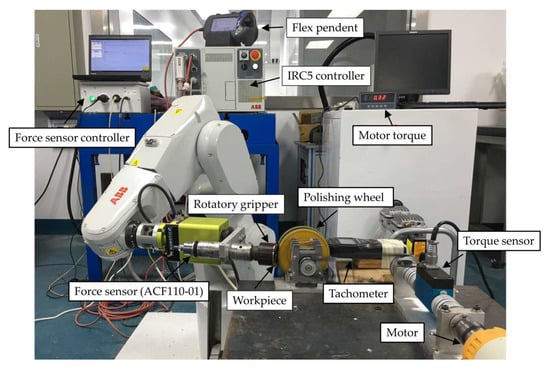
Figure 1.
Proposed system setup for the robotic polishing.
Figure 2a shows the top view of the specially designed rotatory gripper to hold the workpiece (watch bezel) during the polishing process using a closely stitched cotton polishing wheel. This passive gripper receives its driving force from the interaction of the rotating polishing wheel and is able to provide different start-up torques by adding weight to the gripper. This changing load provides different frictional values between tool and workpiece. The used ACF system for controlling the normal force is a hybrid force and position control system which is controlling the force and position in the direction normal to the polishing wheel surface. Figure 2b shows the isometric view of the watch bezel used in the experiments.
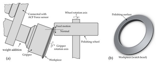
Figure 2.
Polishing wheel and workpiece: (a) Top view of the polishing wheel and workpiece interaction; (b) isometric view of the workpiece (watch bezel).
Figure 3 shows the different equipment used for the experimental analysis. A surface roughness tester (Mitutoyo, model: SJ-210) is used to evaluate the polishing surface. The torque sensor (Forsentek, model: FY02) is used for measuring the required polishing torque and tachometer for the wheel rotation speed.
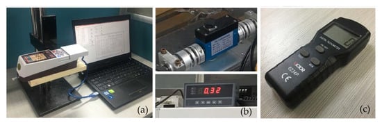
Figure 3.
Equipment used in experiments: (a) surface roughness tester (Mitutoyo, SJ-210); (b) torque sensor (Forsentek, FY02); (c) tachometer.
2.3. Taguchi Method and Polishing Parameters
Before designing the experiments using Taguchi’ orthogonal arrays, it is worth mentioning here that in surface polishing, it is always desired to remove less material to achieve the smooth surface as higher material removal can easily deform the shape of the workpieces, especially at the edges. Therefore, the target is to remove the peaks in the surface roughness profile of the surface to be polished, which is only possible with the optimal polishing force. Figure 4 shows the surface roughness height profile of the surface of the watch bezel before and after the initial polishing tests. Besides the surface roughness () of the height profile, skewness ), and kurtosis are also mentioned here because these parameters help to understand the distribution of the peaks and valleys present in height profile. Before polishing height profile have many high peaks and deep valleys ( = −0.505, and = 3.409). After the surface polishing, the height profile became highly negatively skewed ( = −1.530) because more high peaks are removed compared to the valleys. For the precise interaction workpiece is allowed to rotate upon wheel interaction to avoid the extreme frictional force. This interaction can be optimized by controlling the gripper’s rotational friction or moment of inertia (it is the amount of torque required to rotate a rigid body about its rotational axis). Moment of inertia depends on the mass of the body as , where m is mass and r is the distance from the pivoted point. Therefore, the rotational friction of the gripper can be control by adding friction to the axil or by adding the mass to the gripper. In this gripper, mass (circular ring with a mass of 0.303 Kg) is added to the rotational part of the gripper to change its load or startup torque or moment of inertia.
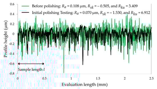
Figure 4.
Roughness height profile of the surface of the watch bezel.
Taguchi based DOE is used to analyze the effect of machining input parameters on the proposed system for the polishing of watch bezel. The input parameters are wheel rotation speed (ω), normal contact force (, gripper vibratory motion velocity , and gripper start-up torque (. These parameters are tested for polishing efficiency (PE) and polishing torque (T). Input polishing parameters for the system with its levels are shown in Table 1. To analyze the effect on the process two different levels are created by adding weight to the rotating part of the gripper as discussed previously. The polishing wheel speed and normal force are two important parameters that work collectively for economical polishing. Wheel speed is usually measured in surface feet per minute (SFPM) as: , where D is the wheel diameter and rpm is the rotation per minute.

Table 1.
Input polishing parameters and levels.
Depending on the initial testing, material removal requirement, related literature study [32], and the experiences of the experts working on the steel polishing, three levels are selected for the speed (3500, 4000, and 4500 rpm). In polishing particularly to achieve the mirror-like shine from the semi-polished surface, a higher material removing rate is avoided. Additionally, higher contact forces damage wheel shape, reduce its life, and increase power consumption (torque), which is not good for economical polishing. Therefore, the selected levels of the normal force for the experimental tests are 8 N, 12 N, and 16 N. The last input parameter is the feed rate or gripper speed (5 mm/s, 10 mm/s, and 15 mm/s) as shown in Figure 1. It offers an even polishing effect on the surface and enhances wheel life by not lingering it on the same point for a long time.
Taguchi based orthogonal array with mixed levels is selected to study the contribution each parameter on the polishing process (Table 2). In order to reduce the error margin, each of the eighteen experiments is repeated five times and for every experiment four reading for surface roughness are taken. The surface roughness before and after the experiment are measured to calculate Δ. Polishing efficiency (PE) is calculated as [2,17]
where A is the total polishing area, Δ is the reduction in the roughness, and is the polishing time. Area and time are constant so the PE depends on the roughness reduction. Here, input parameters are optimized for the highest polishing efficiency.
Table 2.
Orthogonal array
The core reason for the deprived production quality in any manufacturing or machining process is the variations in the process. These variations can be due to the change in conditions such as material quality, temperature, and any other process parameters. These changing variables (noise) are difficult to control or sometimes impossible. For the robust design, it is necessary to find the setting of the manageable process parameters which has the nominal effect of the noise on the product quality. Control and noise factors are a major part of the parameter design investigation which measures the interaction (signal to noise (S/N) ratio) between these factors. In robust design, three quality effecting influential parameters (factors) of the product or the process are signal factor (it directly influences the response of the product/process), noise factor (source of variation which is difficult/expensive to control), and control factor (it minimizes the system’s response sensitivity from the noise) [10] as shown in Figure 5.
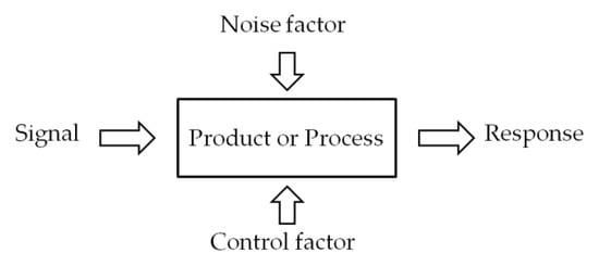
Figure 5.
Block diagram of the system input and output factors.
Depending on the target of the experiments, different S/N ratios can be selected. Under these different selections, S/N ratios quantify how the variation in the response happened relative to the target value [33]. Three different S/N characteristic formulations (conditions) are present in the following equations.
Smaller is the best:
Larger is the best:
Nominal is the best:
where y is the observed data, is its average, is its variance, and n is the number of observations. Equation (2) presents the S/N ratio for the condition (Smaller is the best) which requires the smallest possible performance value [10]. Similarly, Equation (3) shows S/R ratio for the condition (Larger is the best) for the largest possible performance values. The third S/N ratio condition is nominal is the best, S/N ratio for the case present in Equation (4). S/N ratio in this condition requires performance value to stay near to the selected target as much as possible. For this study, larger is the best is selected for the PE and smaller is the best is selected for the torque.
2.4. Analysis of Variance (ANOVA)
ANOVA is a statistical method used to compare the difference between means of groups. The results of this analysis are presented in the form of a table which shows the influence of the control factors in the experimental test. ANOVA table consists of various statistics such as sources (it contains control factors, error, and total of all sources), degree of freedom (DF) of data, sum of square (SS) of data, means sum of square (MS) of date, Fischer’s F distribution (F-value), p-value, and percentage contribution of the controlling factors. The detailed explanation of the items in the ANOVA table is as follows:
Source: It contains the control factors (between group or treatment), their interactions, error (within the group), and the total of all sources.
SS: It is the sum of squares of the data. The total sum of squares () is the sum of squares of the factors () and the sum of squares of the error () as:
where, and .
DF: It represents the degree of freedom of the data and can be represented similarly to the SS (Equation (6)). The total degree of freedom () can be calculated as n-1, where n is the total number of data. The degree of freedom of factors () and error () are k-1 and n-k respectably.
MS: It is the mean sum of the square of the data which can be calculated by dividing the SS by related DF. Mean sum of square of the factors and error can be calculates as = /k − 1, and = /n − k respectively.
F-value: It is also called the F-test which is a ratio of two variances and compares the factors. Variances are measures of how much the date is scattered from the mean. It can be calculated by dividing the mean sum of the square of the factor () by the error mean square () as:
p-value: It helps to define the significance of the results in a statistical test to accept or reject the null hypothesis. Depending on the significance, the p-value expresses between 0 and 1. Smaller value provides a strong indication for rejecting the null hypothesis. Typically this value keeps ≤ 0.05.
% contribution: It is the ratio of the sum of the squares () of the variable to the total sum of the square () of all the variables [34]. It shows the influence of the particular variable (factor) in terms of percentage on the response of the product/process as:
2.5. Regression
Regression is a statistical modeling process which establishes relation among dependent (response) and independent variables (input parameters or predictor). Regression can be modeled as linear and in polynomial relationships. The most common regression is linear regression, for which an investigator finds the linear function that most closely close to the data. The equation for the multiple linear regressions is shown in Equation (9).
where, is the constant value of the response (y) for the predictor (x) value 0. Additionally, it determines where the regression line intercepts the y-axis with the predictor variable(s) is zero. Depending on the relationship x can be a polynomial term. are the coefficients which determine the change in response for the one-unit change in the input parameter value.
3. Results and Discussion
3.1. Analysis of the Means and S/N Ratios of the Results
Polishing efficiency and torque were measured by the Taguchi design of experiments for the different factors as shown in Table 3. In order to minimize the error, each experiment is repeated four times. The total polishing time () for polishing of one workpiece was 60 s. Optimization of the control factors is performed by the calculated S/N ratios for the PE and T. The highest PE and the lowest T values are desirable for better system performance on lower production costs. Therefore, S/N condition higher the best for PE and lower the best for the T is used as in Equations (3) and (2) respectively.
Table 3.
Experimental results for polishing efficiency, and torque.
Table 4 shows the response tables of the average response of the S/N ratios, which analyze the effect of the control factors (, ω, ) on the response of PE and T. It reveals all the levels based on the S/N ratios for the control factors that provides highest PE as at level 1 (S/N = −2.451), ω at level 3 (S/N = −2.066), at level 3 (S/N = −1.312), and at level 1 (S/N = −2.642). Similarly, for the lowest T, the best factor levels and S/N ratios are at level 1 (S/N = 9.049), ω at level 1 (S/N = 9.398), at level 1 (S/N = 12.278), and at level 3 (S/N = 9.160). Delta and the rank determine which of these four factors has the greatest impact on the response. Delta measures the magnitude of the impact by subtracting the lowest average response value of a factor from its highest value. Rank assigns the order number to the factors in highest to lowest impact depending on the delta values. For PE, has highest impact (delta: S/N = 3.447, and rank = 1) and has lowest impact (delta: S/N = 0.246, and rank = 4). Likewise, for the T, also has the highest impact (delta: S/N = 6.164, and rank = 1), however has the lowest impact (delta: 0.018, S/N = 0.357, and rank = 4).
Table 4.
Response table for mean S/N ratios.
The graphical representation (main effects plot) of the levels of the factors in Table 4 is shown in Figure 6 and Figure 7. These main effect plots show the optimum values of the control factors to achieve the highest PE and lowest T. The main effect is called the difference in the means due to various levels within a factor. If the graph line is horizontal then there is no main effect present for the levels of a factor but the line with higher slop or difference between vertical points will have a higher main effect. For both polishing efficiency and torque, normal force shows the graphical lines with higher slopes, and therefore it has the highest main effect. The main goal of the experimentation is to find the control factor levels that minimize the noise factors on the responses. Optimal polishing parameters of the control factors for maximize the PE and minimizing the T can be easily determined from these graphs. The best level for each control factor was found according to the highest S/N ratio in the levels of those input parameters (control factors). The control factors range in the experiments for the is 0.019–0.02 Nm, for ω is 3500–4500 rpm, for is 8–16 N, and for is 5–15 mm/s. , 0.019 Nm; ω, 4500 rpm; 16 N, and 5 mm/s are best for the polishing efficiency and , 0.019 Nm; ω, 3500 rpm; 8 N, and 15 mm/s. The most significant factor is a force for both responses.
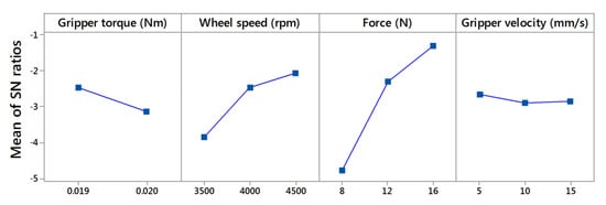
Figure 6.
Main effects plot of SN ratios for polishing efficiency.
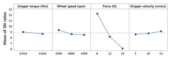
Figure 7.
Main effects plot of SN ratios for torque.
3.2. Analysis of ANOVA
The Taguchi method helped to find out the optimal number of experiments and provides a way to optimize the system through S/N ratios. For the further solidification of the results obtained in the Taguchi method based on S/N ratios, an ANOVA statistical model is used. Unlike the Taguchi method it calculates the percentage contribution of each factor involves. Table 5 and Table 6 shows the ANOVA table for the PE and T. The significance of control factors in ANOVA is determined by comparing the F values of each control factor. These tables were calculated with a 5% significance level and a 95% confidence level. If the p-value for the factor is greater than 0.05, then it will be considered as a non-significant factor. Therefore, based on the p-values of , p-value is not a significant parameter for the polishing efficiency. Similarly, (p-value = 0.000) is the only significant parameter for response of torque.
Table 5.
ANOVA table for polishing efficiency (PE).
Table 6.
ANOVA table for Torque (T).
The percentage contribution in the ANOVA tables shows the magnitude of the influence of the parameters calculated by Equation (8). The contribution of the gripper torque, tool speed, force, and feed rate for maximizing the polishing efficiency are 3.93%, 19.96%, 71.56%, and 0.57%, respectively. Similarly, for the polishing torque minimization, these percentages are 0.66%, 3.01%, 90.54%, and 1.12%. The most significant parameter for both responses is the normal contact force (71.56% for PE, and 90.54% for T). The percent of error was considerably low at 4.12% and 4.66% for PE and T respectively. Table 7 shows the cell mean of the control factors in ANOVA for PE and T. For polishing efficiency, the best input parameter are = 0.767 (level 1), ω = 0.802 (level 3), = 0.864 (level 3), and = 0.751 (level 1). Similarly for the T, the best input parameters are = 0.368 (level 1), ω = 0.350 (level 1), = 0.243 (level 1), and = 0.366 (level 3). Results from the ANOVA are well matched with the Taguchi method results for the best input parameters.
Table 7.
Cell mean of the control factor Response table for cell means.
3.3. Regression Analysis of Polishing Efficiency and Torque
In this research study, a relationship between two response variables and the four input variables are modeled and analyzed by using regression analysis. Two response variables are PE and T. Predictor or variables are control factors (, ω, , and ). Two linear regression equations are modeled for polishing efficiency and torque. Some important parameters to judge the regression models are R-sq (it describes, how much variation is present in the response), R-sq (adj) (it is a modified R-sq that has been adjusted for the number of expressions), and R-sq (pred) (how good the model predicts the response for new observations). For the good regression model, these values must be high. Equation (10) shows the linear regression for the polishing efficiency , which has R-sq = 91.47%, R-sq (adj) = 88.84%, and R-sq (pred) = 83.88%. Equation (11) shows the linear regression for Torque , which has R-sq = 94.34%, R-sq (adj) = 92.60%, and R-sq (pred) = 87.63%.
Figure 8a,b compares the experimental value (actual value) for the polishing efficiency and torque to the predicted ones achieved by the linear regression model which is closely matched with the actual values.
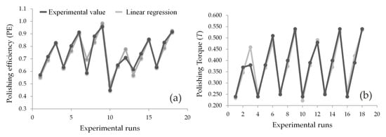
Figure 8.
Predicted results against experimental results: (a) for polishing efficiency; (b) for torque.
3.4. Confirmatory Test
In the last, a confirmatory test is conducted with the optimal input polishing parameters ( ω = 4500 rpm, =16 N, and = 5 mm/s) of the proposed system achieved previously by using Taguchi method and ANOVA. A comparison between the tested and the expected results from the linear regression model for the polishing efficiency and the torque is presented in in Table 8. A good agreement is found between the experimental and the predicted results that confirm that the experimentation based on the Taguchi method is properly conducted to explore the system response for the different levels of the input parameters (control factors). Figure 9 shows the watch bezel before and after the polishing using optimized polishing parameters on the selected polishing area.
Table 8.
Conformation test results for the optimal polishing parameters.
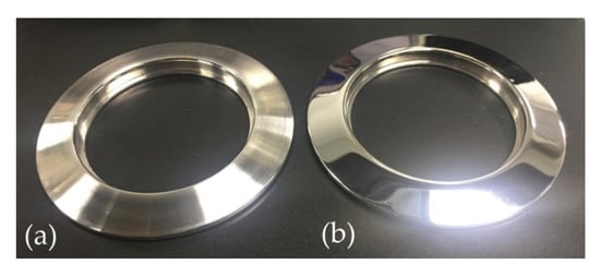
Figure 9.
Watch bezel: (a) before polishing and (b) after robotic polishing.
4. Conclusions
This study presented a detailed analysis of the input polishing parameters (startup torque of rotatory gripper, wheel rotational speed, normal contact force, and gripper vibratory motion velocity) on the polishing efficiency and torque for the proposed robotic polishing system by using Taguchi design of experiments (DOE). The proposed robotic polishing system is tested for the watch bezel. Experimental results analysis by signal to noise ratios optimizes the responses and closely matched with the ANOVA results that further legitimized the experimental study. Additionally, regression line equations are added to model the response behavior of the polishing efficiency and torque for the input polishing parameters. Finally, a confirmation test is conducted for affirming the authenticity of the experimental results and to check the regression model by comparing the experimental result and predicted result at optimal levels of the input factors. From the above results, analysis, and discussion, the following conclusions can be drawn:
- (a)
- Robot polishing is a challenging task that requires precision, as well as the consideration of polishing surface coverage, controlled polishing force, and best polishing parameters. The presented polishing system with optimal polishing parameters is effective and finishes the polishing job in a short time with precision.
- (b)
- The S/N ratios analysis from the Taguchi method shows the best levels of the control factors for highest polishing efficiency (PE = 0.943) as: start-up torque of rotatory gripper = 0.019 Nm (S/N = −2.451), wheel speed = 4500 rpm (S/N = −2.066), normal contact force = 16 N (S/N = −1.312), and gripper velocity = 5 mm/s (S/N = −2.642). Similarly, the best levels of the control factors for the minimum torque (T = 0.47 Nm) as: start-up torque of rotatory gripper = 0.019 Nm (S/N = 9.049), wheel speed = 4500 rpm (S/N = 9.398), normal contact force = 16 N (S/N = 12.278), and gripper velocity = 5 mm/s (S/N = 9.160).
- (c)
- According to the ANOVA statistical model, selected optimal levels for each control factors are same as in Taguchi method. It further determines the ranks and % contributions of the control factors for polishing efficiency (: rank = 1 and % = 71.56, ω: rank = 2 and % = 19.96, : rank = 3 and % = 3.93, and : rank = 4 and % = 0.57) and torque (: rank = 1 and % = 90.54, ω: rank = 2 and % = 3.01, : rank = 3 and % = 1.12, and : rank = 4 and % = 0.66).
- (d)
- Polishing efficiency is given higher preference over polishing torque, therefore the overall system input parameters for good polishing efficiency and torque are as: startup torque of rotatory gripper = 0.019 Nm, wheel speed = 4500 rpm, normal contact force = 16 N, and gripper velocity = 5 mm/s.
- (e)
- The most significant control factor which contributes more to the polishing process in this system is the normal contact force applied by the polishing wheel following the wheel speed, gripper torque, and gripper vibratory velocity. Gripper velocity is comparatively less significant factor in achieving the good polishing surface in a short time but it is useful in a way that it uniformly distributes the polishing effect on the surface area and safe the polishing wheel from damage and shape deformation by avoiding lingering it at one point for a long time. Therefore, the correct combination of the force, speed, and gripper torque can achieve the desired level of the surface quality in a short time.
- (f)
- Robotic polishing is an advantageous process which offers productivity, error minimization, product consist quality. Additionally, it can protect humans from the unhealthy environment of the polishing workplace. With the optimization of the process parameters, robotic polishing can further improve the polishing process. This study used some important but limited number of input polishing parameters and their levels to shows the effect on the polishing process. In the future, some other factors will be included, such as polishing time, different polishing tools, etc.
Author Contributions
I.M., K.H., and R.D. contributed to the main idea of this paper; I.M. performed the experiments, analysed the data and wrote the paper; K.H. is the project principal investigator; R.D. gave some system improvement suggestion and the paper structure, Z.L. and F.Z. gave some data analysis and revision suggestions. All authors have read and agreed to the published version of the manuscript.
Funding
This research was supported by Guangdong Science and Technology Planning Project (2017B090914004) and CAS-HK Joint Laboratory of Precision Engineering. Author (Imran Mohsin) acknowledges CAS-TWAS President’s Fellowship for sponsoring his Ph.D. at the University of Chinese Academy of Sciences, Beijing, 100049, China.
Conflicts of Interest
The authors declare no conflicts of interest.
References
- Li, H.; Li, X.; Tian, C.; Yang, X.; Zhang, Y.; Liu, X.; Rong, Y. The simulation and experimental study of glossiness formation in belt sanding and polishing processes. Int. J. Adv. Manuf. Technol. 2016, 90, 199–209. [Google Scholar] [CrossRef]
- Mohsin, I.; He, K.; Li, Z.; Du, R. Path Planning under Force Control in Robotic Polishing of the Complex Curved Surfaces. Appl. Sci. 2019, 9, 5489. [Google Scholar] [CrossRef]
- Kayahan, E.; Oktem, H.; Hacizade, F.; Nasibov, H.; Gundogdu, O. Measurement of surface roughness of metals using binary speckle image analysis. Tribol. Int. 2010, 43, 307–311. [Google Scholar] [CrossRef]
- Mahdavinejad, R.A.; Bidgoli, H.S. Optimization of surface roughness parameters in dry turning. J. Achiev. Mater. Manuf. Eng. 2009, 37, 571–577. [Google Scholar]
- Gold, G.; Helmreich, K.A. Physical Surface Roughness Model and Its Applications. IEEE Trans. Microw. Theory Tech. 2017, 65, 3720–3732. [Google Scholar] [CrossRef]
- Gadelmawla, E.; Koura, M.; Maksoud, T.; Elewa, I.; Soliman, H. Roughness parameters. J. Mater. Process. Technol. 2002, 123, 133–145. [Google Scholar] [CrossRef]
- Antony, J. Chapter Fundamentals of Design of Experiments. In Design of Experiments for Engineers and Scientists; Antony, J., Ed.; Elsevier: Amsterdam, The Netherlands, 2014; pp. 7–17. [Google Scholar] [CrossRef]
- Yates, F. Sir Ronald Fisher and the Design of Experiments. Biometrics 1964, 20, 307. [Google Scholar] [CrossRef]
- Stanley, J.C. The Influence of Fisher’s “The Design of Experiments” on Educational Research Thirty Years Later. Am. Educ. Res. J. 1966, 3, 223–229. [Google Scholar] [CrossRef]
- Rao, S.; Samant, P.; Kadampatta, A.; Shenoy, R. An Overview of Taguchi Method: Evolution, Concept and Interdisciplinary Applications. Int. J. Sci. Eng. Res. 2013, 4, 621–626. [Google Scholar]
- Kim, K.-S.; Jung, K.T.; Kim, J.-M.; Hong, J.-P.; Kim, S.-I. Taguchi robust optimum design for reducing the cogging torque of EPS motors considering magnetic unbalance caused by manufacturing tolerances of PM. IET Electr. Power Appl. 2016, 10, 909–915. [Google Scholar] [CrossRef]
- Sorgdrager, A.J.; Wang, R.-J.; Grobler, A.J. Retrofit design of a line-start PMSM using the Taguchi method. In Proceedings of the 2015 IEEE International Electric Machines & Drives Conference (IEMDC), Coeur d’Alene, ID, USA, 10–13 May 2015; pp. 489–495. [Google Scholar]
- Omekanda, A. Robust torque and torque-per-inertia optimization of a switched reluctance motor using the Taguchi methods. IEEE Trans. Ind. Appl. 2006, 42, 473–478. [Google Scholar] [CrossRef]
- León, R.V.; Shoemaker, A.C.; Kacker, R.N. Performance measures independent of adjustment: An explanation and extension of Taguchi’s signal-to-noise ratios. Technometrics 1987, 29, 253–265. [Google Scholar] [CrossRef]
- Jeyapaul, R.; Shahabudeen, P.; Krishnaiah, K. Quality management research by considering multi-response problems in the Taguchi method—A review. Int. J. Adv. Manuf. Technol. 2005, 26, 1331–1337. [Google Scholar] [CrossRef]
- Kacker, R.N.; Lagergren, E.S.; Filliben, J.J. Taguchi’s Orthogonal Arrays Are Classical Designs of Experiments. J. Res. Natl. Inst. Stand. Technol. 1991, 96, 577–591. [Google Scholar] [CrossRef] [PubMed]
- Tsai, M.J.; Huang, J.F. Efficient automatic polishing process with a new compliant abrasive tool. Int. J. Adv. Manuf. Technol. 2006, 30, 817–827. [Google Scholar] [CrossRef]
- Jiang, M.; Komanduri, R. Application of Taguchi method for optimization of finishing conditions in magnetic float polishing (MFP). Wear 1997, 213, 59–71. [Google Scholar] [CrossRef]
- Kang, J.; Hadfield, M. Parameter optimization by Taguchi methods for finishing advanced ceramic balls and using a novel eccentric lapping. J. Eng. Manuf. 2001, 215, 69–78. [Google Scholar] [CrossRef]
- Liao, H.-T.; Shie, J.-R.; Yang, Y.-K. Applications of Taguchi and design of experiments methods in optimization of chemical mechanical polishing process parameters. Int. J. Adv. Manuf. Technol. 2007, 38, 674–682. [Google Scholar]
- Tam, H.-Y.; Lui, O.C.-H.; Mok, A.C. Robotic polishing of free-form surfaces using scanning paths. J. Mater. Process. Technol. 1999, 95, 191–200. [Google Scholar] [CrossRef]
- Rososhansky, M.; Xi, F. Coverage based tool-path planning for automated polishing using contact mechanics theory. J. Manuf. Syst. 2011, 30, 144–153. [Google Scholar] [CrossRef]
- Kharidege, A.; Ting, D.T.; Yajun, Z. A practical approach for automated polishing system of free-form surface path generation based on industrial arm robot. Int. J. Adv. Manuf. Technol. 2017, 93, 3921–3934. [Google Scholar] [CrossRef]
- Mohsin, I.; He, K.; Du, R. Robotic Polishing of Free-Form Surfaces with Controlled Force and Effective Path Planning. ASME Int. Mech. Eng. Congr. Expos. 2018, 5, 87371. [Google Scholar]
- Oba, Y.; Kakinuma, Y. Tool Posture and Polishing Force Control on Unknown 3-Dimensional Curved Surface. Int. Manuf. Sci. Eng. Conf. 2016, 1, 8762. [Google Scholar]
- Mohsin, I.; He, K.; Cai, J.; Chen, H.; Du, R. Robotic polishing with force controlled end effector and multi-step path planning. In Proceedings of the 2017 IEEE International Conference on Information and Automation (ICIA), Macau, China, 18–20 July 2017; pp. 344–348. [Google Scholar]
- Jinno, M.; Ozaki, F.; Yoshimi, T.; Tatsuno, K.; Takahashi, M.; Kanda, M.; Tamada, Y.; Nagataki, S. Development of a force controlled robot for grinding, chamfering and polishing. In Proceedings of the 1995 IEEE International Conference on Robotics and Automation, Nagoya, Japan, 21–27 May 1995; pp. 1455–1460. [Google Scholar]
- Wang, C.; Wang, Z.; Wang, Q.; Ke, X.; Zhong, B.; Guo, Y.; Xu, Q. Improved semirigid bonnet tool for high-efficiency polishing on large aspheric optics. Int. J. Adv. Manuf. Technol. 2016, 88, 1607–1617. [Google Scholar] [CrossRef]
- Mohammad, A.E.K.; Hong, J.; Wang, D.; Guan, Y. Synergistic integrated design of an electrochemical mechanical polishing end-effector for robotic polishing applications. Robot. Comput.-Integr. Manuf. 2019, 55, 65–75. [Google Scholar] [CrossRef]
- Perez-Vidal, C.; Gracia, L.; Sanchez-Caballero, S.; Solanes, J.E.; Saccon, A.; Tornero, J. Design of a polishing tool for collaborative robotics using minimum viable product approach. Int. J. Comput. Integr. Manuf. 2019, 32, 848–857. [Google Scholar] [CrossRef]
- Arunachalam, A.P.S.; Idapalapati, S.; Subbiah, S. Multi-criteria decision making techniques for compliant polishing tool selection. Int. J. Adv. Manuf. Technol. 2015, 79, 519–530. [Google Scholar] [CrossRef]
- Metal Finishing Systems l 1-800-747-2637, Introduction to Buffing. Available online: http://www.metalfinishingsystems.com/ (accessed on 28 October 2018).
- Gopalsamy, B.M.; Mondal, B.; Ghosh, S. Taguchi method and ANOVA: An approach for process parameters optimization of hard machining while machining hardened steel. J. Sci. Ind. Res. 2009, 68, 686–695. [Google Scholar]
- Shahri, H.R.F.; Akbari, A.A.; Mahdavinejad, R.; Solati, A. Surface hardness improvement in surface grinding process using combined Taguchi method and regression analysis. J. Adv. Mech. Des. Syst. Manuf. 2018, 12, JAMDSM0049. [Google Scholar] [CrossRef]
© 2020 by the authors. Licensee MDPI, Basel, Switzerland. This article is an open access article distributed under the terms and conditions of the Creative Commons Attribution (CC BY) license (http://creativecommons.org/licenses/by/4.0/).