Article

Gait Recognition via Deep Learning of the Center-of-Pressure Trajectory

by
Philippe Terrier
1,2
1
Haute-Ecole Arc Santé, HES-SO University of Applied Sciences and Arts Western Switzerland, 2000 Neuchâtel, Switzerland
2
Department of Thoracic and Endocrine Surgery, University Hospitals of Geneva, 1205 Geneva, Switzerland
Appl. Sci. 2020, 10(3), 774; https://doi.org/10.3390/app10030774
Submission received: 3 December 2019 / Revised: 8 January 2020 / Accepted: 20 January 2020 / Published: 22 January 2020
(This article belongs to the Special Issue Deep Learning-Based Biometric Recognition)

Abstract

:

Featured Application

Sensing floors combined with pattern recognition and deep learning could identify individuals by the way they unfold their footsteps on the ground.

Abstract

The fact that every human has a distinctive walking style has prompted a proposal to use gait recognition as an identification criterion. Using end-to-end learning, I investigated whether the center-of-pressure (COP) trajectory is sufficiently unique to identify a person with high certainty. Thirty-six adults walked for 30 min on a treadmill equipped with a force platform that continuously recorded the positions of the COP. The raw two-dimensional signals were sliced into segments of two gait cycles. A set of 20,250 segments from 30 subjects was used to configure and train convolutional neural networks (CNNs). The best CNN classified a separate set containing 2250 segments with an overall accuracy of 99.9%. A second set of 4500 segments from the six remaining subjects was then used for transfer learning. Several small subsamples of this set were selected randomly and used to fine tune the pretrained CNNs. Training with two segments per subject was sufficient to achieve 100% accuracy. The results suggest that every person produces a unique trajectory of underfoot pressures while walking and that CNNs can learn the distinctive features of these trajectories. By applying a pretrained CNN (transfer learning), a couple of strides seem enough to learn and identify new gaits. However, these promising results should be confirmed in a larger sample under realistic conditions.

1. Introduction

Human beings move through their environment using repetitive movements of the lower limbs, such as walking or running. The sequence of these movements constitutes one’s gait. One gait cycle (or stride) is created by the alternation of stance and swing phases performed by the legs. The gait pattern is constrained by biomechanical and energetic factors [1]. Furthermore, each individual has a unique gait signature that can be used for identification purposes, in a process known as gait recognition [2]. The most interesting aspect of gait recognition is that it can identify subjects without their knowledge or approval, contrary to other biometric methods such as fingerprint or iris recognition.
Video-based methods dominate the field of gait recognition [3,4]. Researchers can benefit from numerous easily available video databases [5], the largest of which contains more than 10,000 individuals [6]. Recent advances show a recognition rate of between 90% and 95% in optimal viewing conditions; but the accuracy decreases under challenging conditions (such as occlusions, view variations, or appearance changes) [4]. Wearable inertial sensors have also been proposed for recognizing gait [7,8]. These sensors are used extensively in biomedical applications for gait analysis, and, therefore, significantly aid research efforts [9]. High recognition rates (>95%) have been observed under laboratory conditions [10], but a lower accuracy (~70%) has been reported in more realistic datasets [11].
Analyzing the force a walking individual applies to the ground has also been proposed for identifying people, an approach referred to as footstep recognition [12]. Different gait features can be extracted through force sensors embedded in the floor, including the temporal sequence of the ground reaction force (GRF) [13,14,15], the shape of the foot on the ground (footprint) [16], and the trajectory of the center of pressure (COP) [17]. The COP is the point at which the resulting vertical force is applied (i.e., the integrated vectorial pressure field). Promising results have been obtained, with classification rates higher than 95% [15,16] (see also Section 2); however, the number of footstep recognition studies is still low, particularly those that include a COP analysis. COP trajectory has never been used alone for identification and verification aims. In addition, most of the footstep recognition studies included only a few individuals performing a limited number of strides [2,12].
Recognizing people through their gaits relies on the analysis of multiple complex features. Neural networks are therefore helpful for this task [18]. Convolutional neural networks (CNNs) have been used with great success for video-based gait recognition [19,20]. CNNs are especially well suited for working with images as a result of their strong spatial dependencies in local regions and a substantial degree of translation invariance. Similarly, time series can exhibit locally correlated points that are invariant with time shifts. The successful use of deep CNNs for the classification of uni-dimensional or multidimensional time series has been attested [21,22]. Like for image classification, CNNs can extract deep features from a signal’s internal structure. CNNs are potent tools for bypassing feature engineering in signal processing tasks (end-to-end learning) [22]. However, CNNs, like other artificial neural networks, require hundreds of examples in each class for efficient learning; therefore, they have not been applied in footstep recognition studies so far due to the difficulty of collecting many strides using sensing floors or force platforms.
The innovative idea behind this study was to use an instrumented treadmill equipped with a force platform to record hundreds of consecutive strides. The recorded COP trajectories were then harnessed to identify individuals. I applied state-of-the-art CNNs and supervised end-to-end learning. The feature extraction capabilities of CNNs were used to classify individual gaits. The objective was to provide a proof-of-concept for the notion that measuring the COP alone can be used for biometric purposes. First, I assessed the classification accuracy of the method based on many strides (>500 per participant) in both identification and verification scenarios. Second, I used transfer learning to explore whether new gaits could be successfully classified when studying a couple of consecutive strides only, and to analyze accuracy changes when extra individuals are added to the dataset.

2. Related Works

In 2004, Jung et al. [17] suggested combining static and dynamic foot pressure features to identify walking individuals. They used a mat containing 40 × 80 pressure sensors (1 × 1 cm2 resolution) to record footprints and COP trajectories and collected one-step footprints from 11 participants. Forty footprints were recorded from each subject for two months. An overall classification accuracy of 98.6% was obtained using the hidden Markov model and Levenberg–Marquart learning methods. One strength of the study was that data were recorded over a long period of time and tended to demonstrate that foot pressure features are time invariant to a substantial degree. The study’s limitations included the small sample size and the fact that the subjects had to walk barefoot, making the method difficult to apply in practice.
In an article published in 2007, Suutala and Röning described a method for using a pressure-sensitive floor to identify individuals [18]. They covered the floor of their research laboratory with 100 m2 of an electro-mechanical film sensitive to pressure and collected gait pressure data from 10 individuals. The researchers focused on the pressure intensity profiles, rather than on pressure trajectories or foot shape. They applied several classifying algorithms, of which support vector machines and multilayer perceptrons were the most accurate. The most outstanding finding was that 95% classification accuracy was achieved when multiple features collected from several consecutive steps were combined. Despite the small sample, this study demonstrated the technical feasibility of using an instrumented (sensing) floor for biometric recognition.
In their 2012 study, Pataky et al. [16] analyzed dynamic foot pressure patterns through plantar pressure imaging using a pedography platform that recorded footprints with 5 mm resolution. They recruited 104 individuals and collected 1040 barefoot steps. Several pre-features characterizing the pressure patterns where extracted, and a dimensionality reduction technique was used. A one-fold nearest-neighbor classifier was applied with cross-validation. The results show that the best feature was the pressure–time integral (PTI), with a classification rate of 99.6%. Overall, this study demonstrated that plantar pressure patterns are highly unique among individuals. The main practical limitation was that they investigated unshod walking.
In 2015, Connor studied foot pressure data collected from 92 subjects walking either unshod or shod on a pressure mat (255 × 64 pressure sensors) [23]. The purpose was to evaluate the classification and identification performance under three scenarios: (1) a “barefoot” scenario, in which the recognition system classifies only barefoot data; (2) a “same shoe” scenario, in which the system classifies footsteps of subjects wearing the same footwear throughout; and (3) a “different shoe” scenario, in which the system learns from examples of individuals walking with one type of footwear, and then evaluates footsteps when they walked with a different type of footwear. Connor then assessed many pressure-derived features and combinations thereof, including COP trajectories, GRF timing, footprint images, and general gait features. The results reveal that for the most difficult scenario (i.e., #3), it was possible to achieve a classification accuracy of 90.5%. Interestingly, COP parameters were among the most important features for an optimal classification in both shod scenarios (#2 and #3). In addition, gait metrics—such as cadence, step length, toe-out angle, and foot length—also played a substantial role. In short, this study demonstrated that COP trajectory might be appropriate for classifying shod walking gaits.

3. Materials and Methods

3.1. Data Collection and Pre-Processing

The data used in the present study were collected by the author in a previous study aimed at analyzing the influence of voluntary synchronization to external sensory cues on gait variability [24,25]. Thirty-six healthy adults participated in the study, 14 men and 22 women. The means and standard deviations of their individual characteristics were age: 33 years (10), body height: 1.72 m (0.08), and body mass: 66 kg (13). The experiment consisted of 30 min of treadmill walking under three cueing conditions—no cueing, auditory cueing, and visual cueing. The participants wore their customary shoes, but high heels were forbidden. The treadmill was instrumented with a force platform consisting of six load cells that retrieved the intensity and the position of the vertical force exerted by the subject walking on the treadmill surface [26,27].
On a treadmill, the COP trajectory of a walking individual has a typical butterfly-like shape [28], as shown in Figure 1. The “wings” of the butterfly correspond to the stance on a single foot, whereas the central crossing corresponds to the double-support phase when the body weight passes from one foot to the other. For a dynamical representation of the process, refer to a short video published in the supplementary material of a previous article [29].
The 500 Hz two-dimensional (2-D) positional signals were low-pass filtered at 30 Hz and down sampled to 50 Hz. Each stride was identified in the raw signals [24,26]. Five-hundred strides were kept for each cueing condition and each participant. These 500-stride time series were resampled to a uniform length of 20,000 samples; that is, 40 samples per stride. The aim was to standardize the average stride duration among participants. Thus, the dataset contained three 2-D signals of 20,000 sample length for each of the 36 participants, for a total of 54,000 strides.
Each 2-D signal of 20,000 samples was split into three parts: the first 16,000 samples were added to the training set, the next 2000 samples to the development set (dev set), and the last 2000 samples to the test set. The signals were stacked across subjects and conditions in arrays of three columns corresponding to the x-axis, the y-axis and the subject’s identification (ID) number (1–36).
Finally, a non-overlapping sliding window algorithm sliced the arrays into small segments of 80 samples each (i.e., two strides, or four steps). Four random examples of these segments are shown in Figure 2. Each segment was labeled with the subject’s ID, which was converted into a categorical format. Two ensembles of sets were created, the first for developing and testing the CNN models and containing the data of 30 subjects (18,000 segments in the training set and 2250 segments in the dev and test sets) and the second for transfer learning, containing the data of six subjects (4050 segments in the training set, and 450 segments in the test set).

3.2. Software and Data Availability

GPU computing, with Tensorflow and Keras on Python 3.6, was used for CNN development. Other Python libraries used were Pandas, Numpy, Hyperopt, Hyperas, Matplotlib, and Scikit-learn. Some preliminary steps (raw signal filtering) were computed using MATLAB (Mathworks, Natick, USA). The raw data are available on FigShare [30]. The source code of the Python scripts can be obtained, and a reproducible run can be performed, on CodeOcean [31].

3.3. CNN

The overall network architecture is shown in Figure 3. I designed a CNN based on stacked one-dimensional (1-D) convolutional layers systematically followed by batch normalization [32] (not shown in Figure 3 for the sake of simplicity). Zero padding was used to ensure identical input/output sizes among layers. Maximum pooling layers were used to reduce dimension (Figure 3). I applied a CNN architecture that included skip connections; that is, a ResNet-like architecture [33], which has also been advocated for time series classification [22]. These shortcut paths between non-consecutive layers allowed for a better flow of information in a deep CNN, preventing in part the issue of vanishing/exploding gradients [34]. When shortcuts required dimension adjustments, one-fold convolution layers were applied with the appropriate number of filters (depth adjustment) or adjusted stride (temporal reduction). Nonlinearities were introduced via activation layers interleaved as recommended for the ResNet architecture (Figure 3).
In addition to the standard 1-D convolution layers, I tested whether depthwise separable 1-D convolution layers could provide a valuable alternative (Xception architecture [35]), hereafter referred to as sepCNN. These layers combine pointwise and depthwise convolutions, resulting in a factorized version of standard convolutions. SepCNNs use fewer parameters and are computationally more efficient [36], possibly a major advantage for practical applications. I used a similar architecture for both CNNs and sepCNNs, but their hyperparameters were tuned independently (see Section 3.4).
The loss function was categorical cross-entropy. The Nadam algorithm was chosen as the mini-batch gradient descent optimizer [37]. Nadam is a variant of the classical Adam algorithm [38], but with Nesterov momentum [39]. The recommended parametrization was used. The models were fitted using a mini-batch size of 256. The metric was overall accuracy (correct classification rate), i.e., the number of segments assigned to the correct person over the total number of segments.

3.4. Hyperparameter Tuning and Model Testing

Table 1 summarizes how the CNN hyperparameters were tuned. Regarding the model architecture, both the number of filters and the number of intermediate blocks (Figure 3) were adjusted. I also evaluated two different approaches for the final layers—the first using a classical combination of dense–dropout–softmax layers, and the second using a global average pooling layer [40] preceding the softmax layer.
Regarding activation, four algorithms were tested: ReLU [41], LeakyReLU [41], PReLU [42], and trainable Swish [43]. Swish is a recent algorithm, similar to the sigmoid-weighted linear unit proposed in [44], but with a trainable parameter. Regarding convolutional layer initialization, two algorithms were tested, the so-called Glorot-normal (Xavier-normal, [45]) and the He-normal [42]. Regarding L2 regularization, the optimal weight decay (λ) was searched for between 10−7 and 10−3. Finally, the optimal initial learning rate was searched for between 0.1 and 2 times the recommended value of 0.02; that is, between 0.002 and 0.04.
Bayesian optimization was used to search through the hyperparameter space. More precisely, I applied the tree of Parzen estimator (TPE) algorithm [46], as implemented in the Hyperopt library [47], and its Keras wrapper, Hyperas [48]. The overall accuracy on the dev set was used as the metric. Three-hundred trials were run and the combination that provided the highest accuracy was chosen.
A final training set was built by concatenating the train and dev sets. The accuracy of the best setting (Table 1) was assessed in the test set. An early-stopping algorithm was applied to reduce the training time. The assessment was repeated 10 times to take model stochasticity into account (Table 2).

3.5. Transfer Learning

The objective was to analyze the ability of the models to generalize on new—not previously learned—gaits. The first aim was to find the minimal number of strides required to tune a pretrained model for a correct classification of gaits of previously unseen individuals. Indeed, for future efficient applications, it is important to know whether gaits can be learned based on only a few strides. The second aim was to assess the model’s accuracy when extra individuals were added to the dataset.
The gait data from the six subjects not included in the model development were used. I applied the principles of transfer learning; the best models trained on the 30 subjects were fine-tuned based on the new gait data. First, most model parameters were frozen. That is, their trainable attributes were set to false; only the weights of the last two convolutional layers, and the parameters of the batch normalization layers, were kept trainable (see Figure 3). The output (softmax) layer was then replaced with a new layer with six neurons to match the new classification task. Regarding optimization, the learning rate was set to 0.0002 for the fine-tuning of the weights of the last layers.
To investigate the discriminative power of the new model, the output of its untrainable part and the output of the two trainable layers, were analyzed using t-distributed stochastic neighbor embedding (t-sne, Scikit-Learn implementation) [49]. T-sne is a nonlinear dimensionality reduction algorithm that embeds high-dimensional data in a low-dimensional space of two dimensions for the purpose of visualization. Here, t-sne helped to visualize whether the segments of each individual were clustered together. New CNN and speCNN models were trained with the 4050 segments of the training set (10 epochs, batch size = 32) and then inferred on the 450 segments of the test sets. T-sne reduced the dimension of the flattened layer outputs to two dimensions (Figure 4).
The new models were then trained and tested on very small samples, as follows. From the full test set containing 450 segments, 60 were randomly selected (10 per subject). Next, a variable number of random segments were drawn from the training set of 4050 segments—6, 12, 30, or 60; that is, 1, 2, 5, or 10 per subject, respectively. Finally, the overall accuracy of the test set was computed. Fifty repetitions of this procedure were conducted for each segment number (for a total of 200 repetitions). Boxplots were used to show result distributions (Figure 5).
To fulfill the second objective, a dataset containing all the available data was built; that is, 108,000 footsteps divided into 27,000 segments (24,300 in the training sets, 2700 in the test set) from 36 individuals. The best CNN and sepCNN were modified for the new classification task: their 30-neuron last layers were replaced with 36-neuron dense ones. Only the last two convolutional layers were set to trainable. The accuracy was tested in 10 trials (Table 2).

3.6. Verification

In most biometric applications, the goal is not necessarily to identify an individual but rather to verify whether an individual is an authorized user or not. To test this type of verification scenario, 100 different training and test sets were built to challenge the best CNN in verification tasks. First, a full training set including 48,500 strides (24,250 segments) of the 36 participants was gathered. An independent test set including 5500 strides (2750 segments) was also built for testing the performance of the classifier. The segment labels identifying each participant (ID 1 to 36) were modified as follows. Each participant could be considered an authorized user (label = 1) or an unauthorized user (label = 0); the repartition between authorized users and unauthorized users was randomly chosen. Four different levels of repartition were chosen—10 authorized users vs. 26 unauthorized users, 15 vs. 21, 20 vs. 16, and 25 vs. 11. Twenty-five repetitions for each repartition level were performed, each repetition including a random assignment of individuals between groups. Like for transfer learning (see above), the best pre-trained CNN was modified for the new classification task. The CNN weights were frozen, except those of the two last convolutional layers. Given the binary nature of the classification task, the output layer was replaced with a logistic classifier (sigmoid activation). The mini-batch size was 128. The learning rate was 0.0002. Ten epochs were performed to fine tune the pretrained CNN. Two different performance indexes were used, the area under the receiving operator characteristic curve (AUC) and the equal error rate (EER). AUC is a recommended index in case of unbalanced classes [50]. EER—also known as crossover error rate—is a common metric in biometrics recognition. It is defined as the threshold where the false acceptance rate and the false rejection rate are equal [51].

3.7. Class Activation Mapping

Class activation mapping (CAM) was used to develop a better understanding of how the CNN classified the gaits [52]. First developed for computer vision, CAM indicates the discriminative regions of an image that are used to identify the class. Time series can also be analyzed using this method [22,53]. In that case, CAM shows the time interval of the signal that is preferentially used for classification. CAM takes advantage of the global average pooling layer occurring after the last convolutional layer. Given this simple connectivity structure between the softmax layer and the outputs of the last convolutional layer, the softmax weights can be back-projected onto the feature maps. Indeed, the softmax weights corresponding to one class indicate the relative importance of each feature for that class. Weighted feature maps are then summed to provide the final CAM, which can be up sampled to the original input size for an optimal interpretation.
I modified the best pretrained CNN for CAM analysis. Indeed, the temporal resolution (six points) was too low, due to successive max-pooling layers. The last max-pooling layer was removed, and the last convolutional layers were replaced. The temporal resolution was therefore 20 points. The raw CAMs were standardized and up sampled to the original input size (80) using spline interpolation. A small dataset of 24 segments from six participants was chosen randomly as the training set. The new model was then fitted (25 epochs, batch size of six). CAM was computed on 30 segments selected randomly from the test set (Figure 6).

4. Results

The last columns of Table 1 display the optimal combination of hyperparameters for both CNNs and sepCNNs. The optimal CNN model consisted of 12 1-D convolutional layers and the optimal sepCNN model of 9 separable 1-D convolutional layers. The number of parameters was 0.7 and 2.1 M for the CNN and the sepCNN, respectively. Detailed drawings are available in the online supplementary material (Figures S1 and S2).
Table 2 shows the accuracy reached on the test set for 10 different trainings with 20,250 segments. For 2250 segments in the test set, the CNN misclassified 3.5 segments and the sepCNN missclassified 2.5 (medians). On average, model training required 28.1 epochs for CNN and 20.3 epochs for sepCNN. Approximate training time is 4 min for CNN and 6 min for sepCNN using the cloud computing infrastructure of CodeOcean in December 2019 (GPU: Nvidia Tesla K80).
With the pre-trained models adapted for classifying new gaits from the six remaining individuals (transfer learning), the accuracy was 100% for both CNN and sepCNN when the full sets were used. The t-sne analysis (Figure 4) shows that, while the untrainable portion of the models could not separate features (-3) as anticipated, the last two convolutional layers (-2 and -1) were able to separate individuals fully.
The overall results of transfer learning on small sub-samples are summarized in Figure 5. Using only one segment per subject for training CNN and sepCNN was sufficient to achieve 100% accuracy (median over 50 repetitions); that is, a correct classification of 60 segments over 60 in the test set. Adding more segments reduced the number of low accuracy outliers. Overall, CNN outperformed sepCNN. CNN reached 100% accuracy in 182 of 200 trials (91%), whereas sepCNN achieved 100% in only 172 of 200 (86%).
The results of the transfer-learning experiment for 36 subjects are shown in Table 2. Adding six subjects (+20%) to the dataset did not change the accuracy. The median number of unclassified items remained comparable with the accuracy achieved for 30 subjects: 2.5 to 2700 for CNN, and 2.0 to 2700 for sepCNN.
The results of the verification experiments are shown in Table 3. Among the 100 experiments, the AUC values were systematically near one, which demonstrates the high capability of the CNN to separate between authorized users and unauthorized ones. The EER values were between 0.25% and 0.33%, (average: 0.29%), which also proves the CNN can deal with verification scenarios.
Figure 6 shows the CAM results, which allows us to visualize which parts of the COP signals contributed the most to the classification. The left columns show the segments included in the training set, and the right columns show the segments of the test set that the adapted CNN succeeded in classifying with 100% accuracy. Each row contains the data of one subject. Warm colors show which part of the COP signal was used by the CNN to perform the correct classification. In one case (subject #3), the CNN focused on a prominent pattern of the lower right part of the trace, which corresponds to the terminal stance phase. In another case (subject #4), the focus was on the diagonal, which corresponds to the double-support phase (or pre-swing). The other cases exhibit inconsistencies among samples, making the interpretation difficult.

5. Discussion

The aim of this study was to highlight the potential of COP analysis for biometric purposes. I investigated whether the COP trajectory could discriminate among 36 individuals. The learning of 1350 strides per participant under supervision using deep CNNs enabled the classification of 150 previously unseen strides with an overall accuracy of 99.9%. In verification scenarios, the best CNN was able to discriminate gaits of authorized users with an EER of 0.29%. Transfer learning results showed that pre-trained CNNs can successfully learn gaits of previously unseen individuals when fed with only two to four strides.
With only two to three misclassified items over 2700 attempts, CNNs were found to perform very well in the task of recognizing individuals through their COP trace on the treadmill belt (Table 2). In addition, in verification scenarios, authorized users can be identified with a high accuracy (EER 0.29%, Table 3). Table 4 compares these results with those of previous representative footstep recognition studies. Classification of COP traces via CNN seems to perform equally or better than other approaches. However, the inhomogeneity of the number of investigated footsteps and individuals among studies makes it difficult to reach a conclusion. Note that previous studies relied on complex procedures of feature engineering and data reduction before classification. In contrast, here, CNNs were directly fed with raw COP signals. It is also worth noting that the previous studies that reported the highest accuracy [16,23] analyzed unshod walking and therefore have limited applicability in real-life situations. The outside-the-lab application of the 3D GRF method [14,15] is also questionable, given that it uses complex and expensive force platforms that can cover only a very limited surface.
These promising results are tempered by the fact that they were obtained from a small sample of individuals. It is uncertain how unique COP shapes (Figure 1, Figure 2 and Figure 6) are at the population level. From a global point of view, gait is an idiosyncratic feature that is determined by an individual’s characteristic motion conditioned in part by unique anatomical traits such as body weight, limb lengths, joint morphologies, and foot shapes. Many studies have evidenced that an individual’s gait is sufficiently unique to be used for biometric recognition [2]. For example, it has been demonstrated that the variability of limb lengths in the population and their unique combinations in each person make possible a correct identification in large samples [54]. Similarly, it can be assumed that an individual’s typical COP trajectory (Figure 2 and Figure 6) also results from these unique combinations of anatomical traits and characteristic motions. The hypothesis of a COP shape’s uniqueness is supported by the transfer learning results; increasing the number of individuals to discriminate by 20% (from 30 to 36) does not lower the recognition rate (Table 2).
The high performance of CNNs was obtained with only a very slight regularization, with no dropout. Interestingly, the novel Swish algorithm revealed itself as the best activation method, in line with the results obtained for image classification [43]. The hypothesis that the use of depthwise separable convolution could favor a simpler and more computationally efficient model was not verified. Indeed, although slightly more accurate, the best sepCNN had over 2 M parameters versus 700 k for the best standard CNN. SepCNN appears to require far more filters per layer than CNN, which outweighs the fact that separable convolution requires fewer parameters. However, further analyses are needed to improve model architecture and select appropriate hyperparameters better adapted for sepCNN.
Traditionally, CNNs used for image classification, such as AlexNet [55] or VGG [56], consist of two distinct parts—a feature extraction part (convolutional layers) and a classifier (fully connected, or dense, layers). In transfer learning, the feature extractor is frozen, and the dense classifier is replaced and trained for the new task. Modern CNN implementations, such as GoogLeNet [57], take advantage of fully convolutional networks, in which a global average pooling layer summarizes the feature maps before the output layer. This approach can also be applied to time series classification [22]. Hyperparameter tuning results (Table 1) highlighted that the second solution was better for the intended task of gait classification. The t-sne analysis (Figure 4) confirmed that the last two convolutional layers could classify new gaits on their own, without the help of dense layers. This is a major advantage in terms of computational efficiency, because convolutional layers require far fewer parameters than fully connected ones.
By using distinct sets for model design and model testing, the risk of overfitting was minimized. Therefore, the high accuracy obtained in classifying gaits was most likely due to the actual similarity in distribution between the training and test sets. This highlights the constancy of COP trajectories over a 30-min walking session. COP patterns seem to exhibit a very low intra-individual variability as compared to inter-individual differences, at least in a time scale of half an hour. An extended time constancy of gait patterns is supported by several studies [17,58,59,60,61]. In 2018, Nüesch et al. [59] showed that foot rotation and step width had intraclass correlation coefficients (ICC) greater than 0.93 when two measurements on different days were compared. These recent results are in accordance with older findings [61]. Another recent study [60] also showed that most gait parameters, including GRF, are reproducible from one day to another (ICCs > 0.95). Finally, Jung’s results [17] show that footprint collected over two months can identify individuals with an accuracy of 98.6%. Therefore, the intrinsic variability of foot pressures appears to be compatible with biometric applications.
Which part of COP’s typical shape is important for recognizing individuals? Answering this question would clarify which phase of the gait cycle is the most discriminative. To answer this question, I applied the CAM technique (Figure 6). Overall, it seems that no gait phase stands out as a favored CNN target. When a pattern is sufficiently unique, as for Subjects #3 and #4, the CNN uses it for classification, but in other cases (#2 and #5), the CNN appears to prefer a more global approach. This illustrates the great adaptability of the CNNs, which can extract the most useful features for a task without preliminary feature engineering.
One prominent particularity of the present study was the use of an instrumented treadmill to collect gait data. The main advantage was that a large number of footsteps (108,000) were recorded in a constant environment. It was thus possible to use deep neural networks, which are known to require substantial data to fulfill their full potential [62]. The drawback was that treadmill gaits can differ from standard (overground) gaits [63]. Although this difference is deemed to be small [64], future investigations should focus on overground walking. It is worth noting that the butterfly-like diagram of COP can also be obtained in overground walking by subtracting the average speed vector from the trajectory [65].
Because the continuous gait data were segmented into small segments of two strides (Figure 2), a pressure-sensitive floor of 3 m in length could capture enough foot pressure data to identify individuals; with such a length, the recording of two consecutive strides is possible even for fast walking [66]. Transfer learning results also highlighted that two strides could be sufficient to reconfigure a pretrained CNN to classify previously unseen gaits. Indeed, when feeding the reference CNN with only one segment per individual collected from the six participants not used in the CNN design phase, the classification accuracy of 60 segments of the test set reached 100% in most repetitions (Figure 4). Using four strides further reduces the occurrence of low accuracy outliers (Figure 4). Similarly, using the pretrained CNNs to classify the whole dataset including 36 individuals was very efficient (Table 2). The first layers of the CNN very likely learned to separate the general features of the butterfly-like shapes that are common to everyone. Based on this preliminary feature separation, the last layers can easily recognize new gaits by learning details that are unique to each individual. Transfer learning is therefore a potent tool that extends the use of deep CNNs in datasets of any size.
The gait dataset used in the present study was reemployed from a study aimed at a better understanding of gait variability under different conditions that modified attentional demand [24]. Attention changes are frequent in free-living walking; for example, a greater attention to gait is required when navigating through crowded environments. Asking individuals to synchronize footsteps with visual or auditory cues—in other words, asking for continuous voluntary control of their gait—modifies the inter-stride variability structure [24,67,68,69]. In contrast, the results of transfer learning (Figure 4) strongly suggest that these attentional changes did not impact gait recognition. Indeed, when only one segment per individual is used to learn new gaits, it must come from only one experimental condition. However, it was possible to correctly classify gaits from other experimental conditions. In other words, the COP trajectory seems to remain constant, even if the degree of attention dedicated to gait control is modified.
Two techniques are in use for measuring the COP of walking individuals: (1) reaction force measured through strain gauges (force platform) and (2) pressure field measured through a grid of pressure sensors. In this study, I applied the first solution. Instrumented walkways including force platforms for analyzing overground walking exist for medical applications [70]. The COP trajectory is computed by aggregating the signals of strain gauges that are placed on the edges of the walkway every 1 m to 2 m. COP trajectory assessment requires the measurement of the vertical force only (i.e., a three-component force platform [71]), which is a major simplification as compared to methods relying on 3D GRF signals that require a six-component force platform [71]. The major issue is that the correct COP position can be obtained only when one individual at a time steps onto the sensitive area. The second solution exists for both treadmill [29] and overground walking [65], and has been favored for biometric applications, given that footprint shape is also helpful for recognizing gaits (see Section 2). In this case, COP is retrieved using the weighted average of the pressure sensor outputs. The gait of several people can be simultaneously recorded on the same sensitive area, provided a pre-processing algorithm separates individual footprints [72]. The drawback of the pressure sensor grid is a complicated technical setup that generates a large quantity of raw data. Indeed, thousands of sensors are required to cover a large area, each sensor generating its own pressure signal.
Like other footstep recognition studies (Table 4), the present study was conducted under controlled laboratory conditions. This is not fully representative of spontaneous walking in habitual environments. One major issue is that the participants walked at a constant preferred speed. Although preferred walking speed is known to be constant (3% to 4% variation [58]), voluntary control and changing conditions (such as slope or crowding) can modify it. The impact of these speed changes on the COP trajectory requires further investigations. If any, the gait gallery used as reference for future identifications could include gaits collected at different speeds. A second major issue concerns the footwear. As shown by Connor [23], identifying people wearing different shoes in the gallery and in the probe sets is challenging. Clarifying footwear’s effect on the COP trajectory is therefore a priority for future studies.
How well can the COP method perform compared to the reference methodology of gait recognition, namely video-based gait recognition? Both methods share the interesting ability to identify or verify users without their knowledge or cooperation. The performance of both methods can be potentially affected by the intrinsic variability of gait patterns induced by long term changes (age, gait disorders, weight gain) or transient modifications (walking speed, carrying conditions, injuries, clothing, footwear) [4]. On the contrary, the COP method is not affected by extrinsic sources of error known to affect video-based recognition, such as changes in lightning conditions, viewing angle, and occlusions. Furthermore, regarding storage and computational needs, COP recording has the advantage of generating far less data than videos and hence could be more efficient in real-time applications.
That said, video-based gait recognition has the overwhelming advantage of being able to exploit the data of countless video surveillance networks installed all around the globe. On the contrary, COP analysis cannot exploit already installed infrastructures and thus could be used in specific situations where video monitoring is difficult or unwanted. For instance, in many countries, video monitoring in the workplace is restricted in order to protect employees’ privacy.
Short-term gait tracking is a potential application for gait recognition based on COP trajectory, for example in the context of high-security buildings. The idea is to partially counteract gait inconstancies by collecting reference gait samples on a daily basis. Let us imagine the following scenario. A high-tech company has a research center in which future high-profit products are developed. The company wants to protect its scientific assets from industrial espionage with minimal constraints for the scientists. For the sake of demonstration, let us also imagine that scientists are reluctant to be filmed via a camera network because they feel that continuous spying harms their freedom of research. At the building entrance, an individual is first identified (through ID card, face recognition, or other means), and a reference sample of his or her gait is collected on an instrumented walkway. The recognition system thereby acquires a gallery of gaits of all individuals currently authorized to be in the building. Strategic areas of halls and hallways are equipped with pressure-sensitive floors that continuously track the gaits of people walking by. Specific doors can be opened on the fly for authorized personal without user interaction. Access to high-security rooms can be audited and potential intruders rapidly localized. Privacy is respected, because only employees’ localization when they are walking in some specific places is monitored and not what they are doing. In this scenario, the footwear inconstancy issue is bypassed, because it can be expected that individuals keep the same shoes on throughout the day. The technology for this biometric approach is already available, but a cost-benefit analysis must be conducted.

6. Conclusions

So far, the studies that have used foot pressure data to identify individuals have relied primarily on footprint shapes or GRF measured from among a few consecutive steps only [18,23]. Here, for the first time, it is shown that how individuals unfold footsteps on the ground is highly consistent and unique during long-duration walking. Therefore, COP trajectory alone can very likely serve to identify people with high accuracy. Measuring COP trajectories requires simpler—less expensive—force platforms than those used for 3D GRF recognition [14,15]. Alternatively, COP measurement could also be achieved by means of sensing floors equipped with pressure sensor grids [23]. The number of consecutive strides required for both constituting a reference gallery (four strides with transfer learning) and for identifying an individual afterwards (two strides) is compatible with practical applications. Furthermore, the results show that CNNs can extract meaningful features from large gait datasets without preliminary feature engineering. These extracted features can be transferred easily to recognize gaits from smaller or larger datasets. Modern 1-D CNNs are therefore proving to be extremely effective for classifying gait signals, as 2-D or 3-D CNNs do for video-based gait recognition [19,20].
The main limitation of the present study is the small number of participants measured under laboratory conditions. It is hoped that the results can be confirmed in larger samples and under real-life conditions. To facilitate these further studies, pretrained CNNs are available online for transfer learning [31]. That said, COP analysis may offer a promising alternative to video-based methods in niche biometric applications. However, further investigations are required to bring the COP method closer to a commercial application.

Supplementary Materials

The following are available online at https://www.mdpi.com/2076-3417/10/3/774/s1, Figure S1: Drawing of the final CNN, Figure S2: Drawing of the final sepCNN.

Funding

This research received no external funding.

Acknowledgments

The author gratefully thanks his daughter Laureline for proofreading the manuscript.

Conflicts of Interest

The author declares no conflict of interest.

References

  1. Holt, K.G.; Jeng, S.F.; Ratcliffe, R.; Hamill, J. Energetic Cost and Stability during Human Walking at the Preferred Stride Frequency. J. Mot. Behav. 1995, 27, 164–178. [Google Scholar] [CrossRef] [PubMed]
  2. Connor, P.; Ross, A. Biometric recognition by gait: A survey of modalities and features. Comput. Vis. Image Underst. 2018, 167, 1–27. [Google Scholar] [CrossRef]
  3. Rida, I.; Almaadeed, N.; Almaadeed, S. Robust gait recognition: A comprehensive survey. IET Biom. 2018, 8, 14–28. [Google Scholar] [CrossRef]
  4. Singh, J.P.; Jain, S.; Arora, S.; Singh, U.P. Vision-based gait recognition: A survey. IEEE Access 2018, 6, 70497–70527. [Google Scholar] [CrossRef]
  5. Makihara, Y.; Matovski, D.S.; Nixon, M.S.; Carter, J.N.; Yagi, Y. Gait Recognition: Databases, Representations, and Applications. In Wiley Encyclopedia of Electrical and Electronics Engineering; John Wiley & Sons, Inc.: Hoboken, NJ, USA, 2015; pp. 1–15. ISBN 978-0-471-34608-1. [Google Scholar]
  6. Takemura, N.; Makihara, Y.; Muramatsu, D.; Echigo, T.; Yagi, Y. Multi-view large population gait dataset and its performance evaluation for cross-view gait recognition. IPSJ Trans. Comput. Vis. Appl. 2018, 10, 4. [Google Scholar] [CrossRef] [Green Version]
  7. Gafurov, D.; Snekkenes, E. Gait Recognition Using Wearable Motion Recording Sensors. EURASIP J. Adv. Signal Process. 2009, 2009, 415817. [Google Scholar] [CrossRef] [Green Version]
  8. Sprager, S.; Juric, M.B. Inertial Sensor-Based Gait Recognition: A Review. Sensors 2015, 15, 22089–22127. [Google Scholar] [CrossRef]
  9. Vienne, A.; Barrois, R.P.; Buffat, S.; Ricard, D.; Vidal, P.-P. Inertial Sensors to Assess Gait Quality in Patients with Neurological Disorders: A Systematic Review of Technical and Analytical Challenges. Front. Psychol. 2017, 8, 817. [Google Scholar] [CrossRef] [Green Version]
  10. Zhang, Y.; Pan, G.; Jia, K.; Lu, M.; Wang, Y.; Wu, Z. Accelerometer-Based Gait Recognition by Sparse Representation of Signature Points With Clusters. IEEE Trans. Cybern. 2015, 45, 1864–1875. [Google Scholar] [CrossRef]
  11. Sprager, S.; Juric, M.B. An Efficient HOS-Based Gait Authentication of Accelerometer Data. IEEE Trans. Inf. Forensics Secur. 2015, 10, 1486–1498. [Google Scholar] [CrossRef]
  12. Rodriguez, R.V.; Evans, N.; Mason, J.S.D. Footstep Recognition. In Encyclopedia of Biometrics; Li, S.Z., Jain, A.K., Eds.; Springer: Boston, MA, USA, 2015; pp. 693–700. ISBN 978-1-4899-7488-4. [Google Scholar]
  13. Yao, Z.; Zhou, X.; Lin, E.; Xu, S.; Sun, Y. A novel biometrie recognition system based on ground reaction force measurements of continuous gait. In Proceedings of the 3rd International Conference on Human System Interaction, Rzeszow, Poland, 13–15 May 2010; pp. 452–458. [Google Scholar]
  14. Derlatka, M. Modified kNN Algorithm for Improved Recognition Accuracy of Biometrics System Based on Gait. In Proceedings of the Computer Information Systems and Industrial Management, Krakow, Poland, 25–27 September 2013; Saeed, K., Chaki, R., Cortesi, A., Wierzchoń, S., Eds.; Springer: Berlin/Heidelberg, Germany, 2013; pp. 59–66. [Google Scholar]
  15. Moustakidis, S.P.; Theocharis, J.B.; Giakas, G. Subject recognition based on ground reaction force measurements of gait signals. IEEE Trans. Syst. Man Cybern. Part B Cybern. 2008, 38, 1476–1485. [Google Scholar] [CrossRef] [PubMed]
  16. Pataky, T.C.; Mu, T.; Bosch, K.; Rosenbaum, D.; Goulermas, J.Y. Gait recognition: Highly unique dynamic plantar pressure patterns among 104 individuals. J. R. Soc. Interface 2012, 9, 790–800. [Google Scholar] [CrossRef] [PubMed]
  17. Jung, J.-W.; Bien, Z.; Sato, T. Person recognition method using sequential walking footprints via overlapped foot shape and center-of-pressure trajectory. IEICE Trans. Fundam. Electron. Commun. Comput. Sci. 2004, 87, 1393–1400. [Google Scholar]
  18. Suutala, J.; Röning, J. Methods for person identification on a pressure-sensitive floor: Experiments with multiple classifiers and reject option. Inf. Fusion 2008, 9, 21–40. [Google Scholar] [CrossRef]
  19. Wu, Z.; Huang, Y.; Wang, L.; Wang, X.; Tan, T. A Comprehensive Study on Cross-View Gait Based Human Identification with Deep CNNs. IEEE Trans. Pattern Anal. Mach. Intell. 2017, 39, 209–226. [Google Scholar] [CrossRef]
  20. Shiraga, K.; Makihara, Y.; Muramatsu, D.; Echigo, T.; Yagi, Y. GEINet: View-invariant gait recognition using a convolutional neural network. In Proceedings of the 2016 International Conference on Biometrics (ICB), Halmstad, Sweden, 13–16 June 2016; pp. 1–8. [Google Scholar]
  21. Zhao, B.; Lu, H.; Chen, S.; Liu, J.; Wu, D. Convolutional neural networks for time series classification. J. Syst. Eng. Electron. 2017, 28, 162–169. [Google Scholar] [CrossRef]
  22. Wang, Z.; Yan, W.; Oates, T. Time series classification from scratch with deep neural networks: A strong baseline. In Proceedings of the 2017 International Joint Conference on Neural Networks (IJCNN), Anchorage, AK, USA, 14–19 May 2017; pp. 1578–1585. [Google Scholar]
  23. Connor, P.C. Comparing and combining underfoot pressure features for shod and unshod gait biometrics. In Proceedings of the 2015 IEEE International Symposium on Technologies for Homeland Security (HST), Waltham, MA, USA, 14–16 April 2015; pp. 1–7. [Google Scholar]
  24. Terrier, P. Fractal Fluctuations in Human Walking: Comparison between Auditory and Visually Guided Stepping. Ann. Biomed. Eng. 2016, 44, 2785–2793. [Google Scholar] [CrossRef] [Green Version]
  25. Terrier, P. Complexity of human walking: The attractor complexity index is sensitive to gait synchronization with visual and auditory cues. PeerJ. 2019, 7, e7417. [Google Scholar] [CrossRef]
  26. Roerdink, M.; Coolen, B.H.; Clairbois, B.H.E.; Lamoth, C.J.C.; Beek, P.J. Online gait event detection using a large force platform embedded in a treadmill. J. Biomech. 2008, 41, 2628–2632. [Google Scholar] [CrossRef]
  27. Van Ooijen, M.W.; Roerdink, M.; Trekop, M.; Visschedijk, J.; Janssen, T.W.; Beek, P.J. Functional gait rehabilitation in elderly people following a fall-related hip fracture using a treadmill with visual context: Design of a randomized controlled trial. BMC Geriatr. 2013, 13, 34. [Google Scholar] [CrossRef] [Green Version]
  28. Kalron, A.; Frid, L. The “butterfly diagram”: A gait marker for neurological and cerebellar impairment in people with multiple sclerosis. J. Neurol. Sci. 2015, 358, 92–100. [Google Scholar] [CrossRef] [PubMed]
  29. Terrier, P.; Dériaz, O. Non-linear dynamics of human locomotion: Effects of rhythmic auditory cueing on local dynamic stability. Front. Physiol. 2013, 4, 230. [Google Scholar] [CrossRef] [PubMed] [Green Version]
  30. Terrier, P. Complexity of Human Walking: The Attractor Complexity Index is Sensitive to Gait Synchronization with Visual and Auditory Cues. Available online: https://figshare.com/articles/Complexity_of_human_walking_the_attractor_complexity_index_is_sensitive_to_gait_synchronization_with_visual_and_auditory_cues/8166902 (accessed on 12 July 2019).
  31. Terrier, P. Gait recognition via deep learning of center-of-pressure trajectory [Source Code]. Available online: https://doi.org/10.24433/CO.0792128.v1 (accessed on 21 January 2020).
  32. Ioffe, S.; Szegedy, C. Batch Normalization: Accelerating Deep Network Training by Reducing Internal Covariate Shift. In Proceedings of the International Conference on Machine Learning, Lille, France, 6–11 July 2015; pp. 448–456. [Google Scholar]
  33. He, K.; Zhang, X.; Ren, S.; Sun, J. Deep Residual Learning for Image Recognition. In Proceedings of the IEEE Conference on Computer Vision and Pattern Recognition, Las Vegas, NV, USA, 26 June–1 July 2016; pp. 770–778. [Google Scholar]
  34. Veit, A.; Wilber, M.J.; Belongie, S. Residual Networks Behave Like Ensembles of Relatively Shallow Networks. In Proceedings of the International Conference on Neural Information Processing Systems, Barcelona, Spain, 5–10 December 2016; Lee, D.D., Sugiyama, M., Luxburg, U.V., Guyon, I., Garnett, R., Eds.; Curran Associates, Inc.: Red Hook, NY, USA, 2016; pp. 550–558. [Google Scholar]
  35. Chollet, F. Xception: Deep Learning with Depthwise Separable Convolutions. In Proceedings of the 2017 IEEE Conference on Computer Vision and Pattern Recognition (CVPR), Honolulu, HI, USA, 21–26 July 2017; pp. 1800–1807. [Google Scholar]
  36. Howard, A.G.; Zhu, M.; Chen, B.; Kalenichenko, D.; Wang, W.; Weyand, T.; Andreetto, M.; Adam, H. MobileNets: Efficient Convolutional Neural Networks for Mobile Vision Applications. arXiv 2017, arXiv:1704.04861. [Google Scholar]
  37. Dozat, T. Incorporating Nesterov Momentum into Adam. Available online: https://openreview.net/forum?id=OM0jvwB8jIp57ZJjtNEZ&noteId=OM0jvwB8jIp57ZJjtNEZ (accessed on 13 October 2018).
  38. Kingma, D.P.; Ba, J. Adam: A Method for Stochastic Optimization. arXiv 2014, arXiv:1412.6980. [Google Scholar]
  39. Sutskever, I.; Martens, J.; Dahl, G.; Hinton, G. On the importance of initialization and momentum in deep learning. In Proceedings of the International Conference on Machine Learning, Atlanta, GA, USA, 16–21 June 2013; pp. 1139–1147. [Google Scholar]
  40. Lin, M.; Chen, Q.; Yan, S. Network in Network. arXiv 2013, arXiv:1312.4400. [Google Scholar]
  41. Maas, A.L.; Hannun, A.Y.; Ng, A.Y. Rectifier nonlinearities improve neural network acoustic models. In Proceedings of the in ICML Workshop on Deep Learning for Audio, Speech and Language Processing, Atlanta, GA, USA, 16 June 2013. [Google Scholar]
  42. He, K.; Zhang, X.; Ren, S.; Sun, J. Delving Deep into Rectifiers: Surpassing Human-Level Performance on ImageNet Classification. In Proceedings of the 2015 IEEE International Conference on Computer Vision (ICCV), Santiago, Chile, 7–13 December 2015; pp. 1026–1034. [Google Scholar]
  43. Ramachandran, P.; Zoph, B.; Le, Q.V. Searching for Activation Functions. arXiv 2017, arXiv:1710.05941. [Google Scholar]
  44. Elfwing, S.; Uchibe, E.; Doya, K. Sigmoid-weighted linear units for neural network function approximation in reinforcement learning. Neural Netw. 2018, 107, 3–11. [Google Scholar] [CrossRef]
  45. Glorot, X.; Bengio, Y. Understanding the difficulty of training deep feedforward neural networks. In Proceedings of the Thirteenth International Conference on Artificial Intelligence and Statistics, Sardinia, Italy, 13–15 May 2010; pp. 249–256. [Google Scholar]
  46. Bergstra, J.S.; Bardenet, R.; Bengio, Y.; Kégl, B. Algorithms for Hyper-Parameter Optimization. In Proceedings of the International Conference on Neural Information Processing Systems, Granada, Spain, 12–17 December 2011; Shawe-Taylor, J., Zemel, R.S., Bartlett, P.L., Pereira, F., Weinberger, K.Q., Eds.; Curran Associates, Inc.: Red Hook, NY, USA, 2011; pp. 2546–2554. [Google Scholar]
  47. Bergstra, J.; Komer, B.; Eliasmith, C.; Yamins, D.; Cox, D.D. Hyperopt: A Python library for model selection and hyperparameter optimization. Comput. Sci. Discov. 2015, 8, 014008. [Google Scholar] [CrossRef]
  48. Pumperla, M. Keras + Hyperopt: A very Simple Wrapper for Convenient Hyperparameter Optimization: Maxpumperla/Hyperas. Available online: https://github.com/maxpumperla/hyperas (accessed on 21 January 2020).
  49. Van Der Maaten, L.; Hinton, G. Visualizing data using t-SNE. J. Mach. Learn. Res. 2008, 9, 2579–2625. [Google Scholar]
  50. Straube, S.; Krell, M.M. How to evaluate an agent’s behavior to infrequent events?—Reliable performance estimation insensitive to class distribution. Front. Comput. Neurosci. 2014, 8, 43. [Google Scholar] [CrossRef] [Green Version]
  51. Tharwat, A. Classification assessment methods. Appl. Comput. Inf. 2018. [Google Scholar] [CrossRef]
  52. Zhou, B.; Khosla, A.; Lapedriza, A.; Oliva, A.; Torralba, A. Learning Deep Features for Discriminative Localization. In Proceedings of the 2016 IEEE Conference on Computer Vision and Pattern Recognition (CVPR), Las Vegas, NV, USA, 26 June–1 July 2016; pp. 2921–2929. [Google Scholar]
  53. Ismail Fawaz, H.; Forestier, G.; Weber, J.; Idoumghar, L.; Muller, P.-A. Evaluating Surgical Skills from Kinematic Data Using Convolutional Neural Networks. In Proceedings of the Medical Image Computing and Computer Assisted Intervention—MICCAI, Granada, Spain, 16–20 September 2018; Frangi, A.F., Schnabel, J.A., Davatzikos, C., Alberola-López, C., Fichtinger, G., Eds.; Springer: Berlin/Heidelberg, Germany, 2018; pp. 214–221. [Google Scholar]
  54. Han, J.; Bhanu, B. Performance prediction for individual recognition by gait. Pattern Recognit. Lett. 2005, 26, 615–624. [Google Scholar] [CrossRef]
  55. Krizhevsky, A.; Sutskever, I.; Hinton, G.E. ImageNet Classification with Deep Convolutional Neural Networks. In Advances in Neural Information Processing Systems 25; Pereira, F., Burges, C.J.C., Bottou, L., Weinberger, K.Q., Eds.; Curran Associates, Inc.: Brooklyn, NY, USA, 2012; pp. 1097–1105. [Google Scholar]
  56. Simonyan, K.; Zisserman, A. Very Deep Convolutional Networks for Large-Scale Image Recognition. arXiv 2014, arXiv:1409.1556. [Google Scholar]
  57. Szegedy, C.; Liu, W.; Jia, Y.; Sermanet, P.; Reed, S.; Anguelov, D.; Erhan, D.; Vanhoucke, V.; Rabinovich, A. Going deeper with convolutions. In Proceedings of the 2015 IEEE Conference on Computer Vision and Pattern Recognition (CVPR), Boston, MA, USA, 7–12 June 2015; pp. 1–9. [Google Scholar]
  58. Terrier, P.; Turner, V.; Schutz, Y. GPS analysis of human locomotion: Further evidence for long-range correlations in stride-to-stride fluctuations of gait parameters. Hum. Mov. Sci. 2005, 24, 97–115. [Google Scholar] [CrossRef] [PubMed]
  59. Nüesch, C.; Overberg, J.-A.; Schwameder, H.; Pagenstert, G.; Mündermann, A. Repeatability of spatiotemporal, plantar pressure and force parameters during treadmill walking and running. Gait Posture 2018, 62, 117–123. [Google Scholar] [CrossRef] [PubMed]
  60. Item-Glatthorn, J.F.; Casartelli, N.C.; Maffiuletti, N.A. Reproducibility of gait parameters at different surface inclinations and speeds using an instrumented treadmill system. Gait Posture 2016, 44, 259–264. [Google Scholar] [CrossRef]
  61. Stolze, H.; Kuhtz-Buschbeck, J.P.; Mondwurf, C.; Jöhnk, K.; Friege, L. Retest reliability of spatiotemporal gait parameters in children and adults. Gait Posture 1998, 7, 125–130. [Google Scholar] [CrossRef]
  62. LeCun, Y.; Bengio, Y.; Hinton, G. Deep learning. Nature 2015, 521, 436–444. [Google Scholar] [CrossRef]
  63. Terrier, P.; Dériaz, O. Kinematic variability, fractal dynamics and local dynamic stability of treadmill walking. J. Neuroeng. Rehabil. 2011, 8, 12. [Google Scholar] [CrossRef] [Green Version]
  64. White, S.C.; Yack, H.J.; Tucker, C.A.; Lin, H.Y. Comparison of vertical ground reaction forces during overground and treadmill walking. Med. Sci. Sports Exerc. 1998, 30, 1537–1542. [Google Scholar] [CrossRef]
  65. Grieco, J.C.; Gouelle, A.; Weeber, E.J. Identification of spatiotemporal gait parameters and pressure-related characteristics in children with Angelman syndrome: A pilot study. J. Appl. Res. Intellect. Disabil. 2018, 31, 1219–1224. [Google Scholar] [CrossRef] [PubMed]
  66. Oberg, T.; Karsznia, A.; Oberg, K. Basic gait parameters: Reference data for normal subjects, 10–79 years of age. J. Rehabil. Res. Dev. 1993, 30, 210–223. [Google Scholar] [PubMed]
  67. Terrier, P.; Dériaz, O. Persistent and anti-persistent pattern in stride-to-stride variability of treadmill walking: Influence of rhythmic auditory cueing. Hum. Mov. Sci. 2012, 31, 1585–1597. [Google Scholar] [CrossRef] [PubMed] [Green Version]
  68. Terrier, P. Step-to-step variability in treadmill walking: Influence of rhythmic auditory cueing. PLoS ONE 2012, 7, e47171. [Google Scholar] [CrossRef]
  69. Roerdink, M.; de Jonge, C.P.; Smid, L.M.; Daffertshofer, A. Tightening up the Control of Treadmill Walking: Effects of Maneuverability Range and Acoustic Pacing on Stride-to-Stride Fluctuations. Front. Physiol. 2019, 10, 257. [Google Scholar] [CrossRef]
  70. Veilleux, L.N.; Robert, M.; Ballaz, L.; Lemay, M.; Rauch, F. Gait analysis using a force-measuring gangway: Intrasession repeatability in healthy adults. J. Musculoskelet. Neuronal Interact 2011, 11, 27–33. [Google Scholar]
  71. Scorza, A.; Massaroni, C.; Orsini, F.; D’Anna, C.; Conforto, S.; Silvestri, S.; Sciuto, S.A. A review on methods and devices for force platforms calibration in medical applications. J. Eng. Sci. Technol. Rev. 2018, 11, 10–18. [Google Scholar] [CrossRef]
  72. Andries, M.; Simonin, O.; Charpillet, F. Localization of Humans, Objects, and Robots Interacting on Load-Sensing Floors. IEEE Sens. J. 2016, 16, 1026–1037. [Google Scholar] [CrossRef] [Green Version]
Figure 1. Center-of-pressure trajectory of walking. Five consecutive strides (gait cycles) recorded by the instrumented treadmill are shown. The raw 500 Hz signal was low-pass filtered at 30 Hz and down-sampled at 50 Hz. The X position corresponds to the movements perpendicular to the direction of progression. The Y position corresponds to the movements parallel to the direction of progression.
Applsci 10 00774 g001
Figure 2. Examples of segments used to train the deep neural networks. Four examples from four distinct participants are shown. After time normalization at 40 samples per strides, trajectory signals (Figure 1) were sliced into 80 sample non-overlapping segments. These segments were fed into the first one dimensional (1-D) convolutional layer as tensors of size (batch size × 80 × 2).
Applsci 10 00774 g002
Figure 3. Architecture of the deep convolutional neural network (CNN). Overall drawing displays the general characteristics of the CNNs. The arrows show the residual shortcuts (ResNet). The number of intermediate blocks was adjusted according to the hyperparameter tuning results. The weights of the trainable block were tuned in the transfer-learning analysis. For a detailed drawing of the final models, see the supplementary online files.
Applsci 10 00774 g003
Figure 4. T-distributed stochastic neighbor embedding (t-sne) analysis of the last outputs of the CNNs used in transfer learning. The parameters of the best CNNs (Table 1) were frozen except for the last block of convolutional layers (trainable block, Figure 3). After training on the training set containing the gait data of six previously unseen individuals (4050 segments), the fine-tuned CNNs were fed with the test set (450 segments). The flattened outputs of the last convolutional layers (labeled-1, -2 and -3) were analyzed through t-sne to highlight the separation of the features. Note that the -3 output corresponds to the output of the non-trainable part of the CNNs. Marker style and brightness correspond to the six individuals.
Applsci 10 00774 g004
Figure 5. Transfer learning results. Six to sixty segments (1 to 10 per subject, x-axis) were drawn randomly from the training set and used to fine-tune CNNs. The overall classification accuracy (y-axis) was then computed for 60 segments drawn randomly from the test set. Fifty trials per segment number were finally repeated (total: 200 trials). Boxplots (quartiles and median) are shown. “ + ” signs indicate outliers. Note that the boxplots are collapsed because most of the trials reached 100% accuracy.
Applsci 10 00774 g005
Figure 6. Class activation mapping (CAM) analysis. Twenty-four segments were randomly selected from the training set containing the gait data of six participants (left columns). These segments were used to fine-tune the last layers of the convolutional neural network (CNN) that was pre-trained on the training set of the 30 other participants. This CNN classified 30 segments drawn randomly from the test set with 100% accuracy (right columns). Class activation mapping (CAM) was performed on each sample of the test set. Color coding shows which parts of the signals are prioritized to be used by the CNN to perform classification. Warm colors (red, orange): high focus; cold colors (green, blue): low focus.
Applsci 10 00774 g006
Table 1. Hyperparameter tuning. Bayesian optimization was used to explore the hyperparameter space in 300 trials. The optimal choices are shown in the last two columns.
HyperparametersMethodValuesBest Results
CNNsepCNN
CNN architecture
 Filter size in layersChoiceA: 15, 13, 11, 11, [11, 11, 11], 3, 2CC
B: 11, 9, 7, 7, [7, 7, 7], 3, 2
C: 9, 7, 5, 5, [5, 5, 5], 3, 2
 Number of filters in layersChoiceA: 16, 16, 32, 64, [64,64, 64],64, 128, (128)BD
B: 32, 32, 64, 128, [128, 128, 128], 128, 256, (256)
C: 64, 64, 128, 256, [256, 256, 256], 256, 512, (512)
D: 128, 128, 256, 512, [512, 512, 512], 512, 1024, (1024)
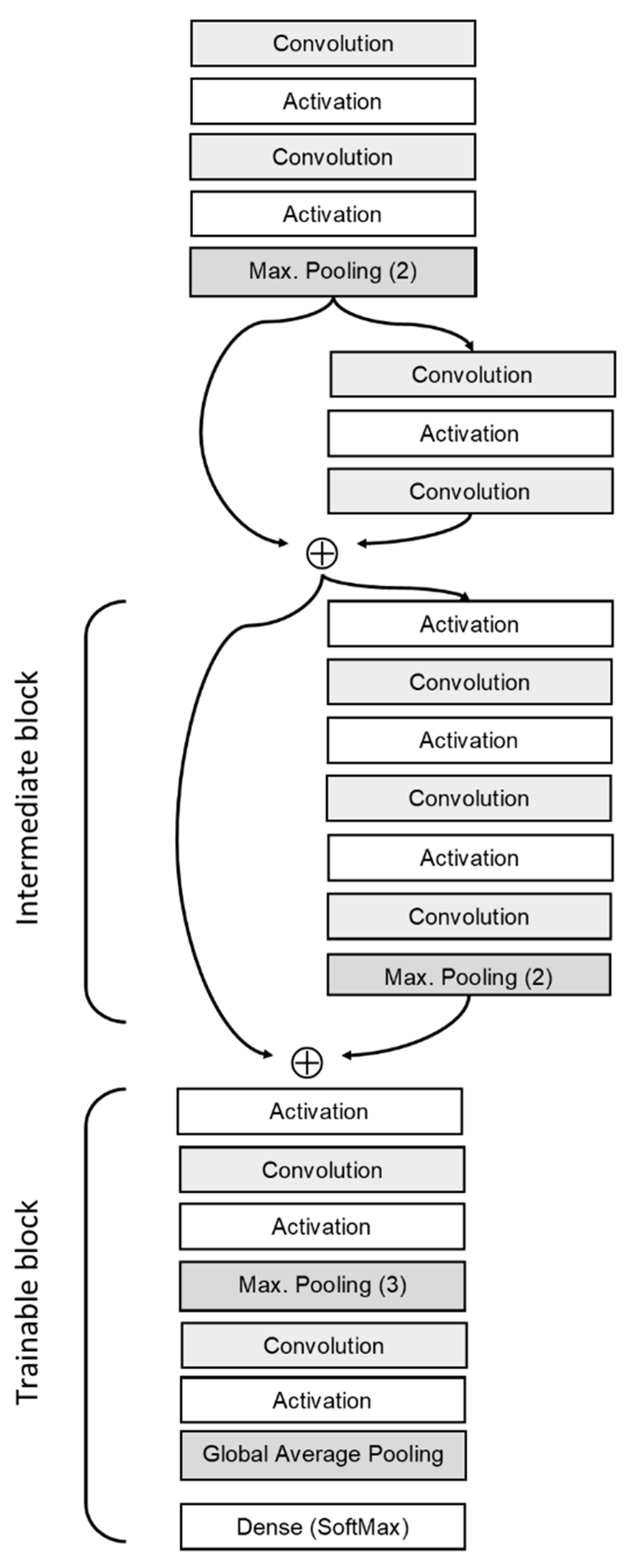
 Number of intermediate blocksChoice0, 1, 2, 321
 Top-layer configurationChoiceA: Global Average Pooling + Dense (Softmax)AA
B: Flatten + Dense + Dropout + Dense (Softmax)
Weight initialization
ChoiceA: Glorot (Xavier) normal initializerAA
B: He normal initializer
Activation
ChoiceReLUSwishSwish
LeakyReLU
PReLU
Trainable Swish
Regularization
 L2 lambdaLog-uniform10−7 to 10−31.33 × 10−51.01 × 10−7
Optimization
 Initial learning rateLog-uniform0.0002 to 0.0040.000680.00111
Table 2. Classification performance. Correct classification rate (accuracy) of the best standard convolutional neural networks (CNNs) and the best separable CNNs (sepCNNs) in ten trials.
30 Subjects36 Subjects (Transfer Learning)
TrialCNNsepCNNCNNsepCNN
10.9981.0001.0001.000
21.0001.0000.9991.000
30.9760.9980.9990.999
41.0000.9990.9991.000
50.9980.9990.9990.999
60.9990.9980.9990.999
70.9980.9030.9990.999
80.9990.9990.9990.999
90.9991.0000.9990.999
100.9980.9980.9990.999
Median99.84%99.89%99.91%99.93%
First quartile99.82%99.82%99.88%99.93%
Third quartile99.87%99.94%99.93%99.96%
Table 3. Results of the verification experiments. The ability of the best CNN to differentiate between authorized users and unauthorized users was evaluated in 4 × 25 trials. The 36 subjects were randomly assigned as authorized/unauthorized users for each trial, with four different proportions.
Authorized UsersUnauthorized UsersAUC (Median)AUC (1st Quartile)AUC (3rd Quartile)EER (Median)EER (1st Quartile)EER (3rd Quartile)
10260.999970.999940.999990.27%0.23%0.31%
15210.999970.999940.999980.25%0.19%0.33%
20160.999950.999910.999960.33%0.25%0.41%
25110.999960.999950.999990.32%0.23%0.39%
Average 0.99997 0.29%
AUC: area under the (receiver operating characteristic) curve. EER: equal error rate.
Table 4. Summary of representative studies in footstep recognition.
StudySubj.StepsFootwearFeatureClassifierPerformance
Jung et al. 2004 [17]11440BarefootFoot shape + COP trajectoryHMMFRR: 1.36%FAR: 0.14%
Suutala et al. 2007 [18]11440ShodVertical GRF profileSVM, MLPACC: 95%
Moustadikis et al. 2008 [15]402800Shod3D GRF profileSVMACC: 98.2%
Pataky et al. 2011 [16]1041040BarefootPlantar pressure patternKNNACC: 99.6%
Derlatka 2013 [14]1422500Shod3D GRF profileKNNACC: 98%
Connor 2015 [23]923000Barefoot and ShodMixedKNNACC: 99.8% (Barefoot)
ACC: 99.5% (Shod)
This study, identification36108,000ShodCOP trajectoryCNNACC: 99.9%
This study, verification36108,000ShodCOP trajectoryCNNEER: 0.3%
ACC: accuracy (correct classification rate). CNN: convolutional neural network. COP: center of pressure. EER: equal error rate. FAR: false acceptance rate. FRR: false rejection rate. GRF: ground reaction force. HMM: hidden Markov model. KNN: k-nearest neighbors. MLP: multilayer perceptron. SVM: support vector machine.

