1. Introduction
Hyperbolic topologies have sparked the imaginations of science fiction prosaists for almost a century [
1]. In turn, the topology of isofrequency k-surfaces in photonic materials now fascinates the members of the optics community. The known topologies include bounded k-surfaces, such as spheres or ellipsoids, and unbounded k-surfaces—single- and double-leaf hyperboloids [
2,
3,
4], and recently discovered bihyperboloids [
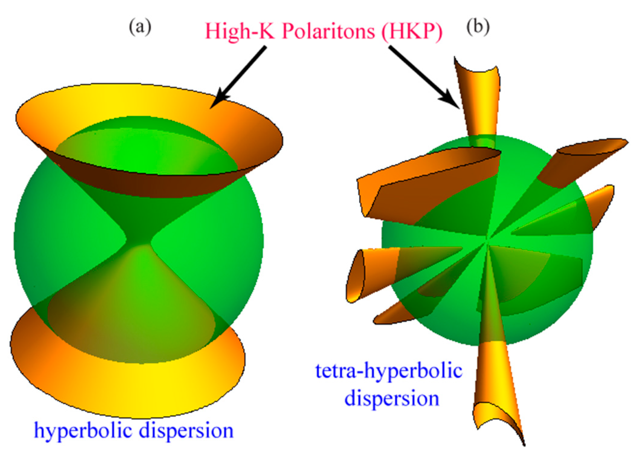
5]. As can be seen from this list of k-surface topologies, the main difference between them and therefore the key to their classification is the propagation or absence of high-k modes in the corresponding materials (
Figure 1). The high-k modes, which are the short-wavelength solutions of macroscopic Maxwell’s equations in hyperbolic metamaterials, are of primary interest in photonics, and have already found applications for optical imaging in nanoscopic resolution using hyperlenses, emission control due to diverging optical density of high-k states, and emission-directivity control [
6].
With the development of nanofabrication, a variety of bianisotropic and chiral metamaterials have been realized, which includes a combination of split-ring resonators, helixes, gammadions, and other metallic shapes in unit cells [
6]. In this letter we theoretically predict novel isofrequency topology phases, tri- and tetrahyperbolic materials, and obtain an equation that describes the k-space directions in which the high-k modes exist in terms of the 36 material parameters of an arbitrary bianisotropic material. Furthermore, we employ a theorem from Zeuthen (1873) [
7] to show that our prediction of the tri- and tetrahyperbolic topological phases completes the classification of bianisotropic materials, meaning that an optical material belongs to one of the following classes—tetra-, tri-, bi-, mono-, or nonhyperbolic. The novel tetra- and trihyperbolic phases which we predict here are induced via the introduction of chirality. Chirality-induced modification of topology in the energy–momentum space was previously studied for monohyperbolic materials [
8]. Here we discuss the topology of isofrequency surfaces in k-space.
We show that in all high-k modes, both electric and magnetic fields are polarized longitudinally. In this sense, these modes are similar [
9] to the bulk plasmon polaritons, bulk magnon polaritons, or longitudinal optical phonon polaritons, except that the high-k modes are short-wavelength. Therefore, we shall refer to these modes as high-k polaritons (HKPs). For these HKPs, we explicitly express the ratio between the longitudinal electric and magnetic field, i.e., longitudinal impedance
, in term of the 36 bianisotropic material parameters. To accomplish this, we introduce the index of refraction operator
. We obtain the direction-dependent refraction indices explicitly in arbitrary bianisotropic material.
2. Theory of Isofrequency Surfaces in Bianisotropic Materials
Consider bianisotropic materials with 6 × 6 effective parameters matrix
, such that the constitutive relations are given by
. It is known that the isofrequency surface of the most generic bianisotropic material with arbitrary material parameters
is a quartic surface in k-space given by [
10].
As was demonstrated in Ref. [
10], the coefficients
follow from the solution of Maxwell’s equation. The topological asymptotic skeleton of the isofrequency surfaces (Equation (1)) can be found in the high-k limit
. The high-k states are those tending to the conical k-surfaces given by
Below we establish the detailed form and properties of the function in terms of the material parameters and the topological properties of the skeleton asymptotic surfaces of Equation (2).
We start by considering Maxwell’s equations for the amplitudes
of the plane waves with wave vectors
and frequencies
written as
Consider a wave propagating in the direction
. Let us use the transformation
:
where
and vectors
are the rows of matrix
. Note that
and is a proper rotation
.
Let us apply transformation
to Maxwell’s Equation (Equation (3))
According to Equation (5) the transformed matrices
can be expressed in terms of the original
as
The zeroes in the bottom row of matrix
are due to the conditions
and
. Thus, the longitudinal components of fields
and
can be decoupled from the transverse field components in the transformed coordinates as
while the transverse components satisfy the system of equations
We rearrange this and introduce the index of refraction operator
:
The characteristic equation for the eigenvalue problem (Equation (9)) is a quartic equation equivalent to Equation (1), which is valid for a generic bianisotropic medium without an assumption of reciprocity
where
Consider reciprocal materials. The material parameters are bound by
, which is true in the transformed coordinates for the elements of
and for the elements of
in Equations (8) and (9). In this case
, which turns Equation (10) into
The roots of Equation (11) are
This is an explicit expression for the refraction indices of waves in arbitrary reciprocal materials, and this confirms our previous conclusion from Reference [
11], that isofrequency k-surfaces have reflection symmetry in reciprocal materials.
3. Results
Let us turn to the asymptotic behavior at high k. If one of the eigenvalues of the index of refraction operator
becomes infinite, then
also diverges, since it is the product of all the eigenvalues
. If the elements of the matrix
are finite, then, according to the expression for matrix
(Equation (8)), whose elements compose
(Equation (9)), such divergence is only possible for waves propagating in directions
such that
Considering Equation (6) and that
, Equation (13) can be rewritten as an equation of a quartic conical surface
where
for a generic bianisotropic medium without an assumption of reciprocity.
Direct comparison shows that function of Equation (14) is identical to Equation (2). Note that functions , where , are quadratic forms on k-space.
If
, then the longitudinal components of fields
and
are much greater than the transverse components, so
. Consequently, Maxwell’s equations can be written as
Equations (15) and (16) have a nonzero solution for the longitudinal fields only if Equation (14) is met. Note that from and , it follows that for HKPs , since HKP fields are purely longitudinal .
An important characteristic of an HKP is its longitudinal impedance, which we introduce using Equations (15) and (16):
For reciprocal materials,
and Equation (14) breaks into two solution branches:
corresponding to impedances
The conventional condition of hyperbolicity requires the principle values of the dielectric permittivity tensor
to be of different signs [
2,
3,
4]. Indeed, for such materials,
can only be zero if principle values of
have different signs. According to Equations (17) and (19), the longitudinal impedance for the HKP in these materials is
. Similarly, for magnetic hyperbolic materials [
12], the function from Equation (17) is
, assuming
is a scalar, and the tensor
has to have principle values of different signs. The HKP waves have
in magnetic hyperbolic materials (see Equations (17) and (19)).
It has been theoretically predicted in Reference [
7] that in the absence of magnetoelectric coupling (
, if both
and
have principal values of different signs at the same frequency
, then bihyperboloid isofrequency k-surfaces are possible. As can be seen from Equation (14), if
, then
and, indeed, two hyperboloids in the k-surface can form corresponding to electric
branch with
and magnetic branch
with
(cf. the discussion of Figure 3).
Let us consider anisotropic magnetoelectric coupling and study the drastic changes to the topology of the isofrequency surfaces it leads to. We first study materials which are nonhyperbolic in the absence of magnetoelectric coupling, i.e., the principal values of their and tensors have the same signs.
Consider a material with
,
, and
. Equation (14) then turns into
, which shows that HKPs propagate if
and
have opposite signs. Note that
does not lead to the formation of HKPs, since in this case a 0/0 indeterminacy forms in Equation (9), which resolves as 0, since for an isotropic chiral material
[
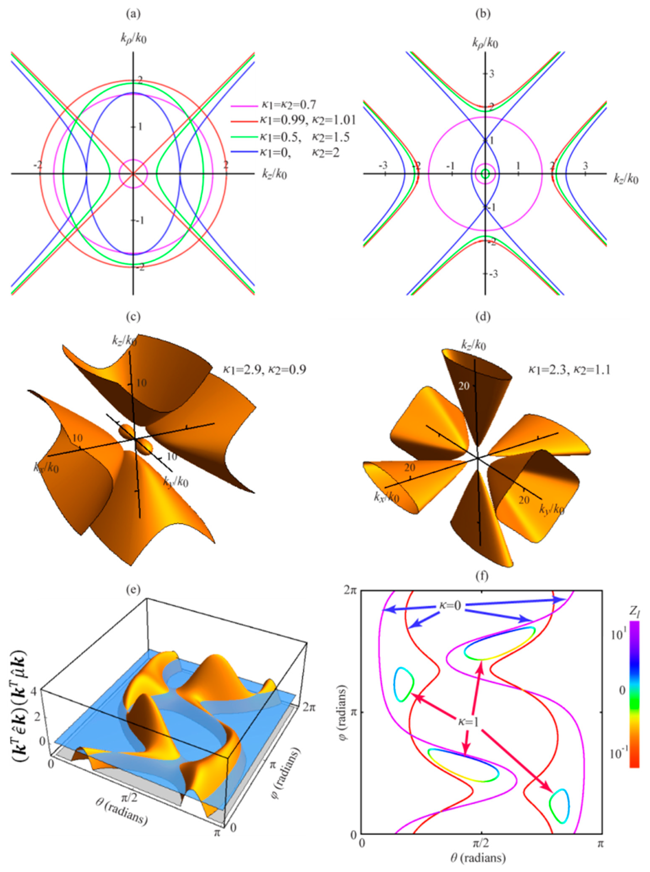
13]. The formation of a hyperbolic material here is due to the anisotropic chirality tensor and is shown in
Figure 2a.
If reciprocity is broken
, then
and a bihyperboloidal k-surface may form. In
Figure 2b we plot k-surfaces for a material with
,
, and
for the same values of
and
as in
Figure 2a and demonstrate the bihyperbolic dispersion.
In
Figure 2c,d we demonstrate that a material with anisotropic
,
, which is nonhyperbolic without magnetoelectric coupling, forms bihyperbolic and trihyperbolic phases if anisotropic chirality
is added with
and
for
Figure 2c and
and
for
Figure 2d.
Now let us turn to materials that are hyperbolic in the absence of magnetoelectric coupling and consider how magnetoelectric coupling changes their topologies and HKPs. Below we consider a numerical example of matrix
shown in the inset
Figure 3d (to the left of the black line). This matrix
describes an anisotropic material with the dispersion transitional between hyperbolic and bihyperbolic. The HKP propagation directions for
are illustrated in
Figure 2e,f. In
Figure 2e we plot the function
(yellow), whose intersection with zero (blue) corresponds to the HKP propagation direction. These directions are also plotted in
Figure 2f for the electric branch
, with
(purple) and magnetic branch
with
(red), which corresponds to the color scale for
shown to the right. Let us turn to a material characterized by matrix
, where
is responsible for magnetoelectric coupling. The change in the HKP propagation directions with increasing
from zero corresponds to raising the level of the blue plane in
Figure 2e to level
, which confines the HKP states to the positive region
. The HKP propagation directions for
are shown in
Figure 2f with four disconnected curves, which corresponds to bihyperbolic dispersion. These connectivity curves are color-coded corresponding to
of the HKP states.
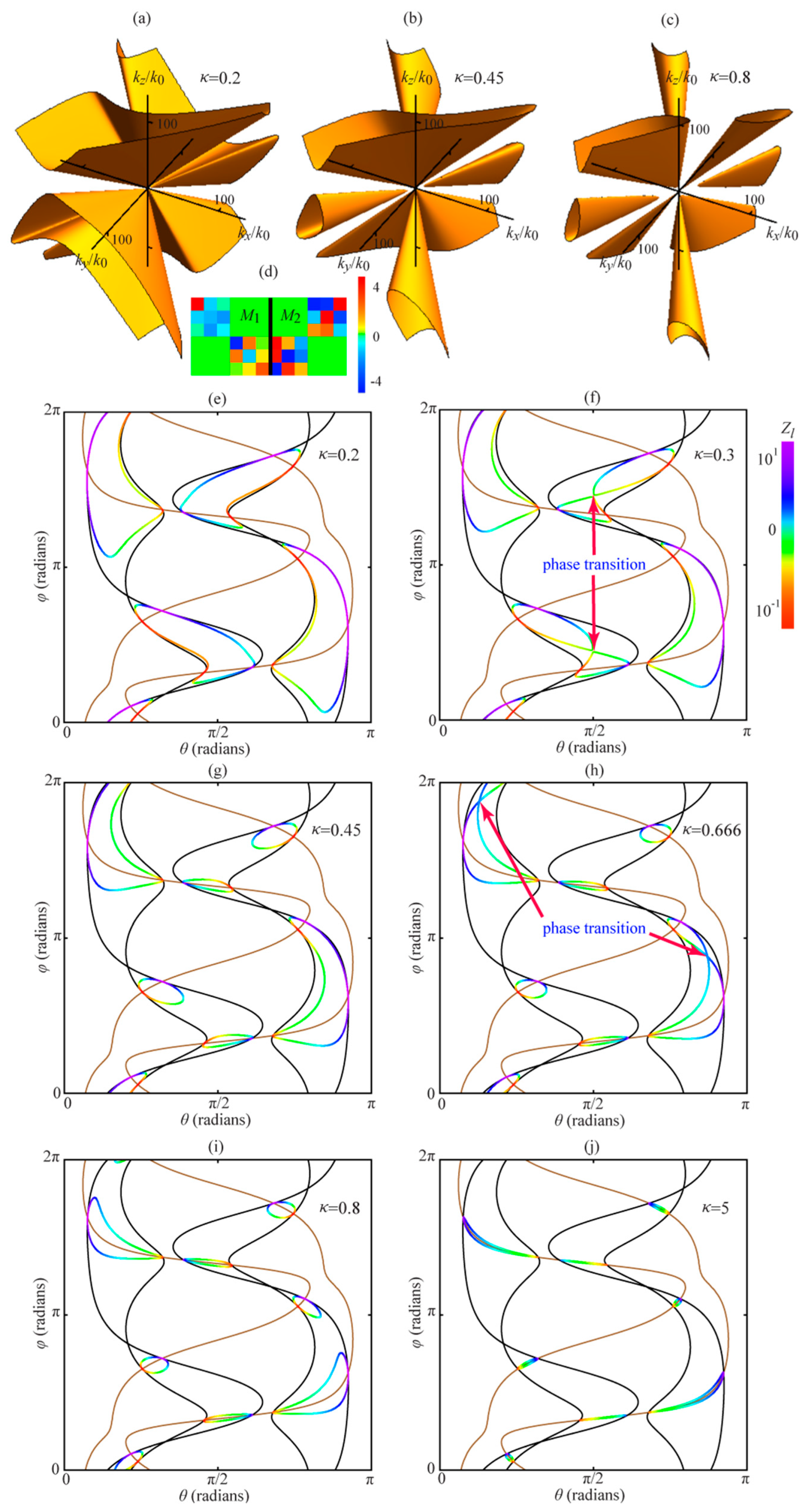
Let us consider a material described by the matrix
with the individual matrices
plotted on
Figure 3d. Changing parameter
leads to topological transitions between bihyperbolic (
Figure 3a,e), trihyperbolic (
Figure 3b,g), and tetrahyperbolic (
Figure 3c,i) phases. The progression of the phase changes is demonstrated in
Figure 3e–j. In these panels the HKP states for
satisfying
are outlined in black, which are the same curves as in
Figure 2f. The directions for which
and
(brown) satisfy Equations (14) and (18) for all
and serve as the framework for the topological transitions. These intersection points in
Figure 3e–j have invariant impedances
for the electric branch with
and
for the magnetic branch.
The HKP states for the
noted in panels (e)–(j) are color-coded in accordance with their
as indicated to the right of
Figure 3f. The HKP for nonzero
are positioned in the
regions between the
lines, in accordance with Equations (14) and (18), and touch these lines at the intersections of
and
. The HKP states group into several disconnected curves, the number of which characterizes the topology of the phase. Note that each curve is split into two parts by the
curves at their intersections with
. The resulting two subcurves of HKP states correspond to two different branches of Equation (18).
The addition of a small
leads to a transition to the bihyperbolic phase (four disconnected curves) as shown in
Figure 3e. At
(
Figure 3f), a phase transition occurs from the bihyperbolic to the trihyperbolic phase (six curves) in the k-space direction marked by the red arrows. In this direction the group velocity, which is normal to the k-surface, becomes zero
In general, we identify the condition (Equation (20) with topological phase transitions. The topological phase transition of the isofrequency k-surfaces were first discussed in Reference [
14] for the monohyperbolic phase. The transition from the trihyperbolic (
Figure 3g) to the tetrahyperbolic phase (eight curves in
Figure 3i) occurs at
(
Figure 3h). The k-space direction in which the transition occurs satisfies Equation (20) and is marked by the red arrows. For a large
, the HKP states closely follow the
curves between their intersections with
. Therefore, in the general case of arbitrary matrices
and
, the number of disconnected sections of
between their intersections with
can serve as the prediction of the topological phase of the isofrequency surfaces for a large
.


