Article

Image Registration Algorithm Based on Convolutional Neural Network and Local Homography Transformation

Faculty of Information Science and Engineering, Ningbo University, Ningbo 315211, China
*
Author to whom correspondence should be addressed.
Appl. Sci. 2020, 10(3), 732; https://doi.org/10.3390/app10030732
Submission received: 18 December 2019 / Revised: 15 January 2020 / Accepted: 16 January 2020 / Published: 21 January 2020
(This article belongs to the Special Issue Advances in Image Processing, Analysis and Recognition Technology)

Abstract

:
In order to overcome the poor robustness of traditional image registration algorithms in illuminating and solving the problem of low accuracy of a learning-based image homography matrix estimation algorithm, an image registration algorithm based on convolutional neural network (CNN) and local homography transformation is proposed. Firstly, to ensure the diversity of samples, a sample and label generation method based on moving direct linear transformation (MDLT) is designed. The generated samples and labels can effectively reflect the local characteristics of images and are suitable for training the CNN model with which multiple pairs of local matching points between two images to be registered can be calculated. Then, the local homography matrices between the two images are estimated by using the MDLT and finally the image registration can be realized. The experimental results show that the proposed image registration algorithm achieves higher accuracy than other commonly used algorithms such as the SIFT, ORB, ECC, and APAP algorithms, as well as another two learning-based algorithms, and it has good robustness for different types of illumination imaging.

1. Introduction

Image registration is a process of image matching and transformation of two or more different images. It is widely used in such fields as panoramic image splicing [1,2], high dynamic range imaging [3], simultaneous localization and mapping (SLAM) [4], and so on.
Traditional image registration algorithms are mainly classified into pixel-based algorithms and feature-based algorithms [5,6]. In pixel-based image registration algorithms, the original pixel values are directly used to estimate the transformation relationship between images [7,8]. Firstly, the homography matrix between a pair of images is initialized. Then, the homography matrix is used to transform the image, and the errors of pixel values of the transformed image are calculated. Finally, the optimization technique is used to minimize the error function to achieve image registration. The pixel-based algorithms usually run slowly and are effective to low-texture scenes, but have poor robustness to scale, rotation and brightness.
In feature-based image registration algorithms [9,10] such as SIFT [11], ORB [12], etc., feature points of images are generally extracted first, and the corresponding relationship between feature points of the two images is established by feature matching, and the optimal homography matrix is estimated by algorithms such as RANSAC [13], etc. Feature-based image registration algorithms are generally better and faster than pixel-based image registration, but feature-based algorithms require that there must be enough matching points between the two images and that the accuracy of matching points is higher and the location distribution of matching points is uniform. Otherwise, the registration accuracy will be greatly reduced. Feature-based image registration algorithms generally have good robustness to scale and rotation and have robustness to brightness to some extent, but are not suitable for low-texture images.
Recently, some deep learning-based image registration algorithms have been proposed. DeTone et al. [14] proposed a homography matrix estimation algorithm with supervised learning. A 128 × 128 image IA was generated by randomly clipping from an image I, and then random perturbation values were added to the coordinates of the four corners of the image IA to generate four perturbation points, so that four pairs of matching points were obtained. The homography matrix corresponding to the four pairs of points was calculated by using the coordinates of the four corners of image IA and their corresponding perturbation points. The homography matrix was used to transform image IA into image IB. Then, the images IA and IB were converted into grayscale images as samples, and the coordinate differences between the four corner points of IA and their corresponding perturbation points in IB were used as labels, with which a 10-layer VGG (Visual Geometry Group) network was trained, and finally a homography matrix estimation model that could be used for image registration was obtained. The algorithm has better robustness to brightness, scale, rotation, and texture. On the basis of DeTone’s work, Nguyen et al. [15] proposed a homography matrix estimation algorithm with unsupervised learning to solve the shortcoming of artificially generated labels in supervised learning, but this algorithm had weak robustness to illumination. The samples used in these two algorithms were mainly artificially generated samples. The artificial samples ensured that the accuracy of the samples and labels was high enough, which was a beneficial exploration for deep learning to solve the actual image registration problem. However, the artificial samples adopted by these two works default to no parallax between the images to be registered, so only four pairs of corresponding points are used to represent the registration relationship between the two images. However, in practice, there is parallax between the images to be registered, and the relationship between such kinds of images is often not exact homography transformation.
In image registration, it is necessary to estimate the homography matrix between the target image and the reference image. The homography matrix is used to transform the target image to achieve the alignment of the target image and the reference image in spatial coordinates. The transformation process is called image mapping or image transformation. According to the application scope of the homography matrix, image transformation can be divided into global homography transformation and local homography transformation. Global homography transformation [7,11,12,14,16] uses the same homography matrix to transform the whole image. It requires that the target image and the reference image contain basically the same image information in the overlapping region. It is only suitable for images with small or no parallax. When this condition is not satisfied, the accuracy of image registration will be reduced significantly. Local homography transformation algorithm [17,18,19] maps different regions of an image using different transformation matrices, which can better overcome the shortcomings of the global homography transformation algorithm. As-Projective-As-Possible (APAP) algorithm [19] is a representative local homography transformation algorithm. It first extracts the feature matching points between the images and then divides the images into a uniform grid. Moving direct linear transform (MDLT) is used to estimate the homography matrix of each grid. Finally, the homography matrix of each grid is used to implement local homography transformation on the image to be registered. For images that do not satisfy the condition of global homography transformation, the image registration accuracy achieved by APAP algorithm is higher than that achieved by the global homography transformation algorithm [20]. APAP algorithm is also a feature-based image registration algorithm in essence. It also has the characteristics of a feature-based image registration algorithm and has higher accuracy than the general feature-based image registration algorithm. The general image registration algorithm based on global homography transformation only uses one homography matrix estimation and one homography transformation, while APAP algorithm needs multiple homography matrix estimations and homography transformations, so the speed of the APAP algorithm is slower than that of the general feature-based image registration algorithm.
The above two deep learning-based image registration algorithms are both for global homography transformation, and the used samples cannot be adopted to estimate the local homography matrix. Therefore, based on the above researches, an image registration algorithm based on deep learning and local homography transformation is proposed in this paper. An image sample and label generation method suitable for local homography transformation is designed so as to train the image registration model with convolutional neural network (CNN) effectively. The resulted image registration model can effectively reduce the error of image registration and overcome the defects of poor robustness of traditional image registration algorithms and low accuracy of existing deep learning-based image registration algorithms.
The main contributions of this paper are as follows: (1) A CNN and local homography transformation-based algorithm are proposed to solve the problem of image registration, which is a useful exploration for deep learning to solve the problem of image registration; (2) an image sample and label generation method suitable for local homography transformation is proposed, and the generated samples have good diversity and can simulate the actual image registration situation.
The rest of this paper is organized as follows. Section 2 mainly introduces the basic theory of the proposed algorithm, focusing on the image sample, label generation, CNN model, and loss function. Section 3 shows the experimental results, which verify the effectiveness of the proposed algorithm. The conclusion is given in Section 4, which summarizes the main work of this paper and analyses the shortcomings of the algorithm and possible improvement aspects.

2. Image Registration Algorithm Based on Deep Learning and Local Homography Transformation

In supervised learning-based image registration, sample labeling is required first. However, the cost of labeling samples manually is too high, and it is usually difficult to ensure the labeling accuracy, as well as to collect enough diverse images for registration. To solve this problem, an image registration algorithm based on deep learning and local homography transformation is proposed in this paper. Firstly, a sample and label generation method for deep learning is designed. In this method, direct linear transformation (DLT) and moving direct linear transformation (MDLT) are used to automatically generate more reasonable and effective samples and labels for deep learning, and then supervised learning is used to train CNN so as to obtain the image registration model, with which the local homography transformation-based image registration can be achieved.

2.1. Direct Linear Transformation (DLT)

If there is no parallax between the reference and target images, the mapping relationship between the two images is simple homographic, which can be described by the homography matrix. Suppose that two points with coordinates x = [ x , y ] T and x = [ x , y ] T are the corresponding matching points on the reference image I’ and the target image I respectively, and the corresponding relationship between these two points can be expressed as
x ˜ = H x ˜
where x ˜ and x ˜ are the homogeneous coordinates of the two points respectively, and x ˜ = ( x y z ) , x ˜ = ( x y 1 ) , H is the homography matrix between the two images, H = ( h 11 h 12 h 13 h 21 h 22 h 23 h 31 h 32 h 33 ) .
In the non-homogeneous coordinates, the corresponding relationship between matching points x and x can be expressed as
x = x z = h 11 x + h 12 y + h 13 h 31 x + h 32 y + h 33 y = y z = h 21 x + h 22 y + h 23 h 31 x + h 32 y + h 33
Transform Equation (1) into the form of 0 3 × 1 = x ˜ × H x ˜ and obtain
( 0 0 0 ) = ( 0 0 0 x y 1 x y y y y x y 1 0 0 0 x x y x x x y y y y x x y x x 0 0 0 ) h
where h = ( h 11 h 12 h 13 h 21 h 22 h 23 h 31 h 32 h 33 ) T .
When estimating H, more matching point information can be used to reduce the estimation error. In Equation (3), only two rows of the 3 × 9 coefficient matrix on the right side of the equation are independent. By selecting the first two rows to form an independent coefficient matrix A i , and taking all matching points into account, a 2N × 9 coefficient matrix A can be formed. By using the least square method, the solution of h can be expressed as
h ^ = arg min h i = 1 N A i h 2 = arg min h A h 2
where h ^ is an estimation of h, A h denotes the two norms of vector Ah, h is the normalized unit vector, N denotes the total number of pairs of matching points, and A i denotes the independent coefficient matrix corresponding to the ith pair of matching points. Singular value decomposition (SVD) can be used to calculate h ^ . The right singular vector corresponding to the minimum singular value of A is the result. The estimation of homography matrix H is obtained by arranging the elements of vector h ^ in a certain order.
Considering that SVD is time-consuming, which will affect the training speed of the neural network, Equation (3) is transformed into the form of non-homogeneous linear least squares. Let h 33 = 1 , two independent non-homogeneous linear equations can be obtained as
A i h = b i
A i = ( 0 x 0 y 0 1 x 0 y 0 1 0 x y y y x x y x )
h = ( h 11 h 12 h 13 h 21 h 22 h 23 h 31 h 32 ) T
b i = ( y x )
If all N matching points are included, then Equation (4) can be represented as
h ^ = arg min h i = 1 N A i h b i 2 = arg min h A h b 2
where h ^ is the estimation of h , and A is the coefficient matrix of 2N × 8 obtained by arranging all coefficient matrices A i in the vertical direction. b is a constant column matrix of 2N × 1 obtained by arranging all the constant column matrices b i in the vertical direction.
Let E = A h - b 2 ; h ^ can be calculated through d E d h = 0
h ^ = ( A T A ) 1 A T b

2.2. Moving Direct Linear Transformation (MDLT)

For an image with a certain parallax, the relationship between the reference and target images is no longer a simple homography transformation. In this case, the global homography transformation cannot ensure the accuracy of image registration, and simple local homography transformation will cause a blocking effect, which destroys the visual quality of the image. It is a good choice to use the MDLT algorithm for local homography transformation. The MDLT algorithm not only has high accuracy of image registration, but also can smooth different image blocks, taking into account the accuracy of image registration and the overall visual quality of the image.
Firstly, the image to be transformed is divided into several image blocks, and then all matching points of the two images are taken into account. For each of the image blocks, according to the central position of the image block, the weights are assigned to all matching points so as to estimate the homography matrix corresponding to this image block. Accordingly, Equation (4) can be rewritten as
h ^ j = arg min h j i = 1 N ω i j ( A i h b ) 2 = arg min h j W j ( A h - b ) 2
where h ^ j represents an estimation of the homography matrix of the jth image block, ω i j is a weight that changes with the coordinate of the center point of the current image block, and W j is a diagonal matrix that represents the weights of all matching points, and
W j = diag ( [ ω 1 j ω 1 j ω i j ω i j ω N j ω N j ] )
The weight ω i j is determined by the distance between the ith matching point and the center point of the jth image block. The smaller the distance, the larger the weight. Zaragoza et al. [19] used Gaussian function to calculate the weight
ω i j = max ( exp ( x i x j 2 σ 2 ) , γ )
where x j represents the coordinate of the center point of the jth image block, x i represents the coordinate of the ith matching point of the image to be transformed, σ is the scale factor, and γ is the minimum weight value, which prevents the weight of some matching points far from the current image block from being too small.
Lin et al. [21] proposed another method of calculating weights, using Student-t distribution function instead of Gaussian distribution function, which is represented as
ω i j = ( 1 + x i x j 2 ν σ 2 ) ν + 1 2
Because the student t-distribution function is smoother than the Gaussian distribution function, it is not easy for the block effect caused by local homography transformation to appear, so the student-t distribution function is adopted in this paper. By using the same analysis method of the DLT algorithm, the estimation of the local homography matrix is finally calculated as follows:
h ^ j = ( A T W j 2 A ) 1 A T W j 2 b

2.3. Sample and Label Generation Method Based on Local Homography Transformation

In the homography matrix, the rotational and shear components are often much smaller than the translation components, so it is difficult for a model to converge if the homography matrix is used as a label directly. Therefore, DeTone et al. proposed a method of substituting four pairs of corresponding points for the homography matrix [14]. The algorithm uses global homography transformation and is only suitable for the registration of an image without parallax. However, the actual images usually have parallax.
To overcome the shortcomings of DeTone’s method, an improved sample generation method based on local homography transformation is proposed to generate sample images with parallax, as illustrated in Figure 1. The sample and label generation process is described in detail as follows:
Step 1: Firstly, add random perturbation values to the coordinates of the four corners {P1, P2, P3, P4} of the original image IA to obtain four new points {P′1, P′2, P′3, P′4}, where the ranges of the random perturbation values in horizontal and vertical directions are [−ρx, ρx] and [−ρy, ρy], respectively. The two points before and after the perturbation form a pair of corresponding points, therefore, a total of four pairs of corresponding points are obtained, as shown in Figure 1a. Then, calculate the homography matrix H 4 p t A B corresponding to the four pairs of corresponding points.
Step 2: Randomly select a point p in the original image IA, cut out a block I A with fixed size using pas the upper left corner of the block, and divide the block into a uniform grid to get M × N grid points GA, as illustrated in Figure 1b.
Step 3: According to Equations (1) and (2), transform the M × N grid points GA into new corresponding M × N points G A by using the homography matrix H 4 p t A B , as illustrated in Figure 1c.
Step 4: Add random perturbation values to each of the new corresponding M × N points G A to get M × N perturbation points G ˜ A , as illustrated in Figure 1d. The ranges of random perturbation values in horizontal and vertical directions are [ ρ x , ρ x ] and [ ρ y , ρ y ] , respectively, and ρ x < ρ x / 2 , ρ y < ρ y / 2 , so as to ensure the global consistency of these random perturbation points.
Step 5: Through the M × N uniform grid points, GA generated in Step 2 and M × N corresponding perturbation points G ˜ A generated in Step 4, the corresponding global homography matrix H g A B is calculated by the DLT algorithm. Then transform the M × N uniform grid points GA into new points G A by using H g A B and calculate the root mean square error (RMSE) between G ˜ A and G A . After that, divide the original image IA into an m × n uniform grid according to the RMSE, as shown in Figure 1e. If the RMSE is large, which means that there is a strong locality between GA and G ˜ A , the grid of the original image should be partitioned smaller to improve the local accuracy; conversely, if the RMSE is small, it means that the local homography matrixes have strong global character, therefore, the grid of the original image can be partitioned larger so as to speed up sample generation. The number of rows and columns of the uniform grid can be determined by
m = int ( min ( 1 + H y r m s e ρ y h min , H h min ) ) , n = int ( min ( 1 + W x r m s e ρ x w min , W w min ) )
where m and n are the number of rows and columns of the uniform grid, W and H are the width and height of the image IA, xrmse and yrmse represent the RMSE between G ˜ A and G A in horizontal and vertical directions, and wmin and hmin represent the minimum width and minimum height of each image block, respectively. wmin and hmin should not be too small, otherwise, it will cause too many blocks of some samples, which will affect the speed of sample generation; however, it also should not be too large, so as to avoid too few blocks of samples, which will result in an unnatural block effect in the transformed image.
Step 6: Calculate the local homography matrix H j A B ( j = 1 , 2 , , m × n ) corresponding to each block of the m × n uniform grid with the MDLT algorithm, in which the M × N pairs of corresponding points between GA and G ˜ A are used as the pairs of matching points, so that the m × n local homography matrixes H L A B = { H j A B | j = 1 , 2 , , m × n } are obtained. Then transform the original image IA into a new image IB with H L A B and calculate the coordinate of the points GB in image IB corresponding to GA in IA with H L A B .
Figure 1f shows the image IB generated from the original image IA shown in Figure 1a after local homography transformation, and the grid points in Figure 1f represent the new grid points generated by local homography transformation corresponding to the M × N uniform grid points GA in Figure 1b.
Step 7: For image IB, an image block with the same size and coordinates as that of I A in image IA is cropped as I B . Image I A and image I B constitute the alternative sample of the neural network. The coordinate difference GAB between the points GB in image IB and its corresponding points GA in image IA forms the alternative label of the neural network.
Figure 1g gives a pair of alternative samples cropped from the images in Figure 1b,f.
Step 8: In the process of generation of image IB, if the overlap degree of two sample images is too low because of the extreme distribution of perturbation point G ˜ A , the samples are regarded to be invalid and will be discarded.
The calculation of the overlap degree of two sample images is illustrated in Figure 1h. Let I A be the corresponding binary mask of sample image I A in the original image IA. Transform the mask image I A through the local homography matrix H L A B so as to obtain the corresponding binary mask I B in the image IB. Then the binary mask images I A and I B are intersected to get the binary mask image I A B , in which the non-zero-pixel region indicates the overlap region of the two sample images, as shown in Figure 1h. Thus, the overlap degree of two sample images is calculated as
= S A B S A
where denotes the overlap degree, SA denotes the number of non-zero pixels in I A , and SAB denotes the number of non-zero pixels in I A B . If of two sample images is lower than a threshold, the two sample images will be discarded.

2.4. Loss Function and Convolutional Neural Network

RMSE can be used as a loss function of CNN, which is defined by
L s = 1 k i = 1 k x i x ^ i 2
where xi is the label value of the ith pair of matching points, x ^ i is the corresponding output value of the CNN, and k is the total number of pairs of matching points.
General CNN can be used to obtain the image registration model. In this paper, three network architectures including VGG [22], Googlenet [23] and Xception [24] are compared. The structure of the VGG network is simple and the depth of the network is easily expanded, but its training speed is slow and it requires a lot of hardware resources. For simplicity, we adopted a 10-layer VGG network [14] in the experiments. Googlenet can deepen the depth and width of the neural network, speed up the training speed, and reduce the hardware resources needed by the network. The convergence speed of the Xception network is fast, and the hardware resources required are also less. Additionally, the convergence performance of the Xception network is generally better than that of VGG and Googlenet networks.

3. Experimental Results and Analysis

To test the performance of the proposed algorithm, it is compared with Scale-Invariant Feature Transform (SIFT) algorithm [11], Oriented FAST and Rotated BRIEF(ORB) algorithm [12], Error Checking and Correction (ECC) algorithm [7], APAP [19], the DeTone’s algorithm [14], and the Nguyen’s algorithm [15]. The experiments are implemented on a computer with Intel i7-6700 CPU, 32 GB memory, one NVIDIA GTX 1080 Ti GPU, and the operating system used is Ubuntu 16.04 LTS.
The performances of different image registration algorithms are compared in terms of accuracy, running time and robustness. The three algorithms of SIFT, ORB and ECC are implemented by using Python OpenCV. The RANdom SAmple Consensus (RANSAC) threshold of SIFT and ORB algorithms is 5. The maximum number of iterations of the ECC algorithm is 1000. The adopted framework of deep learning is TensorFlow [25]. The APAP, DeTone’s algorithm and Nguyen’s algorithm are implemented with Python programming language on the same platform.
To facilitate comparison with the DeTone’s and Nguyen’s algorithms, the size of sample images used in this paper is the same as that of DeTone’s and Nguyen’s algorithms. The used perturbation values consist of components in horizontal and vertical directions, the range of which should not be too small or too large. If the perturbation range is too small, the generated perturbation value will be small, which will reduce the diversity of the samples and weaken the generalization ability of the model. However, if the perturbation range is too large, it may easily generate some samples with extreme deformation, which will make the training of the model more difficult and lead to the reduction of prediction accuracy of the model. The maximum perturbation values ρx or ρy of corner points in Step 1 of the proposed image sample and label generation method should not exceed half of the width or height of the original image respectively. Generally, taking 1/3~1/10 of the image width or height can ensure that the generated samples have better diversity and visual quality. Similarly, in Step 4, taking 1/3~1/10 of ρx for ρ x , 1/3~1/10 of ρy for ρ y can achieve better results.
The original data sets used in the experiments are MS-COCOCO2014 and MS-COCOCO2017 data sets [26]. Firstly, all images in these two data sets are scaled to 320 × 240, on which the proposed sample and label generation method is performed to obtain the gray-scale sample images with the size of 128 × 128. The maximum perturbation values ρx and ρy in horizontal and vertical directions of the corner points in Step 1 are set to 45, and the number of matching points for each pair of images in Step 2 is set to 5 × 5. The maximum perturbation values ρ x and ρ y in Step 4 are set to 11. In Step 5, the values of wmin and hmin are both 5. In Step 8, the threshold of overlap degree is 0.3, that is, when the overlap degree is lower than 0.3, the sample will be discarded. To increase the robustness of the model and reduce the possibility of over-fitting, image augmentation technology [27] is also used in the generation of training samples. The color and brightness of some of the sample images are randomly changed, and some of the sample images are processed with Gamma transformation. Finally, a total of 500,000 pairs of images are generated as a training set, 10,000 pairs of images as a validation set, and 5000 pairs of images as a test set.
In order to prove the generality of the proposed algorithm, three CNNs, including VGG, Googlenet and Xception, are used to train and test each of the learning-based image registration algorithms. The used optimization algorithm is Adam [28], where β 1 = 0.9 , β 2 = 0.999 , ε = 10 8 . The batch size is 128. The initial learning rate of the proposed algorithm and supervised learning of DeTone’s algorithm is 0.0005, and that of unsupervised learning of Nguyen’s algorithm is 0.0001. To prevent over-fitting, dropout [29] is used before the output layer of all neural networks. In the process of training, the test error of the validation set can be observed. When the test error of the validation set is no longer reduced, the training is stopped to prevent under-fitting or over-fitting.
When training the network models of the DeTone’s algorithm and Nguyen’s algorithm, the perturbation values of their samples are also set to 45, the same optimization techniques and image augmentation techniques as well as the same CNN are adopted. The number of training samples generated is the same as that of the proposed algorithm, and the training methods and observation methods are also the same. All algorithms are tested on the test set generated by the proposed method to ensure the objectivity of the comparison.

3.1. Accuracy of Image Registration

The accuracy of image registration can be measured by RMSE of registration points, which is defined by
R M S E ( f ) = 1 k i = 1 k f ( x i ) x i 2
where xi denotes the coordinates of grid points GA in image IA, and x i denotes the coordinates corresponding to xi in image IB; f represents different image registration models, and the proposed algorithm and APAP algorithm use the local homography matrix, while the other algorithms use the global homography matrix as their image registration model; f(xi) denotes the coordinates transformed from xi by using the image registration model f, which is the estimation of x i ; k is the total number of matching points in the pair of images, and it is set to 25 in the experiments.
Table 1 shows the average RMSE of registration points achieved by several different image registration algorithms when implemented on the test set generated by the proposed method. To better present the performance of learning-based image registration algorithms, Table 1 gives in detail the registration accuracy of several deep learning-based image registration algorithms using VGG, Googlenet and Xception neural networks, respectively.
From Table 1, it can be seen that the accuracy of the pixel-based ECC image registration algorithm is the lowest, and that of the feature-based SIFT image registration algorithm is higher. The APAP algorithm takes into account the locality of image registration, so it achieves the best result among the pixel-based and feature-based algorithms. The performance of the learning-based image registration algorithms is related to the used CNN models, and more advanced CNN models have higher image registration accuracy. The samples used by the DeTone’s algorithm and Nguyen’s algorithm are relatively simple, so there is little difference in the accuracy of image registration under different neural networks. These two algorithms do not fully consider the locality of image registration, resulting in low accuracy of image registration. Compared with other algorithms, the proposed algorithm achieves the highest image registration accuracy by using the Xception network model. In addition, from Table 1, it is seen that the effect of the proposed algorithm under Xception network is better than that under Googlenet and VGG networks. This is because the samples and labels used in the proposed algorithm are more complex, and there are obvious differences under different neural networks. When combined with more advanced CNN models, the proposed algorithm can achieve higher accuracy of image registration.

3.2. Running Time

To compare the calculation complexity of different image registration algorithms, Table 2 shows the average running time of each algorithm running for 10 times, where all algorithms are implemented under a computer with Intel i7-6700 CPU, 32 GB memory and one NVIDIA GTX 1080 Ti GPU. It is seen that APAP algorithm runs slowest due to the use of the local homography matrix and ORB algorithm runs fastest among the traditional image registration algorithms. For learning-based image registration algorithms, Table 2 gives the running time when the algorithms are accelerated with one GPU, as well as the running time achieved without the GPU. It is seen that GPU can significantly speed up the learning-based algorithms. The running speed of GPU is much faster than that of CPU, and different neural network models achieve different running speeds, among which Xception runs the slowest and Googlenet runs the fastest. Because the DeTone’s and Nguyen’s algorithms are only different in loss function and the neural network model is basically the same, the running time of the two algorithms are the same under the same conditions. The proposed algorithm involves the estimation of local homography matrices, so it runs slower than DeTone’s and Nguyen’s algorithms under the same neural network.

3.3. Robustness to Illumination, Color and Brightness

In order to compare the robustness of different image registration algorithms to illumination, color, and brightness, the test set in the experiments is augmented, and the used image augmentation method is the same as that of the training set. After image augmentation, the registration accuracy and failure rate of each algorithm are compared. We only randomly augmented some of the images in the test set, but not all of them. The higher the number of augmented images is, the higher the image augmentation degree of the test set is, and the test set has more diversity in illumination, color and brightness. The image augmentation degree can be represented by the probability of an image being augmented in the test set. The test set used in this experiment contains 5000 pairs of test images. Each algorithm runs 10 times repeatedly, during which the image augmentation is randomly implemented at a pre-specified image augmentation degree, and the average result of the 10 runs is taken as the final result of this algorithm with respect to the pre-specified image augmentation degree. Therefore, the image augmentation degree also represents the degree that the test set is affected by image augmentation.
The accuracy and failure rate of image registration can be used to measure the robustness of different image registration algorithms. Since the maximum perturbation values of each grid point in the sample image in the horizontal and vertical directions are ρx and ρy respectively, when the accuracy of image registration of a pair of images is greater than ρ 2 x + ρ 2 y , the pair can be considered as a registration failure, and the failure rate of image registration on the test set can further be calculated. Considering that the RMSE values of test samples failed to be registered may be too large, and these extreme data may affect the RMSE values of the whole test set greatly, therefore, the RMSE of the whole test set is defined as
R M S E i = min ( R M S E i , ρ 2 x + ρ 2 y ) R M S E = 1 K i = 1 K R M S E i
where RMSEi represents the RMSE value of the ith pair of images, and K denotes the total number of image pairs in the test set.
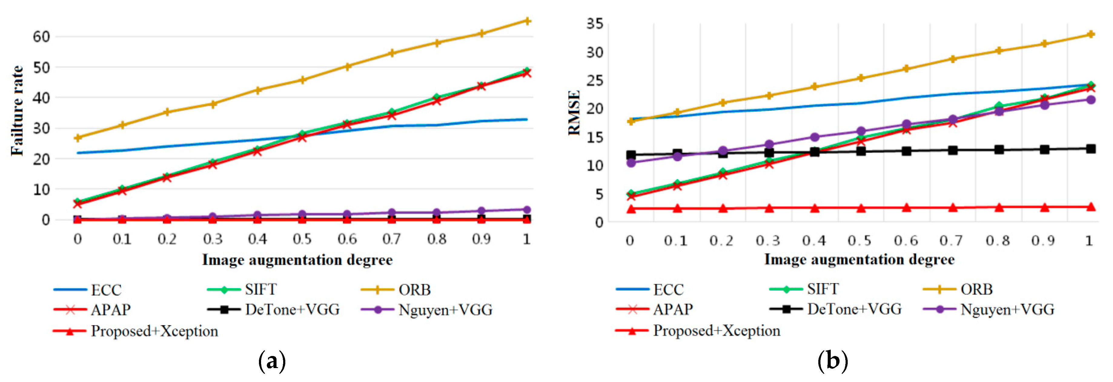
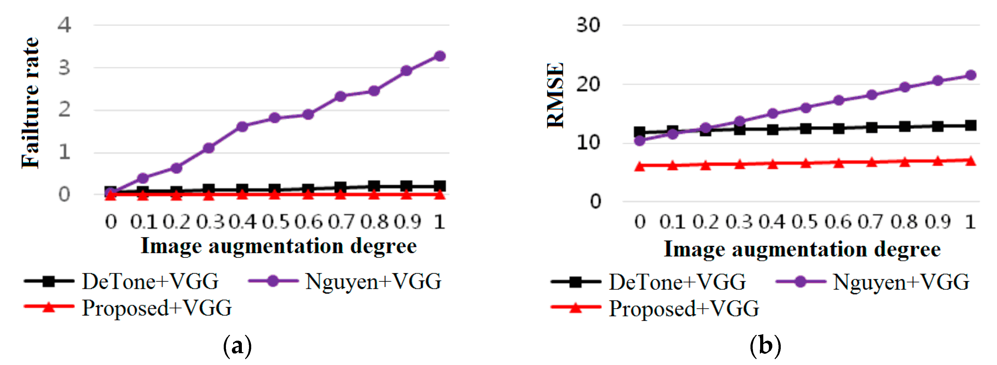
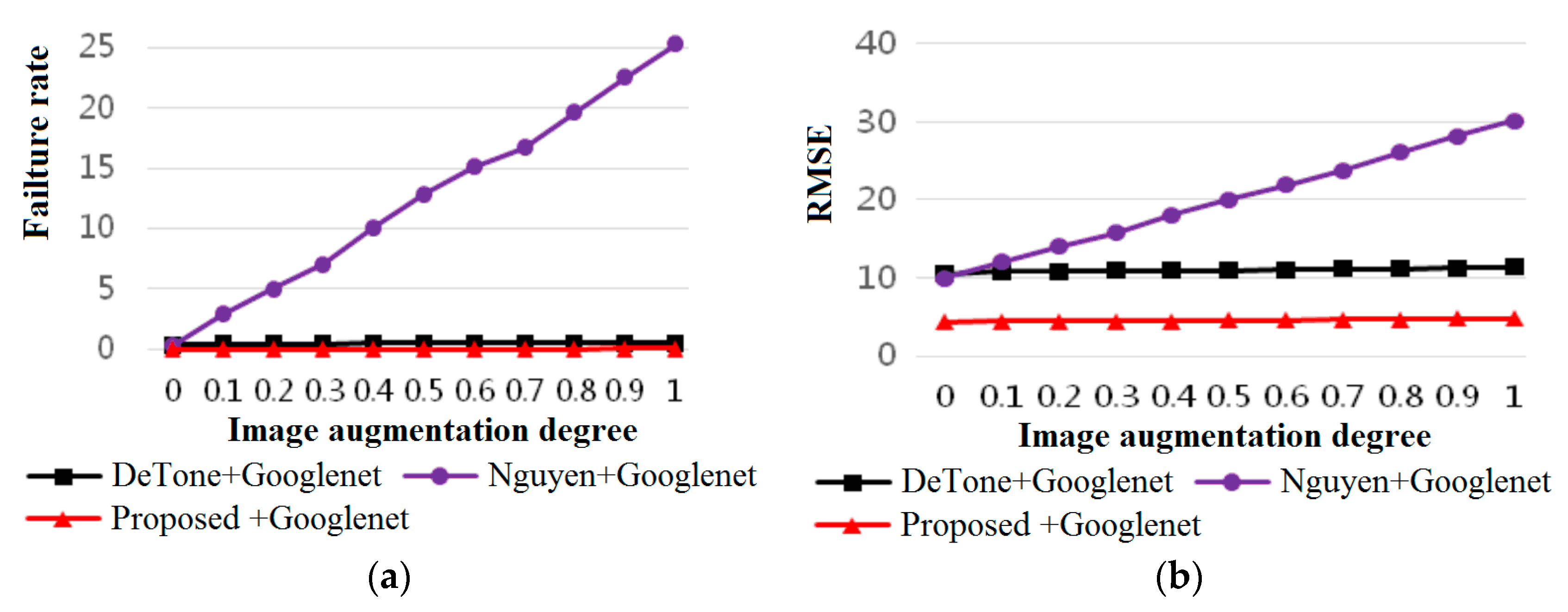
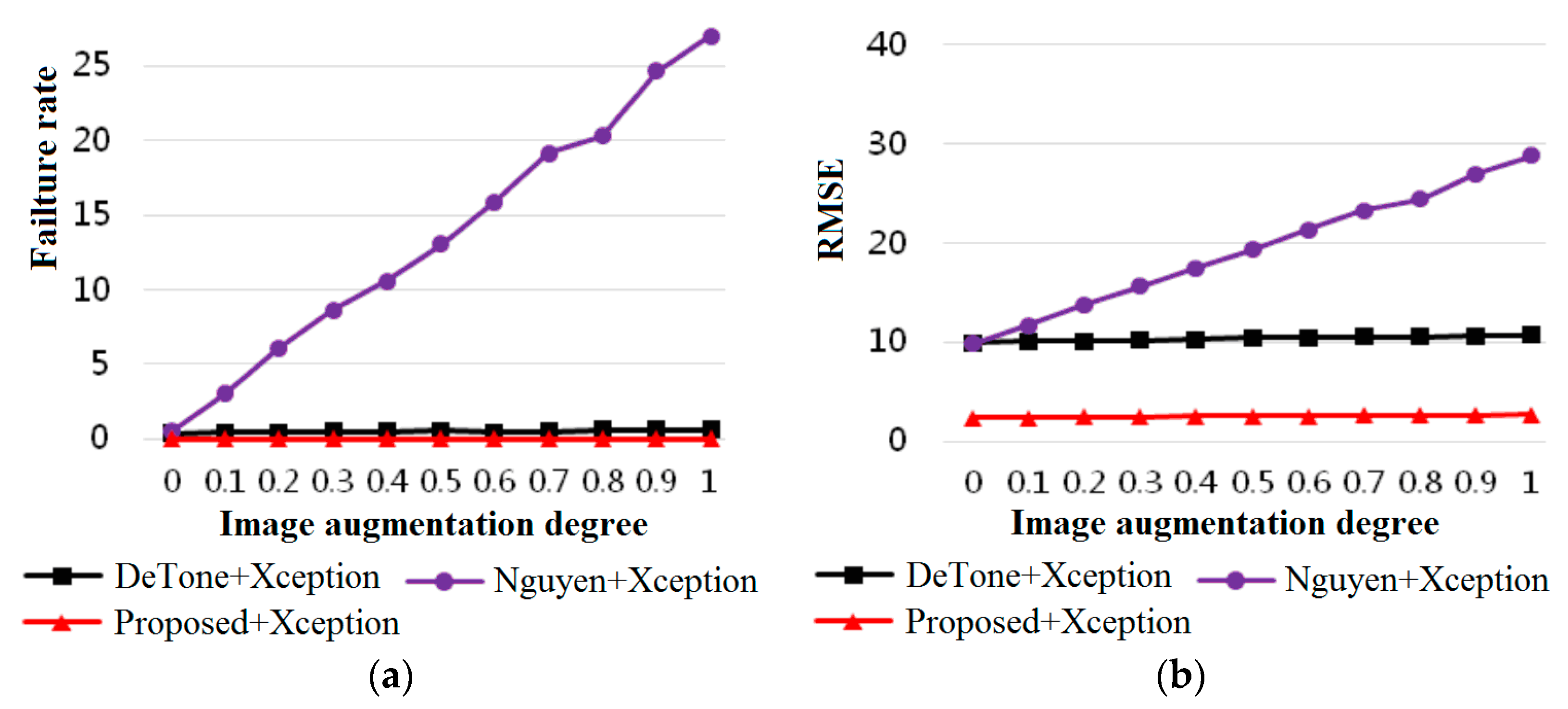
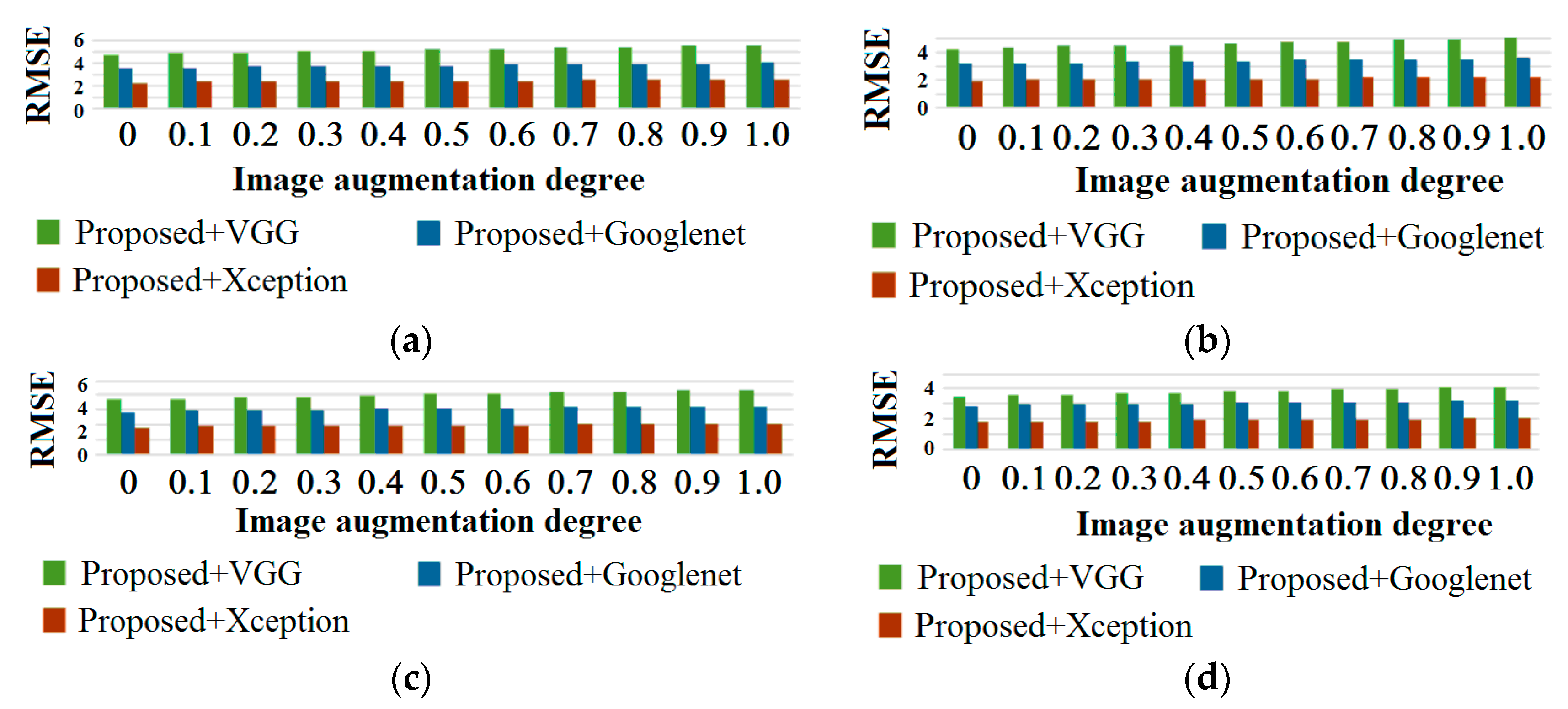
Figure 2, Figure 3, Figure 4 and Figure 5 show the failure rate and RMSE achieved by different algorithms under different image augmentation degrees. The abscissa is the image augmentation degree of the test set, which changes from 0.0 to 1.0 with a step size of 0.1; the ordinate represents the registration failure rate or RMSE. Figure 2 shows the robustness comparison of seven image registration algorithms, in which the CNN model used by DeTone’s and Nguyen’s algorithms is VGG, while the model used by the proposed algorithm is Xception. As can be seen from Figure 2, the robustness of the traditional image registration algorithms to illumination, color, and brightness is very poor, and the robustness of the learning-based algorithms, especially the supervised learning-based algorithm, is better than that of the traditional ones. Figure 3, Figure 4 and Figure 5 further give robustness analysis of the three learning-based image registration algorithms under three different CNN models. The used three CNN models are VGG, Googlenet and Xception, respectively. It can be seen that under the same neural network model, the robustness of Nguyen’s algorithm is inferior to the other two algorithms. Nguyen’s algorithm uses L1 norm as a loss function in the unsupervised learning algorithm, requiring the same image augmentation parameters for I A and I B in each pair of samples during the training, otherwise, the model will not converge normally, which results in the poor robustness of the unsupervised learning image registration algorithm. In contrast, DeTone’s algorithm and the proposed algorithm do not have this problem, because both of them adopt supervised learning; the label value can supervise the training of the neural network very well, so the model has better robustness.
In order to further analyze the influence of different perturbation values on the accuracy of the proposed algorithm, four maximum perturbation values in Step 1 including 24, 28, 32, and 36 are tested on test sets with different image augmentation degrees, respectively. The experimental results are shown in Figure 6, in which the abscissa and ordinate are the image augmentation degree of the test set and RMSE achieved by different image registration algorithms, respectively. It can be seen that as the maximum perturbation value ρ decreases, the RMSE of image registration also decreases, that is, the higher the accuracy of image registration.
Figure 7 gives the visualized homography estimation results. The red boxes in the left images are mapped to the red boxes in the right images. These red boxes are labels, which are generated by the proposed method described in Section 2.3. The yellow boxes in the right images indicate the results of homography estimation. The more the red and yellow boxes in the right images coincide, the higher the accuracy of feature point matching is. From Figure 7, it is also noticed that the proposed algorithm with Xception model is superior to the proposed algorithms with Googlenet and VGG neural network models.

4. Conclusions

Aiming at the problem of image registration with parallax, an image registration algorithm based on deep learning and local homography transformation is proposed. A sample and label generation method suitable for local homography matrix estimation is designed by using DLT and MDLT, so as to obtain an effective image registration model through supervised learning. The proposed algorithm overcomes the defect that the existing learning-based image registration algorithm cannot be used for local homography matrix estimation and improves the weak robustness of traditional image registration algorithms. Experimental results show that the proposed algorithm achieves high image registration accuracy; low time complexity; and good robustness to illumination, color, and brightness. In particular, the combination of the proposed algorithm and a better CNN architecture can significantly improve the accuracy of image registration.
In this paper, the MDLT algorithm is adopted to generate samples with local matching points. The perturbation value cannot be set very large, otherwise it will cause unnatural deformation and dislocation of the image. Therefore, the proposed algorithm is more suitable for the sample with weak locality. In addition, compared with the traditional algorithms, the proposed algorithm has higher requirements on hardware and takes a longer time to generate samples and train neural networks; this will be improved in further work.

Author Contributions

Conceptualization, Y.W., M.Y. and G.J.; methodology, Y.W., M.Y. and G.J.; software, Y.W.; investigation, Z.P. and J.L.; Writing—Original draft preparation, Y.W., M.Y. and G.J.; Writing—Review and editing, M.Y. and G.J. All authors have read and agreed to the published version of the manuscript.

Funding

This research was funded by the National Natural Science Foundation of China under Grant No. 61671258, 61871247, 61931022. It was also sponsored by the K. C. Wong Magna Fund of Ningbo University.

Conflicts of Interest

The authors declare no conflict of interest.

References

  1. Du, C.Y.; Yuan, J.L.; Dong, J.S.; Li, L.; Chen, M.C.; Li, T. GPU based Parallel Optimization for Real Time Panoramic Video Stitching. Pattern Recognit. Lett. 2019. [Google Scholar] [CrossRef] [Green Version]
  2. Zheng, J.; Zhang, Z.; Tao, Q.H.; Shen, K.; Wang, Y. An Accurate Multi-Row Panorama Generation Using Multi-Point Joint Stitching. IEEE Access 2018, 6, 27827–27839. [Google Scholar] [CrossRef]
  3. Aguerrebere, C.; Delbracio, M.; Bartesaghi, A.; Sapiro, G. A Practical Guide to Multi-Image Alignment. In Proceedings of the 2018 IEEE International Conference on Acoustics, Speech and Signal Processing (ICASSP), Calgary, AB, Canada, 15–20 April 2018. [Google Scholar]
  4. Gomez-Ojeda, R.; Moreno, F.A.; Zuniga-Noel, D.; Scaramuzza, D.; Gonzalez-Jimenez, J. PL-SLAM: A Stereo SLAM System Through the Combination of Points and Line Segments. IEEE Trans. Robot. 2019, 35, 734–746. [Google Scholar] [CrossRef] [Green Version]
  5. Leng, C.C.; Zhang, H.; Li, B.; Cai, G.R.; Pei, Z.; He, L. Local feature descriptor for image matching: A survey. IEEE Access 2019, 7, 6424–6434. [Google Scholar] [CrossRef]
  6. Chang, C.H.; Chou, C.N.; Chang, E.Y. CLKN: Cascaded Lucas-Kanade Networks for Image Alignment. In Proceedings of the 2017 IEEE Conference on Computer Vision and Pattern Recognition (CVPR), Honolulu, HI, USA, 21–26 July 2017. [Google Scholar]
  7. Evangelidis, G.; Psarakis, E. Parametric Image Alignment Using Enhanced Correlation Coefficient Maximization. IEEE Trans. Pattern Anal. Mach. Intell. 2008, 30, 1858–1865. [Google Scholar] [CrossRef] [PubMed] [Green Version]
  8. Baker, S.; Matthews, I. Lucas-Kanade 20 Years On: A Unifying Framework. Int. J. Comput. Vis. 2004, 56, 221–255. [Google Scholar] [CrossRef]
  9. Li, Y.L.; Wang, S.J.; Tian, Q.; Ding, X.Q. A survey of recent advances in visual feature detection. Neurocomputing 2015, 149, 736–751. [Google Scholar] [CrossRef]
  10. Salahat, E.; Qasaimeh, M. Recent advances in features extraction and description algorithms: A comprehensive survey. In Proceedings of the 2017 IEEE International Conference on Industrial Technology (ICIT), Toronto, ON, Canada, 23–25 March 2017. [Google Scholar]
  11. Lowe, D.G. Distinctive Image Features from Scale-Invariant Keypoints. Int. J. Comput. Vis. 2004, 60, 91–110. [Google Scholar] [CrossRef]
  12. Rublee, E.; Rabaud, V.; Konolige, K.; Bradski, G.R. ORB: An efficient alternative to SIFT or SURF. In Proceedings of the 2011 International Conference on Computer Vision, Barcelona, Spain, 6–13 November 2011. [Google Scholar]
  13. Fischler, M.A.; Bolles, R.C. Random sample consensus: A paradigm for model fitting with applications to image analysis and automated cartography. Commun. ACM 1981, 24, 381–395. [Google Scholar] [CrossRef]
  14. DeTone, D.; Malisiewicz, T.; Rabinovich, A. Deep Image Homography Estimation. Available online: https://arxiv.org/abs/1606.03798 (accessed on 13 June 2016).
  15. Nguyen, T.; Chen, S.W.; Shivakumar, S.S.; Taylor, C.J.; Kumar, V.; Skandan, S. Unsupervised Deep Homography: A Fast and Robust Homography Estimation Model. IEEE Robot. Autom. Lett. 2018, 3, 2346–2353. [Google Scholar] [CrossRef] [Green Version]
  16. Li, N.; Xu, Y.F.; Wang, C. Quasi-Homography Warps in Image Stitching. IEEE Trans. Multimed. 2018, 20, 1365–1375. [Google Scholar] [CrossRef] [Green Version]
  17. Zhou, E.; Cao, Z.; Sun, J. GridFace: Face rectification via learning local homography transformations. In Proceedings of the 15th European Conference on Computer Vision, Munich, Germany, 8–14 September 2018. [Google Scholar]
  18. Jia, Q.; Fan, X.; Gao, X.K.; Yu, M.Y.; Li, H.J.; Luo, Z.X. Line matching based on line-points invariant and local homography. Pattern Recognit. 2018, 81, 471–483. [Google Scholar] [CrossRef]
  19. Zaragoza, J.; Chin, T.J.; Tran, Q.H.; Brown, M.S.; Suter, D. As-projective-as-possible image stitching with moving DLT. IEEE Trans. Pattern Anal. Mach. Intell. 2014, 36, 1285–1298. [Google Scholar] [PubMed] [Green Version]
  20. Chang, C.H.; Sato, Y.; Chuang, Y.Y.; Sato, Y. Shape-Preserving Half-Projective Warps for Image Stitching. In Proceedings of the 2014 IEEE Conference on Computer Vision and Pattern Recognition, Columbus, OH, USA, 23–28 June 2014. [Google Scholar]
  21. Lin, C.C.; Pankanti, S.U.; Ramamurthy, K.N.; Aravkin, A.Y. Adaptive as-natural-as-possible image stitching. In Proceedings of the 2015 IEEE Conference on Computer Vision and Pattern Recognition (CVPR), Boston, MA, USA, 7–12 June 2015. [Google Scholar]
  22. Simonyan, K.; Zisserman, A. Very deep convolutional networks for large-scale image recognition. In Proceedings of the 3rd International Conference on Learning Representations, San Diego, CA, USA, 7–9 May 2015. [Google Scholar]
  23. Szegedy, C.; Liu, W.; Jia, Y.; Sermanet, P.; Reed, S.; Anguelov, D.; Erhan, D.; Vanhoucke, V.; Rabinovich, A. Going deeper with convolutions. In Proceedings of the 2015 IEEE Conference on Computer Vision and Pattern Recognition (CVPR), Boston, MA, USA, 7–12 June 2015. [Google Scholar]
  24. Chollet, F. Xception: Deep Learning with Depthwise Separable Convolutions. In Proceedings of the 2017 IEEE Conference on Computer Vision and Pattern Recognition (CVPR), Honolulu, HI, USA, 21–26 July 2017. [Google Scholar]
  25. Abadi, M.; Barham, P.; Chen, J.; Chen, Z.F.; Davis, A.; Dean, J.; Devin, M.; Ghemawat, S.; Irving, G.; Isard, M.; et al. TensorFlow: A system for large-scale machine learning. In Proceedings of the 12th USENIX Conference on Operating Systems Design and Implementation, Savannah, GA, USA, 2–4 November 2016. [Google Scholar]
  26. Lin, T.Y.; Maire, M.; Belongie, S.; Hays, J.; Perona, P.; Ramanan, D.; Dollár, P.; Zitnick, C.L. Microsoft coco: Common objects in context. In Proceedings of the European Conference on Computer Vision, Zurich, Switzerland, 6–12 September 2014. [Google Scholar]
  27. Howard, A.G. Some improvements on deep convolutional neural network based image classification. In Proceedings of the 2nd International Conference on Learning Representations, Banff, AB, Canada, 14–16 April 2014. [Google Scholar]
  28. Kingma, D.P.; Ba, J.L. Adam: A method for stochastic optimization. In Proceedings of the 3rd International Conference on Learning Representations, San Diego, CA, USA, 7–9 May 2015. [Google Scholar]
  29. Srivastava, N.; Hinton, G.; Krizhevsky, A.; Sutskever, I.; Salakhutdinov, R. Dropout: A simple way to prevent neural networks from overfitting. J. Mach. Learn. Res. 2014, 15, 1929–1958. [Google Scholar]
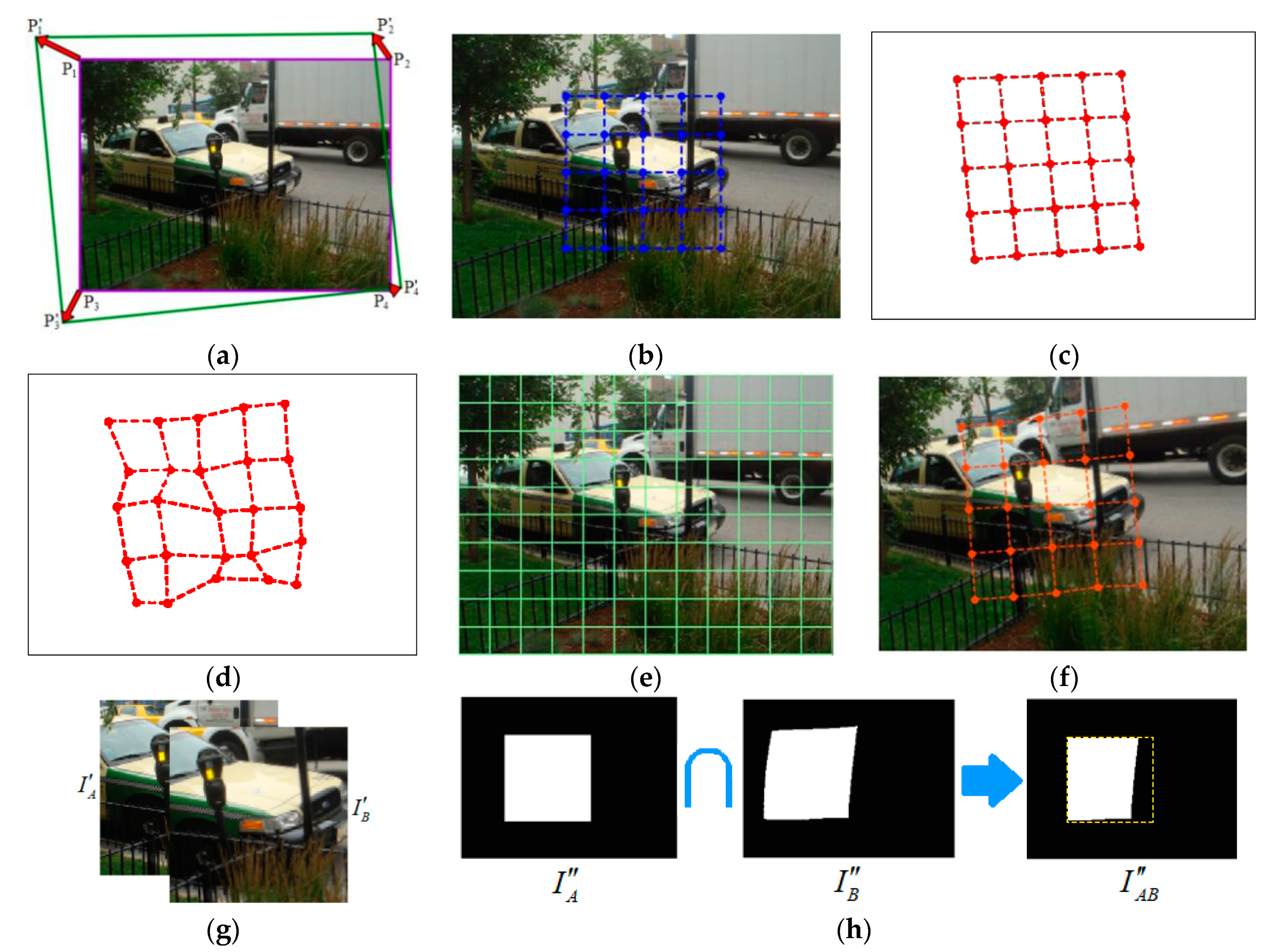
Figure 1. The process of the proposed sample and label generation method: (a) Generate four pairs of points and obtain the corresponding homography matrix H 4 p t A B ; (b) randomly cut out the original image to generate an M × N uniform grid GA; (c) M × N points G A transformed from GA by using H 4 p t A B ; (d) M × N perturbation points G ˜ A generated from G A ; (e) adaptively generate m × n uniform grid; (f) image IB transformed from IA using local homography matrices H L A B ; (g) generated alternative samples; (h) calculation of overlap degree of two sample images.
Applsci 10 00732 g001
Figure 2. Robustness of seven image registration algorithms under different image augmentation degrees: (a) Failure rate; (b) RMSE.
Applsci 10 00732 g002
Figure 3. Robustness of DeTone’s algorithm, Nguyen’s algorithm and the proposed algorithm using VGG: (a) Failure rate; (b) RMSE.
Applsci 10 00732 g003
Figure 4. Robustness of DeTone’s algorithm, Nguyen’s algorithm and the proposed algorithm using Googlenet: (a) Failure rate; (b) RMSE.
Applsci 10 00732 g004
Figure 5. Robustness of DeTone’s algorithm, Nguyen’s algorithm and the proposed algorithm using Xception: (a) Failure rate; (b) RMSE.
Applsci 10 00732 g005
Figure 6. Robustness of the proposed algorithm under different perturbation values and CNNs: (a) ρ = 36; (b) ρ = 32; (c) ρ = 28; (d) ρ = 24.
Applsci 10 00732 g006
Figure 7. Visualization analysis of the proposed algorithm under different CNNs (The red boxes indicate the ground truth, and the yellow boxes are the estimation results): (a) accuracy of image registration under VGG (RMSE = 10.154711); (b) accuracy of image registration under VGG (RMSE = 2.240815); (c) accuracy of image registration under Googlenet (RMSE = 7.2284245); (d) accuracy of image registration under Googlenet (RMSE = 1.9681364); (e) accuracy of image registration under Xception (RMSE = 3.1798978); (f) accuracy of image registration under Xception (RMSE = 1.4085304).
Applsci 10 00732 g007
Table 1. RMSE comparison of different image registration algorithms.
Algorithmic TypeAlgorithmRMSE
Pixel basedECC18.13
Feature basedSIFT5.077
ORB 17.751
APAP4.458
Learning basedDeTone + VGG11.844
DeTone + Googlenet10.512
DeTone + Xception10.011
Nguyen + VGG10.455
Nguyen + Googlenet9.936
Nguyen + Xception9.861
Proposed + VGG6.113
Proposed + Googlenet4.344
Proposed + Xception2.339
Table 2. Running time comparison of different image registration algorithms.
Algorithmic TypeAlgorithmRunning Time of GPU (s)Running Time of CPU (s)
Pixel basedECC-226
Feature basedSIFT-99
ORB -65
APAP-456
Learning basedDeTone + VGG36.2123
DeTone + Googlenet26.957.3
DeTone + Xception46.2208
Nguyen + VGG36.2123
Nguyen + Googlenet26.957.3
Nguyen + Xception46.2208
Proposed + VGG47.2138
Proposed + Googlenet39.761
Proposed + Xception59.6213