Shape Dependence of Falling Snow Crystals’ Microphysical Properties Using an Updated Shape Classification


Abstract
1. Introduction
2. Site and Measurements
2.1. Measurement Site
2.2. Instrument
2.3. Image Processing
3. Particle Shape Classification
3.1. Classification Method
3.2. Recent Updates
3.3. New Shapes from Kiruna
4. Shape Groups
5. Properties of Shape Groups
5.1. Occurrence and Properties
5.2. Relationships between Microphysical Properties
5.2.1. Cross-Sectional Area and Area Ratio
5.2.2. Area Ratio and Aspect Ratio
6. Summary and Conclusions
- The dual images provides more information about the particle shape.
- We found 34 snow particles that are not yet described and that warrant their own shape in the updated shape classification.
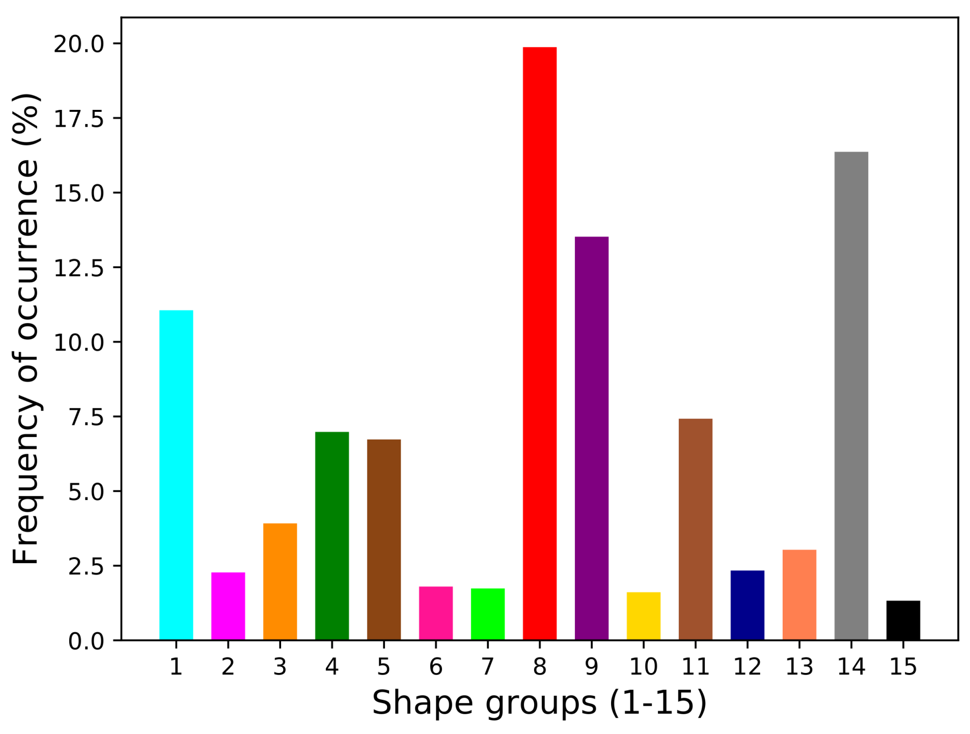
- In our dataset, shape groups (1) Needles and thin or long columns, (8) Branches, (9) Side planes, and (14) Irregulars and aggregates are the most common, occurring more often than 10% of the time.
- Shape group (6) Stellar crystals has the largest median particle size, = 1450 m, followed by shape groups (2) Crossed needles and crossed columns, (7) Bullet rosettes, (8) Branches, (9) Side planes, and (11) Spatial stellar crystals with > 1000 m. Shape groups (3) Thick columns and bullets, (5) Plates, (13) Ice and melting or sublimating particles, and (15) Spherical particles have the smallest < 500 m (see Figure 4a).
- Shape group (6) Stellar crystals also has the largest median cross-sectional area, A = 6.34 , followed by shape groups (7) Bullet rosettes, (8) Branches, (9) Side planes, and (11) Spatial stellar crystals with A > 3.0 (see Figure 4b).
- In general, groups with large particle sizes also have large areas. However, there are exceptional shape groups with the largest particle sizes but with smaller areas, as it is in the case of shape group (2) Crossed needles and crossed columns. We can see in Figure 4c, in which we note that shape groups (1) Needles and thin or long columns, (2) Crossed needles and crossed columns, and (3) Thick columns and bullets have the smallest area ratios, .
- In general, there is a good correlation of the A vs. relationship for the shape groups, with correlation coefficients varying from 0.73 for shape group (2) Crossed needles and crossed columns to over 0.9 for shape groups (5) Plates, (11) Spatial stellar crystals, (12) Graupel, (13) Ice and melting or sublimating particles, (14) Irregulars and aggregates, and (15) Spherical particles (see Table 9).
- In most shape groups, area ratio decreases with increasing particle size. This is strongest for the shape groups with the lowest area ratios: (1) Needles and thin or long columns, (2) Crossed needles and crossed columns, and (3) Thick columns and bullets, which consequently also have the lowest values of . The shape groups (15) Spherical particles, (14) Graupel, and (6) Stellar crystals are exceptions and have area ratios that are almost constant.
- Shape groups (1) Needles and thin or long columns, (3) Thick columns and bullets, (5) Plates, and (15) Spherical particles have the highest correlation in the vs. relationship, with larger than 0.8 (see Table 9). On the other hand, shape groups (2) Crossed needles and crossed columns, (6) Stellar crystals, (7) Bullet rosettes, and (9) Side planes have correlation coefficients lower than 0.5. Shape groups (6) Stellar crystals and (7) Bullet rosettes have a particularly low vs. correlation of 0.25 despite a A vs. correlation larger than 0.82. For instance, in the case of the shape group (6) Stellar crystals, this might be due to several factors; the empty space between their branches resulting in low values and/or variations in due to particle orientation.
Author Contributions
Funding
Acknowledgments
Conflicts of Interest
Appendix A. Shapes


| Level (N, C, …), Sublevel (1, 2, …), Name | Label |
|---|---|
| N = Needle crystal | |
| 1. Simple needle | |
| a. Elementary needle | N1a |
| b. Bundle of elementary needles | N1b |
| c. Elementary sheath | N1c |
| d. Bundle of elementary sheaths | N1d |
| e. Long solid column | N1e |
| 2. Combination of needle crystals | |
| a. Combination of needles | N2a |
| b. Combination of sheaths | N2b |
| c. Combination of long solid columns | N2c |
| C = Columnar crystal | |
| 1. Simple column | |
| a. Pyramid | C1a |
| b. Cup | C1b |
| c. Solid bullet | C1c |
| d. Hollow bullet | C1d |
| e. Solid column | C1e |
| f. Hollow column | C1f |
| g. Solid thick plate | C1g |
| h. Thick plate of skeleton form | C1h |
| i. Scroll | C1i |
| j. Twin columns | C1j [Li] |
| 2. Combination of columns | |
| a. Combination of bullets (bullet rosettes) | C2a |
| b. Combination of columns (column rosettes) | C2b |
| P = Plane crystal | |
| 1. Regular crystal developed in one plane | |
| a. Hexagonal plate | P1a |
| b. Crystal with sector-like branches | P1b |
| c. Crystal with broad branches | P1c |
| d. Stellar crystal | P1d |
| e. Ordinary dendritic crystal | P1e |
| f. Fernlike crystal | P1f |
| g. Triangular form/plate | P1g [Li] |
| h. Rectangular plate | P1h [KRN] |
| i. Hollow plate | P1i [Li] |
| j. Plate with a central hole | P1j [KRN] |
| k. Split plate | P1k [Li] |
| l. Split stellar crystal | P1l [Li] |
| m. Irregular split plate | P1m [KRN] |
| n. Irregular split stellar crystal | P1n [KRN] |
| o. Double plate | P1o [Li] |
| p. Double stellar crystal | P1p [KRN] |
| q. Stellar over plate | P1q [KRN] |
| 2. Plane crystal with extensions of different form | |
| a. Stellar crystal with plates at ends | P2a |
| b. Stellar crystal with sector-like ends | P2b |
| c. Dendritic crystal with plates at ends | P2c |
| d. Dendritic crystal with sector-like ends | P2d |
| e. Plate with simple extensions | P2e |
| f. Plate with sector-like extensions | P2f |
| g. Plate with dendritic extensions | P2g |
| h. Triangular form with plates at ends | P2h [KRN] |
| i. Triangular form with dendrites at ends | P2i [KRN] |
| j. Concentric plates with sector-like extensions | P2j [KRN] |
| k. Concentric plates with stellar or dendritic extensions | P2k [KRN] |
| 3. Crystals with irregular number of branches | |
| a. Two-branched crystal | P3a |
| b. Three-branched crystal | P3b |
| c. Four-branched crystal | P3c |
| 4. Crystal with 12 branches | |
| a. Broad branch crystal with 12 branches | P4a |
| b. Dendritic crystal with 12 branches | P4b |
| 5. Malformed crystal | |
| Many varieties | P5 |
| 6. Spatial assemblage of plane branches | |
| a. Plate with spatial plates | P6a |
| b. Plate with spatial dendrites | P6b |
| c. Stellar crystal with spatial plates | P6c |
| d. Stellar crystal with spatial dendrites | P6d |
| 7. Radiating assemblage of plane branches | |
| a. Radiating assemblage of plates | P7a |
| b. Radiating assemblage of dendrites | P7b |
| CP = Combination of column and plane crystals | |
| 1. Column with plane crystals at both ends | |
| a. Column with plates (capped column) | CP1a |
| b. Column with dendrites | CP1b |
| c. Multiple capped column | CP1c |
| d. Column with plate and dendrite | CP1d [KRN] |
| e. Asymmetric capped column (with plates) | CP1e [KRN] |
| f. Multiple capped column with dendrites | CP1f [KRN] |
| g. Asymmetric column with dendrites | CP1g [KRN] |
| 2. Bullet with plane crystals | |
| a. Bullet with plate | CP2a [Ki] |
| b. Bullet with dendrite | CP2b |
| c. Bullet with plate and dendrite | CP2c [KRN] |
| d. Bullet with two plates | CP2d [KRN] |
| e. Bullet with two dendrites | CP2e [KRN] |
| f. Combination of bullets (capped bullets) | CP2f [KRN] |
| g. Combination of bullets with plates | CP2g [Ki] |
| h. Combination of bullets with dendrites | CP2h [Ki] |
| i. Asymmetric combination of bullets | CP2i [KRN] |
| 3. Plane crystal with spatial extensions at ends | |
| a. Stellar crystal (dendrite) with needles | CP3a |
| b. Stellar crystal (dendrite) with columns | CP3b |
| c. Stellar crystal (dendrite) with scrolls at ends | CP3c |
| d. Plate with needles | CP3d [Ki] |
| e. Plate with columns | CP3e [Ki] |
| f. Plate with scrolls at ends | CP3f |
| 4. Seagull-type crystal | |
| a. Seagull crystal | CP4a [Ki] |
| S = Columnar crystals with extended side planes | |
| 1. Side planes | S1 |
| 2. Scale-like side planes | S2 |
| 3. Combination of side planes, bullets, and columns | S3 |
| 4. Arrowhead twins | S4 [Li] |
| 5. Crossed plates | S5 [Li] |
| A = Aggregates of snow crystals | |
| 1. Aggregation of column-type crystals | |
| a. Aggregation of combinations of columns and bullets | A1a [Ki] |
| 2. Aggregation of plane-type crystals | |
| a. Aggregation of combinations of plates and dendrites | A2a [Ki] |
| 3. Aggregation of column- and plane-type crystals | |
| a. Aggregation of combinations of columns, | A3a [Ki] |
| planes and crossed plates | |
| 4. Aggregation of multiple capped columns | |
| a. Aggregation of multiple capped columns | A4a [KRN] |
| 5. Aggregation of needle- and sheath-type crystals | |
| a. Aggregation of needles and sheaths | A5a [KRN] |
| 6. Aggregation of stellar-type crystals | |
| a. Aggregation of stellar crystals | A6a [KRN] |
| 7. Aggregation of dendrite-type crystals | |
| a. Aggregation of dendrite crystals | A7a [KRN] |
| 8. Aggregation of plate-type crystals | |
| a. Aggregation of plates | A8a [KRN] |
| 9. Aggregation of bullet-type crystals | |
| a. Aggregation of bullets | A9a [KRN] |
| b. Aggregation of bullet rosettes and capped bullets | A9b [KRN] |
| 10. Aggregation of branch-type crystals | |
| a. Aggregation of branches | A10a [KRN] |
| 11. Aggregation of seagull-type crystals | |
| a. Aggregation of seagull | A11a [KRN] |
| 12. Aggregation of malformed-type crystals | |
| a. Aggregation of malformed crystals | A12a [KRN] |
| 13. Aggregation of irregular-type crystals | |
| a. Aggregation of irregular particles | A13a [KRN] |
| 14. Aggregation of frozen small raindrops | |
| and snow crystals | |
| a. Aggregation of frozen small raindrops | A14a [KRN] |
| and snow crystals | |
| R = Rimed crystal (crystal with cloud droplets attached) | |
| 1. Rimed crystal | |
| a. Rimed needle crystal | R1a |
| b. Rimed columnar crystal | R1b |
| c. Rimed plate or sector | R1c |
| d. Rimed stellar crystal | R1d |
| e. Rimed bundle | R1e [KRN] |
| f. Rimed capped bullet | R1f [KRN] |
| 2. Densely rimed crystal | |
| a. Densely rimed plate or sector | R2a |
| b. Densely rimed stellar crystal | R2b |
| c. Stellar crystal with rimed spatial branches | R2c |
| 3. Graupel-like snow | |
| a. Graupel-like snow of hexagonal type | R3a |
| b. Graupel-like snow of lump type | R3b |
| c. Graupel-like snow with non-rimed extensions | R3c |
| 4. Graupel | |
| a. Hexagonal graupel | R4a |
| b. Lump graupel | R4b |
| c. Cone-like graupel | R4c |
| I = Irregular snow crystal | |
| 1. Ice particle | I1 |
| 2. Rimed particle | I2 |
| 3. Broken piece from a crystal | |
| a. Broken branch | I3a |
| b. Rimed broken branch | I3b |
| 4. Miscellaneous | I4 |
| G = Germ of snow crystal (ice crystal) | |
| 1. Minute column | G1 |
| 2. Germ of skeleton form | G2 |
| 3. Minute hexagonal plate | G3 |
| 4. Minute stellar crystal | G4 |
| 5. Minute assemblage of plates | G5 |
| 6. Irregular germ | G6 |
| H = Other solid precipitation particles | |
| 1. Frozen hydrometeor particle | |
| a. Frozen cloud particle | H1a [Ki] |
| b. Chained frozen cloud particles | H1b [Ki] |
| c. Frozen small raindrop | H1c [Ki] |
| 2. Sleet particle | |
| a. Sleet particle | H2a [Ki] |
| 3. Ice pellet | |
| a. Ice pellet | H3a [Ki] |
| 4. Droplets of water | |
| a. Raindrop | H4a [KRN] |
Appendix B. Shape Groups
| Shape Groups (1–15), Name | Label |
|---|---|
| (1) Needles and thin or long column | |
| Elementary needle | N1a |
| Bundle of elementary needles | N1b |
| Elementary sheath | N1c |
| Bundle of elementary sheaths | N1d |
| Long solid column | N1e |
| Rimed needle crystal | R1a |
| Rimed columnar crystal | R1b |
| Rimed bundle | R1e [KRN] |
| (2) Crossed needles and crossed columns | |
| Combination of needles | N2a |
| Combination of sheaths | N2b |
| Combination of long solid columns | N2c |
| (3) Thick columns and bullets | |
| Pyramid | C1a |
| Cup | C1b |
| Solid bullet | C1c |
| Hollow bullet | C1d |
| Solid column | C1e |
| Hollow column | C1f |
| Solid thick plate | C1g |
| Scroll | C1i |
| Twin columns | C1j [Li] |
| Minute column | G1 |
| (4) Capped columns and capped bullets | |
| Column with plates (capped column) | CP1a |
| Column with dendrites | CP1b |
| Multiple capped column | CP1c |
| Column with plate and dendrite | CP1d [KRN] |
| Asymmetric capped column (with plates) | P1e [KRN] |
| Multiple capped column with dendrites | CP1f [KRN] |
| Asymmetric column with dendrites | CP1g [KRN] |
| Bullet with plate | CP2a [Ki] |
| Bullet with dendrite | CP2b |
| Bullet with plate and dendrite | CP2c [KRN] |
| Bullet with two plates | CP2d [KRN] |
| Bullet with two dendrites | CP2e [KRN] |
| Combination of bullets (capped bullets) | CP2f [KRN] |
| (5) Plates | |
| Thick plate of skeleton form | C1h |
| Hexagonal plate | P1a |
| Crystal with sector-like branches | P1b |
| Crystal with broad branches | P1c |
| Triangular form/plate | P1g [Li] |
| Rectangular plate | P1h [KRN] |
| Hollow plate | P1i [Li] |
| Plate with a central hole | P1j [KRN] |
| Split plate | P1k [Li] |
| Irregular split plate | P1m [KRN] |
| Double plate | P1o [Li] |
| Stellar crystal over plate | P1q [KRN] |
| Plate with scrolls at ends | CP3f |
| Rimed plate or sector | R1c |
| Germ of skeleton from | G2 |
| Minute hexagonal plate | G3 |
| (6) Stellar crystals | |
| Stellar crystal | P1d |
| Ordinary dendritic crystal | P1e |
| Fernlike crystal | P1f |
| Split stellar crystal | P1l [Li] |
| Irregular split stellar crystal | P1n [KRN] |
| Double stellar crystal | P1p [KRN] |
| Stellar crystal with plates at ends | P2a |
| Stellar crystal with sector-like ends | P2b |
| Dendritic crystal with plates at ends | P2c |
| Dendritic crystal with sector-like ends | P2d |
| Plate with simple extensions | P2e |
| Plate with sector-like extensions | P2f |
| Plate with dendritic extensions | P2g |
| Triangular form with plates at ends | P2h [KRN] |
| Triangular form with dendrites at ends | P2i [KRN] |
| Concentric plates with sector-like extensions | P2j [KRN] |
| Concentric plates with stellar or dendritic extensions | P2k [KRN] |
| Broad branch crystal with 12 branches | P4a |
| Dendritic crystal with 12 branches | P4b |
| Stellar crystal with scrolls at ends | CP3c |
| Rimed stellar crystal | R1d |
| Minute stellar crystal | G4 |
| (7) Bullet rosettes | |
| Combination of bullets (bullet rosettes) | C2a |
| Combination of columns (column rosettes) | C2b |
| Combination of bullets with plates | CP2g [Ki] |
| Combination of bullets with dendrites | CP2h [Ki] |
| Asymmetric combination of bullets | CP2i [KRN] |
| Rimed capped bullet | R1f [KRN] |
| (8) Branches | |
| Two-branched crystal | P3a |
| Three-branched crystal | P3b |
| Four-branched crystal | P3c |
| Malformed crystal | P5 |
| Radiating assemblage of dendrites | P7b |
| Seagull crystal | CP4a [Ki] |
| Broken branch | I3a |
| Rimed broken branch | I3b |
| (9) Side planes | |
| Radiating assemblage plates | P7a |
| Side planes | S1 |
| Scale-like side planes | S2 |
| Combination of side planes, bullets, and columns | S3 |
| Arrowhead twins | S4 [Li] |
| Crossed plates | S5 [Li] |
| Minute assemblage of plates | G5 |
| (10) Spatial plates | |
| Plate with spatial plates | P6a |
| Plate with spatial dendrites | P6b |
| Plate with needles | CP3d [Ki] |
| Plate with columns | CP3e [Ki] |
| Densely rimed plate or sector | R2a |
| (11) Spatial stellar crystals | |
| Stellar crystal with spatial plates | P6c |
| Stellar crystal with spatial dendrites | P6d |
| Stellar crystal with needles | CP3a |
| Stellar crystal with columns | CP3b |
| Densely rimed stellar crystal | R2b |
| Stellar crystal with rimed spatial branches | R2c |
| Graupel-like snow of hexagonal type | R3a |
| Graupel-like snow of lump type | R3b |
| Graupel-like snow with non-rimed extensions | R3c |
| (12) Graupel | |
| Hexagonal graupel | R4a |
| Lump graupel | R4b |
| Cone-like graupel | R4c |
| (13) Ice and melting or sublimating particles | |
| Ice particle | I1 |
| Frozen cloud particle | H1a [Ki] |
| Chained frozen cloud particles | H1b [Ki] |
| Sleet particle | H2a [Ki] |
| Ice pellet | H3a [Ki] |
| (14) Irregulars and aggregates | |
| Aggregation of combinations of columns and bullets | A1a [Ki] |
| Aggregation of combinations of plates and dendrites | A2a [Ki] |
| Aggregation of combinations of columns, planes and crossed plates | A3a [Ki] |
| Aggregation of multiple capped columns | A4a [KRN] |
| Aggregation of needles and sheaths | A5a [KRN] |
| Aggregation of stellar crystals | A6a [KRN] |
| Aggregation of dendrite crystals | A7a [KRN] |
| Aggregation of plates | A8a [KRN] |
| Aggregation of bullets | A9a [KRN] |
| Aggregation of bullet rosettes and capped bullets | A9b [KRN] |
| Aggregation of branches | A10a [KRN] |
| Aggregation of seagull | A11a [KRN] |
| Aggregation of malformed crystals | A12a [KRN] |
| Aggregation of irregular particles | A13a [KRN] |
| Aggregation of frozen small raindrops and snow crystals | A14a [KRN] |
| Rimed particle | I2 |
| Miscellaneous | I4 |
| Irregular germ | G6 |
| (15) Spherical particles | |
| Frozen small raindrop | H1c [Ki] |
| Raindrop | H4a [KRN] |
References
- Stoelinga, M.; Hobbs, P.V.; Mass, C.F.; Locatelli, J.; Colle, B.; Houze, R.; Rangno, A.L.; Bond, N.A.; Smull, B.F.; Rasmussen, R.M.; et al. Improvement of Microphysical Parameterization through Observational Verification Experiment (IMPROVE). Bull. Am. Met. Soc. 2003, 84, 1807–1826. [Google Scholar] [CrossRef]
- Tao, W.K.; Simpson, J.; Baker, D.; Braun, S.; Chou, M.D.; Ferrier, B.; Johnson, D.; Khain, A.; Lang, S.; Lynn, B.; et al. Microphysics, radiation and surface processes in the Goddard Cumulus Ensemble (GCE) model. Meteorol. Atmos. Phys. 2003, 82, 97–137. [Google Scholar] [CrossRef]
- Posselt, D.J.; L’Ecuyer, T.S.; Stephens, G.L. Exploring the error characteristics of thin ice cloud property retrievals using a Markov chain Monte Carlo algorithm. J. Geophys. Res. 2008, 113. [Google Scholar] [CrossRef]
- Zhang, Z.; Yang, P.; Kattawar, G.; Riedi, J.; Labonnote, L.C.; Baum, B.A.; Platnick, S.; Huang, H.L. Influence of ice particle model on satellite ice cloud retrieval: lessons learned from MODIS and POLDER cloud product comparison. Atmos. Chem. Phys. 2009, 9, 7115–7129. [Google Scholar] [CrossRef]
- Cooper, S.J.; Garrett, T.J. Identification of small ice cloud particles using passive radiometric observations. J. Appl. Meteorol. 2010, 49, 2334–2347. [Google Scholar] [CrossRef]
- IPCC. Clouds and Aerosols. In Climate Change 2013—The Physical Science Basis: Working Group I Contribution to the Fifth Assessment Report of the Intergovernmental Panel on Climate Change; Cambridge University Press: Cambridge, UK, 2014; pp. 571–658. [Google Scholar] [CrossRef]
- Pruppacher, H.R.; Klett, J.D. Microphysics of Clouds and Precipitation, 2nd ed.; Kluwer Academic Publishers: Dordrecht, The Netherlands, 1997. [Google Scholar]
- Nakaya, U.; Sekido, Y. General Classification of Snow Crystals and their Frequency of Occurrence. J. Fac. Sci. Hokkaido Imp. Univ. Ser. II 1936, 1, 243–264. [Google Scholar]
- Hanajima, M. On the conditions for the formation of snow crystals. J. Meteorol. Soc. Jpn. Ser. II 1942, 20, 238–251. [Google Scholar] [CrossRef]
- Nakaya, U. Snow Crystal Growth: Electron Microscope Study of Snow Crystal Nuclei (Advance communication). J. Glaciol. 1951, 1, 550. [Google Scholar] [CrossRef][Green Version]
- Nakaya, U. The Formation of Ice Crystals; American Meteorological Society: Boston, MA, USA, 1951; pp. 207–220. [Google Scholar] [CrossRef]
- Itoo, K. On the Growth of Ice Crystals in the Air. Pap. Meteor. Geophys. 1951, 2, 315–316. [Google Scholar] [CrossRef][Green Version]
- Isono, K. An Electron–Microscope Study of Ice Crystal Formation – A Preliminary Report. J. Meteorol. Soc. Jpn. Ser. II 1953, 31, 318–322. [Google Scholar] [CrossRef]
- Isono, K. On the Growth of Ice-Crystals in the Air. J. Meteorol. Soc. Jpn. Ser. II 1957, 35A, 31–37. [Google Scholar] [CrossRef]
- Ukitiro, N.; Masando, H.; Jiro, M. Physical Investigations on the Growth of Snow Crystals. J. Fac. Sci. Hokkaido Univ. Ser. II 1958, 5, 88–118. [Google Scholar]
- Libbrecht, K.G. Morphogenesis on Ice: The Physics of Snow Crystals. Eng. Sci. 2001, I, 10–19. [Google Scholar]
- Libbrecht, K.G. The physics of snow crystals. Rep. Prog. Phys. 2005, 68, 855–895. [Google Scholar] [CrossRef]
- Seasonal Snow Cover: a guide for measurement compilation and assemblage of data. Unesco/IASH/WMO, 1970. Available online: https://globalcryospherewatch.org/bestpractices/docs/UNESCO_snow_cover_1970.pdf (accessed on 4 December 2019).
- Fierz, C.; Armstrong, R.; Durand, Y.; Etchevers, P.; Greene, E.; McClung, D.; Nishimura, K.; Satyawali, P.; Sokratov, S. The International Classification for Seasonal Snow on the Ground (UNESCO, IHP (International Hydrological Programme)—VII, Technical Documents in Hydrology, No 83); IACS (International Association of Cryospheric Sciences) Contribution No 1; UNESCO/Division of Water Sciences: Paris, France, 2009. [Google Scholar]
- Magono, C.; Lee, C.W. Meteorological classification of natural snow crystals. J. Fac. Sci. Hokkaido Univ. 1966, II, 321–335. [Google Scholar]
- Kikuchi, K.; Kameda, T.; Higuchi, K.; Yamashita, A. A global classification of snow crystals, ice crystals, and solid precipitation based on observations from middle latitudes to polar regions. Atmos. Res. 2013, 132–133, 460–472. [Google Scholar] [CrossRef]
- Kuhn, T.; Vázquez-Martín, S. Microphysical properties and fall speed measurements of snow ice crystals using the Dual Ice Crystal Imager (D-ICI). Atmos. Meas. Tech. Discuss. 2019, 1–24. [Google Scholar] [CrossRef]
- Libbrecht, K.G. Ken Libbrecht’s Field Guide to Snowflakes; Voyageur Press: Minneapolis, MN, USA, 2006. [Google Scholar]
- SMHI. Januari 2018—Lufttemperatur och vind, SMHI_vov_temperature_wind_jan18. Available online: https://www.ce.se/smhi-sveriges-meteorologiska-och-hydrologiska-institut/ (accessed on 4 December 2019).
- IRF. Weather at IRF. Available online: http://www2.irf.se/weather/ (accessed on 4 December 2019).
- Kuhn, T.; Gultepe, I. Ice Fog and Light Snow Measurements Using a High-Resolution Camera System. Pure Appl. Geophys. 2016, 173, 3049–3064. [Google Scholar] [CrossRef]


| Particle Shape Name (Old Label) | New Label |
|---|---|
| Kikuchi et al. [21]: | |
| Combination of bullets with plates (CP2c) | CP2f |
| Combination of bullet with dendrites (CP2d) | CP2g |
| Seagull-type crystals (CP9a–CP9e) | CP4a |
| Bullet with plate | CP2a |
| Plate with needles | CP3d |
| Plate with columns | CP3e |
| Aggregation of combinations of columns and bullets | A1a |
| Aggregation of combinations of plates and dendrites | A2a |
| Aggregation of combinations of columns, planes and | A3a |
| crossed plates | |
| Frozen cloud particle | H1a |
| Chained frozen cloud particles | H1b |
| Frozen small raindrop | H1c |
| Sleet particle | H2a |
| Ice pellet | H3a |
| Libbrecht [23]: | |
| Twin columns | C1j |
| Triangular form/plate | P1g |
| Hollow plate | P1i |
| Split plate | P1k |
| Split stellar crystal | P1l |
| Double plate | P1o |
| Arrowhead twins | S4 |
| Crossed plates | S5 |
| Particle Shape Name | New Label |
|---|---|
| Rectangular plate | P1h |
| Plate with a central hole | P1j |
| Irregular split plate | P1m |
| Irregular split stellar crystal | P1n |
| Double stellar crystal | P1p |
| Stellar over plate | P1q |
| Triangular form with plates at ends | P2h |
| Triangular form with dendrites at ends | P2i |
| Concentric plates with sector-like extensions | P2j |
| Concentric plates with stellar or dendritic extensions | P2k |
| Column with plate and dendrite | CP1d |
| Asymmetric capped column (with plates) | CP1e |
| Multiple capped column with dendrites | CP1f |
| Asymmetric column with dendrites | CP1g |
| Bullet with plate and dendrite | CP2c |
| Bullet with two plates | CP2d |
| Bullet with two dendrites | CP2e |
| Combination of bullets (capped bullets) | CP2f |
| Asymmetric combination of bullets | CP2i |
| Aggregation of multiple capped columns | A4a |
| Aggregation of needles and sheaths | A5a |
| Aggregation of stellar crystals | A6a |
| Aggregation of dendrite crystals | A7a |
| Aggregation of plates | A8a |
| Aggregation of bullets | A9a |
| Aggregation of bullet rosettes and capped bullets | A9b |
| Aggregation of branches | A10a |
| Aggregation of seagull | A11a |
| Aggregation of malformed crystals | A12a |
| Aggregation of irregular particles | A13a |
| Aggregation of frozen small raindrops and snow crystals | A14a |
| Rimed bundle | R1e |
| Rimed capped bullet | R1f |
| Raindrop | H4a |
| Shape Groups (1–15) |
|---|
| (1) Needles and thin or long columns |
| (2) Crossed needles and crossed columns |
| (3) Thick columns and bullets |
| (4) Capped columns and capped bullets |
| (5) Plates |
| (6) Stellar crystals |
| (7) Bullet rosettes |
| (8) Branches |
| (9) Side planes |
| (10) Spatial plates |
| (11) Spatial stellar crystals |
| (12) Graupel |
| (13) Ice and melting or sublimating particles |
| (14) Irregulars and aggregates |
| (15) Spherical particles |
| Shape Groups (1–15) and their Descriptions | Images |
|---|---|
| (1) Needles and thin or long columns: Includes needles, other snow crystals with elongated features (i.e., needle-like shape), and thin or long columns, including rimed needles and rimed thin columnar crystals. |  |
| (2) Crossed needles and crossed columns: Combination of crossed needles and a combination of crossed thin or long columns. |  |
| (3) Thick columns and bullets: Thick columnar, minute columns, bullet shape, scroll, pyramid, and cup shapes. |  |
| (4) Capped columns and capped bullets: Columns and bullets with plates at one end or both ends. |  |
| (5) Plates: Hexagonal plates including solid and hollow plates, skeletal surfaces, sector plates, plates with scrolls at the end, rimed plates, split plates, double plates, concentric plates, minute hexagonal plate, plate ice crystal, and triangular and rectangular plates. |  |
| Shape Groups (1–15) and their Descriptions | Images |
|---|---|
| (6) Stellar crystals: Stellar and dendrite shapes including simple stars, stellar with plates or sector-like ends, dendritic crystal with plates or sector-like ends, plate with simple, sector-like or dendritic extensions, broad branch or dendritic crystal with 12 branches, stellar crystal with scrolls at ends, rimed stellar crystal, split stellar crystals, double stellar crystal, concentric plates with extensions of different forms, minute stellar crystal, dendrite ice crystal, and triangular form with extensions of different forms. |  |
| (7) Bullet rosettes: Combination of bullets or columns, bullet rosette shapes including bullet with plates or dendrites. |  |
| (8) Branches: Arm-extension-like shape, malformed dendritic crystal, and seagull-type crystal. |  |
| Shape Groups (1–15) and their Descriptions | Images |
|---|---|
| (9) Side planes: Snow crystals composed of several crossed hexagonal plates including radiating plates, side planes, scale-like side planes, combination of side planes with bullets and columns, assemblage of plates, arrowhead twins, and crossed plates shape. |  |
| (10) Spatial plates: Snow crystals composed of a plate with spatially attached plates or dendrites including densely rimed plate and columns on plates. |  |
| (11) Spatial stellar crystals: Stellar crystal or dendrites with spatial plates or with dendrites, including densely rimed stellar crystal, stellar crystal with rimed spatial branches, graupel-like snow of hexagonal type or lump type, and graupel-like snow with non-rimed extensions. |  |
| (12) Graupel: Soft hail shape considering that perceptions and definitions of soft hail can vary. |  |
| Shape Groups (1–15) and their Descriptions | Images |
|---|---|
| (13) Ice and melting or sublimating particles: Minute ice crystals, i.e., particles that grow in cirrus clouds from minute frozen cloud droplets, such as frozen cloud particles, and ice pellets. |  |
| (14) Irregulars and aggregates: Particles that cannot be classified into any other shape group in addition of the agglomeration of snow crystals. |  |
| (15) Spherical particles: Frozen small raindrops and liquid raindrops. |  |
| Shape Groups (1–15) | # | /m | A/ m | |||||||
|---|---|---|---|---|---|---|---|---|---|---|
| Median | 15.9% | 84.1% | Median | 15.9% | 84.1% | Median | 15.9% | 84.1% | ||
| (1) Needles/long columns | 350 | 956 | 555 | 1485 | 142 | 81.3 | 232 | 0.195 | 0.119 | 0.363 |
| (2) Crossed needles/col. | 72 | 1267 | 910 | 1737 | 233 | 148 | 357 | 0.181 | 0.124 | 0.282 |
| (3) Thick columns | 124 | 473 | 283 | 659 | 69.0 | 34.1 | 105 | 0.411 | 0.281 | 0.654 |
| (4) Capped columns/bull. | 221 | 662 | 476 | 1084 | 175 | 89.1 | 393 | 0.498 | 0.332 | 0.666 |
| (5) Plates | 213 | 504 | 336 | 856 | 143 | 65.7 | 387 | 0.748 | 0.596 | 0.823 |
| (6) Stellar crystals | 57 | 1450 | 864 | 1876 | 634 | 235 | 1260 | 0.443 | 0.315 | 0.561 |
| (7) Bullet rosettes | 55 | 1040 | 724 | 1305 | 348 | 194 | 570 | 0.430 | 0.326 | 0.561 |
| (8) Branches | 629 | 1078 | 714 | 1589 | 360 | 170 | 748 | 0.415 | 0.313 | 0.526 |
| (9) Side planes | 428 | 1105 | 856 | 1470 | 432 | 255 | 773 | 0.462 | 0.368 | 0.573 |
| (10) Spatial plates | 51 | 699 | 500 | 978 | 239 | 131 | 422 | 0.659 | 0.544 | 0.758 |
| (11) Spatial stellar cryst. | 235 | 1032 | 621 | 1683 | 420 | 168 | 1040 | 0.521 | 0.431 | 0.599 |
| (12) Graupel | 74 | 571 | 390 | 912 | 156 | 75.6 | 435 | 0.646 | 0.597 | 0.719 |
| (13) Ice/melting particles | 96 | 279 | 212 | 509 | 40.2 | 21.2 | 95.5 | 0.596 | 0.384 | 0.765 |
| (14) Irregulars/aggregates | 518 | 821 | 503 | 1452 | 247 | 97.6 | 619 | 0.488 | 0.337 | 0.618 |
| (15) Spherical particles | 42 | 181 | 108 | 236 | 24.8 | 8.60 | 48.7 | 0.961 | 0.924 | 0.976 |
| All shape groups together | ||||||||||
| (regardless of shape) | 3165 | 899 | 489 | 1454 | 244 | 89.7 | 614 | 0.461 | 0.286 | 0.640 |
| Shape Groups (1–15) | A vs. | vs. | ||||
|---|---|---|---|---|---|---|
| / | ||||||
| (1) Needles and thin or long columns | 108 | 1.05 | 0.76 | 0.0183 | 0.698 | 0.90 |
| (2) Crossed needles and crossed columns | 128 | 1.05 | 0.73 | 0.0591 | 0.252 | 0.32 |
| (3) Thick columns and bullets | 31.6 | 1.25 | 0.85 | 0.0415 | 0.756 | 0.89 |
| (4) Capped columns and capped bullets | 5.31 | 1.59 | 0.79 | 0.0120 | 0.654 | 0.46 |
| (5) Plates | 3.17 | 1.72 | 0.94 | −0.00869 | 0.894 | 0.80 |
| (6) Stellar crystals | 0.531 | 1.93 | 0.86 | 0.123 | 0.395 | 0.25 |
| (7) Bullet rosettes | 5.35 | 1.60 | 0.82 | 0.0991 | 0.450 | 0.25 |
| (8) Branches | 2.11 | 1.73 | 0.84 | 0.0845 | 0.483 | 0.47 |
| (9) Side planes | 1.88 | 1.76 | 0.88 | 0.124 | 0.457 | 0.32 |
| (10) Spatial plates | 4.64 | 1.66 | 0.86 | 0.0718 | 0.698 | 0.61 |
| (11) Spatial stellar crystals | 1.88 | 1.78 | 0.95 | 0.0736 | 0.556 | 0.55 |
| (12) Graupel | 0.324 | 1.97 | 0.98 | 0.201 | 0.518 | 0.45 |
| (13) Ice and melting or sublimating particles | 5.87 | 1.54 | 0.91 | 0.0351 | 0.769 | 0.68 |
| (14) Irregulars and aggregates | 3.54 | 1.66 | 0.90 | 0.0158 | 0.648 | 0.52 |
| (15) Spherical particles | 0.795 | 1.99 | 0.99 | −0.168 | 1.14 | 0.93 |
| All shape groups together | ||||||
| (regardless of shape) | 5.66 | 1.58 | 0.83 | −0.451 | 0.900 | 0.71 |
© 2020 by the authors. Licensee MDPI, Basel, Switzerland. This article is an open access article distributed under the terms and conditions of the Creative Commons Attribution (CC BY) license (http://creativecommons.org/licenses/by/4.0/).
Share and Cite
Vázquez-Martín, S.; Kuhn, T.; Eliasson, S. Shape Dependence of Falling Snow Crystals’ Microphysical Properties Using an Updated Shape Classification. Appl. Sci. 2020, 10, 1163. https://doi.org/10.3390/app10031163
Vázquez-Martín S, Kuhn T, Eliasson S. Shape Dependence of Falling Snow Crystals’ Microphysical Properties Using an Updated Shape Classification. Applied Sciences. 2020; 10(3):1163. https://doi.org/10.3390/app10031163
Chicago/Turabian StyleVázquez-Martín, Sandra, Thomas Kuhn, and Salomon Eliasson. 2020. "Shape Dependence of Falling Snow Crystals’ Microphysical Properties Using an Updated Shape Classification" Applied Sciences 10, no. 3: 1163. https://doi.org/10.3390/app10031163
APA StyleVázquez-Martín, S., Kuhn, T., & Eliasson, S. (2020). Shape Dependence of Falling Snow Crystals’ Microphysical Properties Using an Updated Shape Classification. Applied Sciences, 10(3), 1163. https://doi.org/10.3390/app10031163