Article

Wind Pressure Coefficient on a Multi-Storey Building with External Shading Louvers

College of Mechanical and Energy Engineering, Jimei University, Xiamen 361021, China
*
Author to whom correspondence should be addressed.
Appl. Sci. 2020, 10(3), 1128; https://doi.org/10.3390/app10031128
Submission received: 14 January 2020 / Revised: 31 January 2020 / Accepted: 2 February 2020 / Published: 7 February 2020
(This article belongs to the Section Environmental Sciences)

Abstract

:
Wind characteristics on building surfaces are used to evaluate natural ventilation of a building. As a type of building component, external shading louvers are applied in hot climatic regions to block solar radiation and provide better visual environments. The structure of external louvers can affect wind-induced characteristics, such as convective heat transfer coefficient, wind pressure and pollutant dispersion around building envelopes. This paper aims to analyze the potential ventilation capacity of a multi-storey building with shading louvers, based on wind pressure coefficient by the numerical method. A reference case was established and a previous study was applied to validate the numerical results. The rotation angle of horizontal louvers is taken from 0° to 75° in the simulation cases. The results show that average wind pressure has the greatest reduction for all floors when rotation angle turns from 60° to 75°. Ventilation openings on the stagnation zone contribute to higher ventilation rates for the windward facade with louvers. The analysis, based on multi-floor and multi-row buildings under shaded conditions, will provide a greater perspective for engineers to make optimal natural ventilation routes in multi-storey buildings with external shading louvers.

1. Introduction

Building energy use accounts for a great part of energy consumption [1]. Ventilating and shading are two effective methods to reduce building energy use of air-conditioning systems. In hot climatic regions, shading devices are widely used as they can block solar radiation and reduce heat gain, especially for glazed facades, on which the cooling loads account for much higher energy consumption in summer [2]. Several types of shading devices, such as shading louvers, can disperse solar beams and create homogenous daylight distribution in all seasons. Therefore, shading louvers are also applied in other climate regions to provide a better visual environment [3]. The previous research in shading devices mainly focused on the potentialities of energy saving [4], environmental influences [5], optical and thermal performances [5,6,7], as well as visual and thermal comfort for buildings under shaded conditions [5,8]. However, the performance of natural ventilation in a building is also significantly related to components on building surfaces [9,10,11,12]. As the blocking effect of building components influence airflow routes and pollutant dispersion, evaluation of the impact of external shading devices on airflow field is significant in building design to control both ventilation and air-conditioning system efficiently.
Natural ventilation comprises two mechanisms: Wind-driven ventilation and buoyancy-driven ventilation. In wind-driven ventilation, when a building undergoes the approaching airflow, wind pressure difference between two facades can drive natural ventilation and air penetration to supply fresh air to indoor environment from the outside [13,14,15]. In coastal areas and hot climatic regions with sufficient wind energy, natural ventilation between openings of building surfaces has become a common method of cooling. Wind environment is sensible to many factors, such as wind direction, building structures and surrounding conditions [16,17]. As a common type of building component, external shading louvers can affect airflow patterns around buildings. Figure 1 shows an array of shading louvers and the control system to rotate louvers. When the rotation angle of louvers changes, it can affect the wind speed and incident angle, resulting in fluctuations in natural ventilation around the shaded building. The presence of shading louvers must be considered in wind pressure investigation.
Wind-induced physical fields are investigated based on four methods, including theoretical analysis, in-situ field measurement, wind tunnel experiment and computational fluid dynamics (CFD) technology. In-situ field measurement of full-scale buildings investigates wind fields under real conditions, where all building surroundings are taken into account [18,19,20,21,22,23]. Wind tunnel experiments, with reduced-scale models, can provide data under controlled laboratory conditions. In addition, wind tunnels have advantages for investigating specific parameters, such as wind direction and turbulent intensity [24,25,26,27]. Theoretical analysis methods, based on fluid mechanisms, aim to develop analytical solutions with mathematical formulations [25,28,29,30]. Numerical simulation methods, based on CFD, are used to simulate both full-scale and reduced-scale wind environment to obtain a wider range of data [31,32].
To evaluate the nature ventilation around buildings, various parameters related to wind environments were investigated [24,26,28,33,34,35,36,37]. As a dimension-less parameter, the wind pressure coefficient is almost unaffected by wind speed [24,37]. In the orifice equation, based on the sealed body assumption, the difference of wind pressure coefficient is an input to calculate the cross-ventilation capacity of the building with openings like windows and doors [13,14,15]. Generally speaking, the potential cross-ventilation capacity becomes higher with the larger difference of wind pressure coefficient between two outside surfaces. When openings are installed on outside surfaces of a sealed building, the pressure difference can be applied to forecast wind-induced distributions, design airflow routes and evaluate natural ventilation patterns in different wind environments. For these reasons, analyzing the distribution of wind pressure coefficient on shaded building facades is critical to exploring their potential ventilation capacity. The distribution of wind pressure coefficient is sensitive to building structure and envelopes. A parametrical model of calculating wind pressure coefficient was developed to investigate wind profile on building envelope by Grosso [28]. Gomes et al. [26] compared the pressure distributions on cube, U-shaped and L-shaped building models, which demonstrated the shading effect by building geometry. Guan et al. [24] investigated the wind pressure coefficients around enclosed and open-window buildings. Cóstola et al. [33] compared wind pressure coefficient data from different sources and concluded that the degree of exposure/sheltering was one of the most significant parameters causing the differences in wind pressure coefficients.
Many studies evaluated the mean and local wind pressure coefficients on building surfaces [23,25,28,30,31,33,37,38,39,40,41,42]. For airflow calculation models, the average values of wind pressure coefficients on each whole building surface are not sufficient, because local values at many positions have obvious deviations compared with averaged value of a whole facade [33,43]. Some research focused on local values along specific lines to investigate the impacts of different factors on wind pressure coefficient [42,44]. This method provides comparisons between different cases intuitively, but local values along lines are also not sufficient for calculating airflow rate, as natural ventilation occurs on opening areas instead of lines. For these reasons, the average wind pressure coefficient for each room surface is more feasible for evaluating natural ventilation capacity in multi-storey buildings [17]. Some studies focused on wind pressure distribution on surfaces of buildings with shading louvers. Jiang et al. [44] experimentally measured airflow fields around a sealed cubic building and investigated wind pressure by simulation. The results show that rotation angle and louver width had an influence on airflow fields, and the fluctuation of wind pressure coefficient was primarily on the windward surface and roof. Zheng et al. [45] numerically investigated distribution of wind pressure coefficient on a building with shutter louvers. The solution was significantly dependent on wind direction. However, these studies focused on the shaded buildings mainly treat one building facade as a whole surface, rather than considering building surfaces as multi-storey zones. Some parameters, like the range of wind pressure coefficient in a specific room surface, were not investigated in shaded buildings. So these studies are not sufficient for the ventilation design of shaded buildings.
In the present study, wind pressure coefficient on building surfaces of a cube building were investigated numerically under various shaded conditions. A reference case is established to perform validation based on velocity data and wind pressure coefficient data from the previous study. The airflow pattern of approaching flow is investigated, and the impact of various rotation angles of single-sided shading lovers, on local wind pressure coefficient, is analyzed. Then, the average wind pressure coefficient is evaluated in different rows and floors. Afterwards, several conclusions of the present study are provided. The results will be helpful to natural ventilation design of multi-storey buildings with external shading louvers.

2. Wind Tunnel Experiment
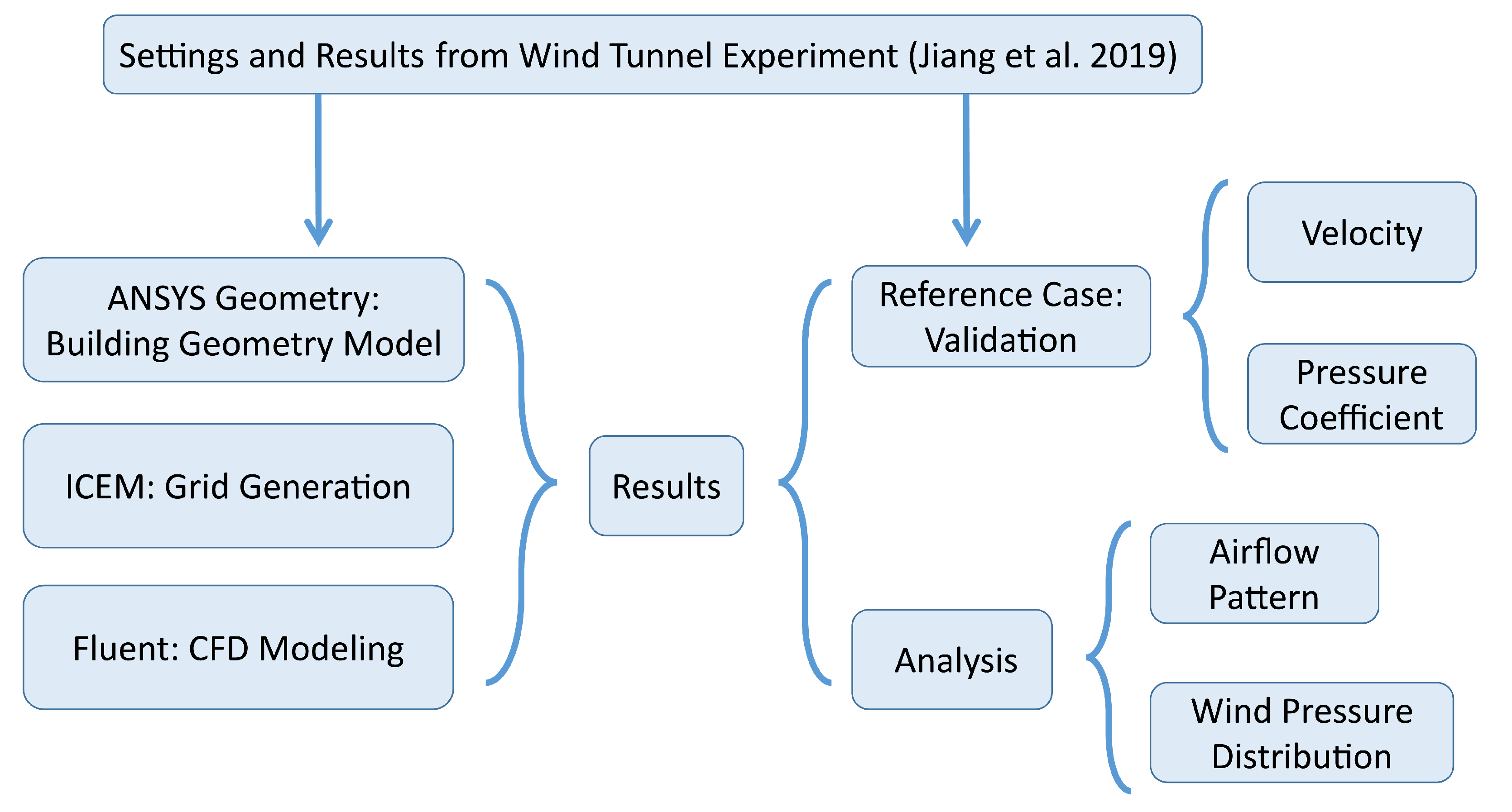
The airflow field around the cube building was experimentally measured at a scale of 1:30 with or without shading louvers by Jiang et al. [44]. The wind tunnel test section was 12 m × 1.8 m × 1.8 m, and the blocking ratio is below 8%. The scales of the test building were 0.5 m for all building edges, and 26 rows of single-sided sunshade louvers were installed near the windward surface. There were five blinds in each row. The slat size was 93 mm (length) × 17.5 mm (width) × 1.0 mm (thickness), and the spacing between adjacent rows was 18.3 mm. The rotation angle of the shading louvers was 45°, and the windward surface was normal to the approaching airflow. The geometric model of the single-shaded building is shown in Figure 2. All louvers have the same rotation angle θ. In Figure 2, W is taken as 0.025 m, and B is taken as 0.0175 m.
The wind velocity was measured on the mid-surface of the wind tunnel for validation, as shown in Figure 3. Some solid elements were set on the ground to establish the atmospheric boundary layer near the inlet of the wind tunnel. The turbulent intensity I and the wind velocity U profiles for the approaching airflow were measured in the wind tunnel. The power law of velocity profile on the inlet is described in Equation (1),
U ( z ) = U ref ( z h 0 ) α
where U(z) is the wind velocity at height z. The reference velocity Uref and the reference height h0 are equal to those experimental parameters, set by Jiang et al. [44] to establish the wind environment in the computational domain. The reference velocity Uref was 3.41 m/s at h0 from the measurement result. The reference height h0 is the building height. α is the coefficient for power-law profile to describe the characteristics of surface roughness considering terrain category and was set as 0.27 for suburban terrain. Figure 4 shows the turbulent intensity I and the wind velocity U profiles of airflow on the inlet of experiments and simulation.

3. CFD Simulation

To evaluate the influence of rotation angle θ of shading louvers on the distribution of wind pressure coefficient in a wider range, six simulation cases with θ = 0°, 15°, 30°, 45°, 60° and 75° were established. The reference case with θ = 45° was applied to validate the simulation results. Figure 5 summaries the numerical process to investigating airflow fields of the shaded building in this study.

3.1. Reference Case

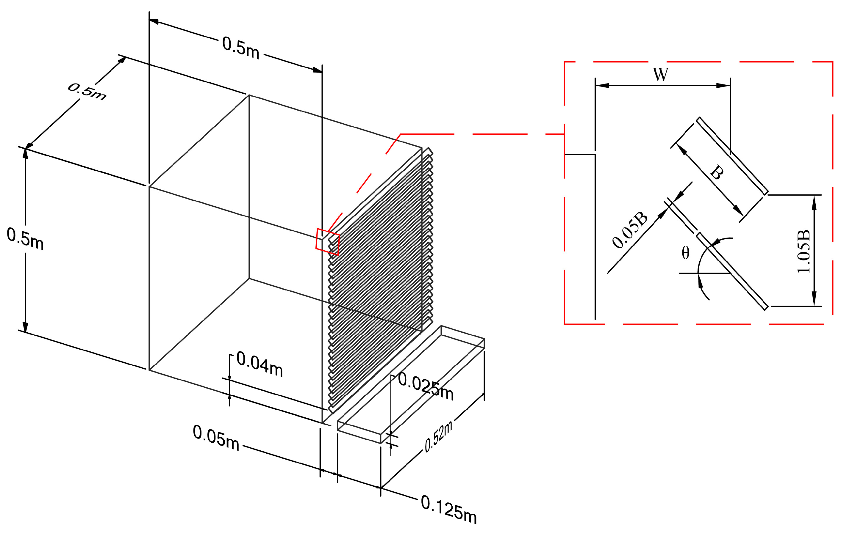
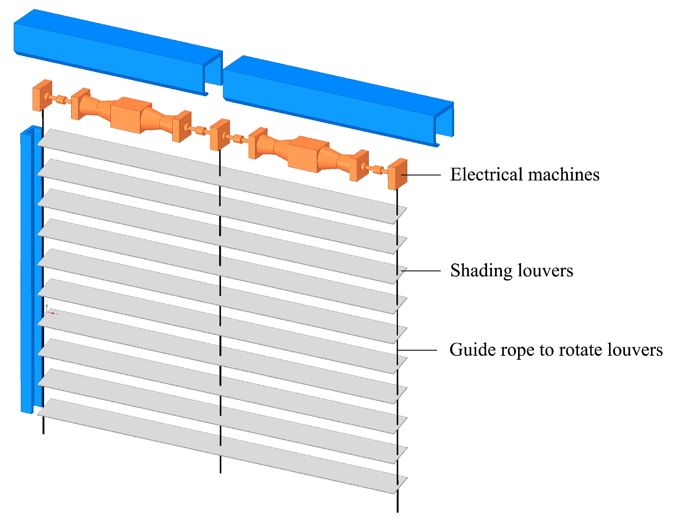
3.1.1. Geometric Model

All scales of the cubic building and single-shaded louvers are the same as those of the building geometry in the wind tunnel experiment, as shown in Figure 2. The geometric settings for two adjacent louvers are described.

3.1.2. Turbulence Model

To investigate the airflow fields around buildings through CFD technology, the two-equation Reynolds-averaged Navier-Stokes models (RANS) were frequently applied as these models have a good balance between accuracy and computational consumption [46,47]. The most widely validated RANS model in urban environment is k-ε turbulence model [48]. For k-ε models, it is not necessary to investigate the turbulent fluctuations thoroughly when simulation is performed for wind characteristics [17,44]. The Reynolds-averaged and time-averaged properties of airflow have sufficient accuracy to perform the simulation around shaded buildings. One of the most commonly used RANS models for urban climates is the standard k-ε model [49]. In addition, some modified k-ε models, like RNG k-ε model and realizable k-ε model, can provide more accurate data for some situations because of their better reproduction of swirling flows [44]. The realizable k-ε model was used in the reference case according to the simulation performed by Jiang et al. [44]. Some other CFD studies of wind pressure coefficient on building surfaces show that k-ε models, especially realizable k-ε model, have good performances at various angles of attack on buildings. For example, Montazeri and Blocken investigated the wind pressure coefficient on a building with balconies by using five turbulence models [17]. The results show that the wind pressure coefficient, obtained from the realizable k-ε model, has good agreement with experimental data. Meng et al. [50] investigated wind pressure coefficient on a high-rise building at different angles of attack and by using five turbulence models. The results show that realizable k-ε model has good performances at angle of attack from 0° to 90°.

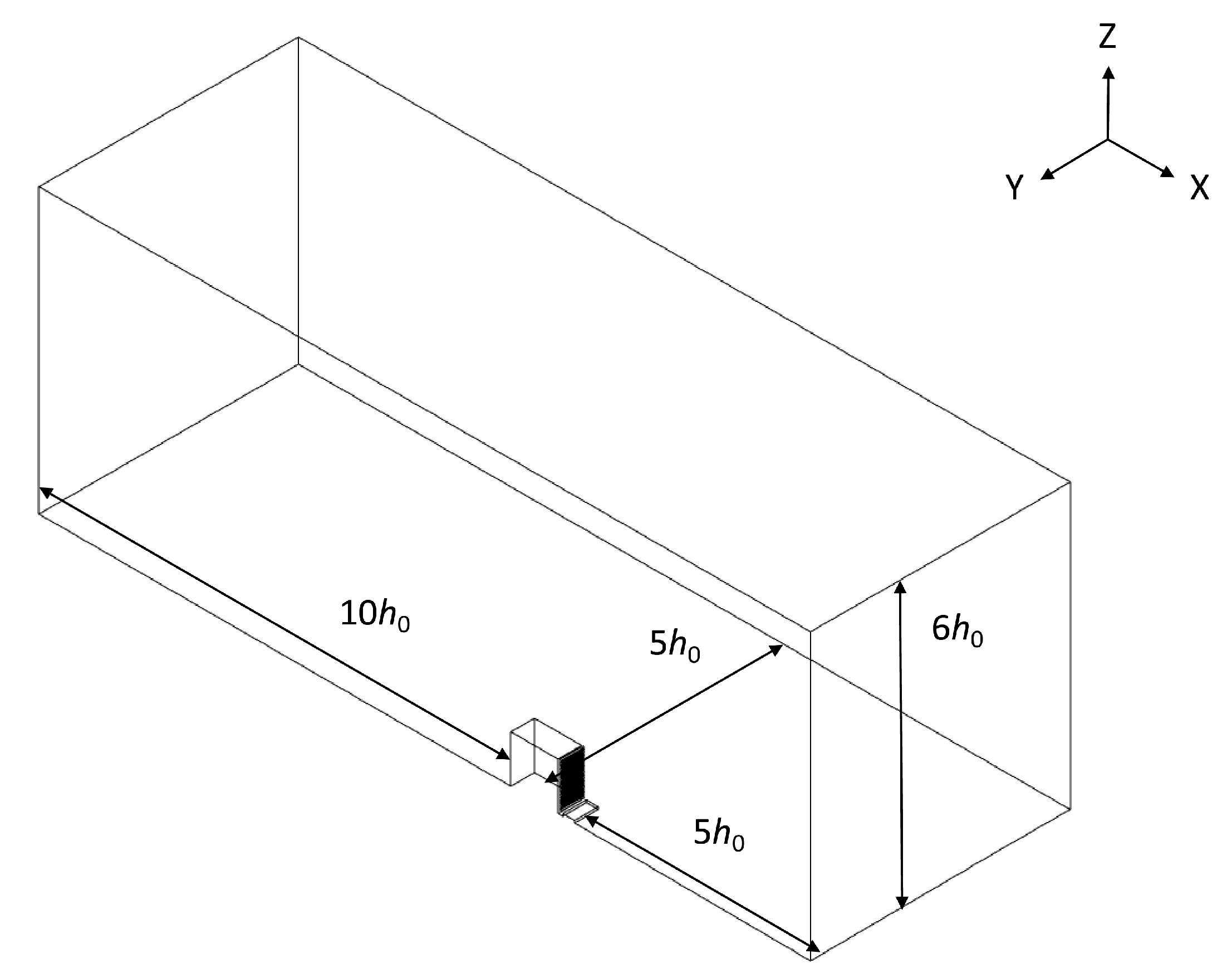
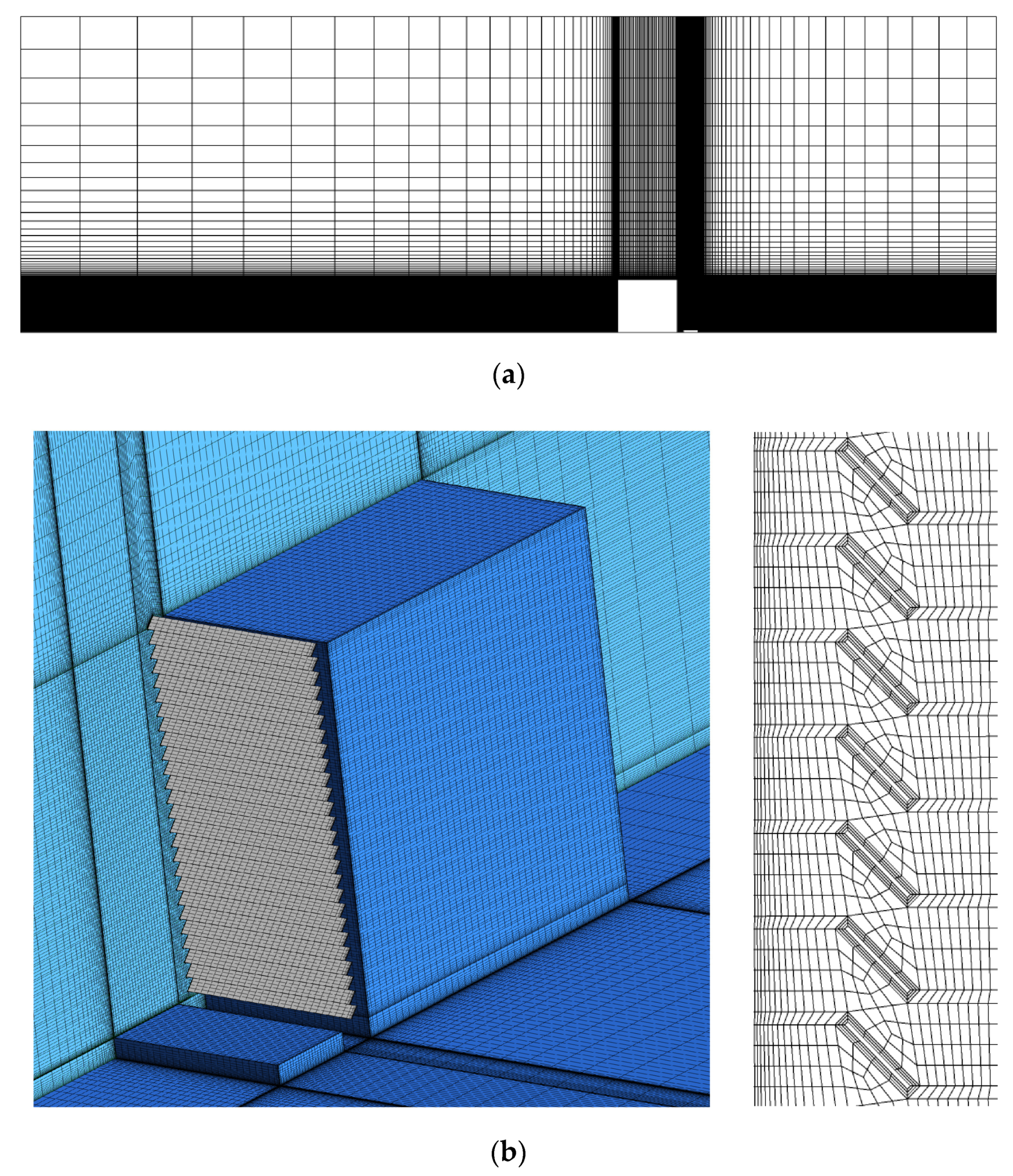
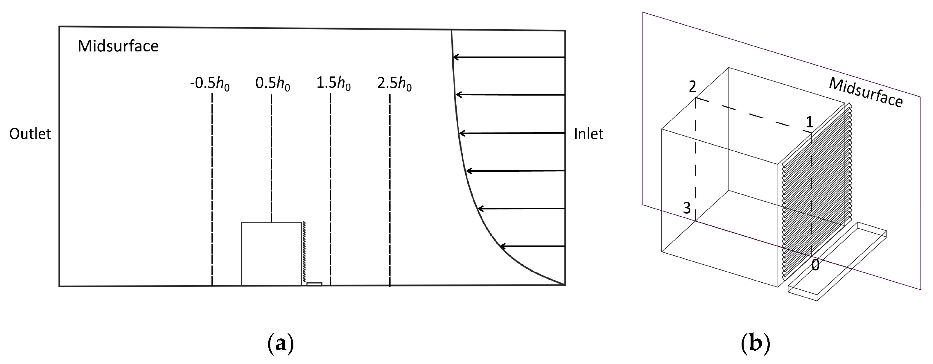
3.1.3. Computational Domain and Grid Resolution

The computational domain around the studied building is demonstrated in Figure 6. Two standards were used to define the scales of the computational domain [46,47], and the blockage ratio is below 3%. The minimum heights of the near-wall grids on the ground, building walls and shading louvers were 0.0003 m (0.0006h0). Note that the near-wall grids are just the wall-adjacent grids closed to the solids, rather than all grids between two adjacent louvers. In near-wall boundary layers on these surfaces, enhanced wall treatment is applied for y+ < 5 and y+ ≈ 1 [51]. Figure 7 shows the grid resolution in computational domain and around the cubic building. Compared with published research of a building with louvered windows [12], we had much higher grid density along louver length but lower grid density along louver width, because in our pre-simulation, it was found that in the study of wind pressure coefficient, the deviations were mainly caused by the grid density along louver length, rather than that along louver width. Based on the grid resolution, a coarser mesh and a finer mesh were created to ensure grid accuracy. The Grid Convergence Index (GCI) [52,53] was calculated to show the deviation between different mesh sizes. For the reference case, GCI of normalized velocity and wind pressure coefficient are 0.37% and 1.8%, which are small enough to ensure grid accuracy, as recommended by Vinchurkar and Longest [54].

3.1.4. Boundary Conditions

In the reference case, the airflow inlet in front of the louvers was defined as velocity inlet. The turbulent intensity I and wind velocity U of the approaching airflow given by Equation (2) and Equation (1) are measured in the wind tunnel experiment by Jiang et al. [44] and applied, in order to calculate the turbulent kinetic energy k and turbulence dissipation rate ε by using Equations (3) and (4):
I ( z ) = 0.1 ( z h 0 ) a 0.05
k ( z ) = [ U ( z ) I ( z ) ] 2
ε ( z ) = C μ 0.5 k ( z ) U ( z ) h 0 α ( z h 0 ) α 1
The measurement results of velocity U and turbulent intensity I on the inlet obtained from the experiments and their fitting profiles for CFD simulations are shown in Figure 4. The constant value Cμ is set as 0.09 [47].
On the louvers, ground and building surfaces, the boundary conditions were defined as no-slip wall, on which the fluid sticks to the solid plane. For all these wall boundaries, enhanced wall treatment was used to simulate the near-wall airflow with y+ < 5. The top and the lateral boundaries were defined as symmetry, which means that the normal velocity and normal gradients of all variables are taken as zero at this boundary. The outlet was defined as outflow, on which the diffusion fluxes are zero for all flow variables [51].

3.1.5. Solver Settings

The discretized governing equations were solved by the finite volume method (FVM) in the steady state. The SIMPLEC algorithm was applied to couple the pressure and momentum equations. The second-order upwind difference scheme was applied for discretizing turbulent kinetic energy, momentum and turbulent dissipation rate. When the scaled residuals were below 10−6 for x, y, z momentum and 10−4 for continuity, k and ε, the convergence of the simulation was considered to be achieved. The monitors were also set at some points in the measurement lines in the simulation to verify the convergence. Oscillatory convergence was observed for the scaled residuals. As recommended by Ref [34] and [55], the results were monitored for more than 10,000 iterations. There were no significant oscillations in measurement lines of velocity and pressure, the average values over the last iterations were unnecessary and not calculated.

3.1.6. Calculation of Wind Pressure Coefficient

Wind pressure coefficient Cp is calculated from the pressure difference between static pressure P on the building surfaces and static pressure Pref at the reference point, as provided in Equation (5):
C p = P P ref 1 2 ρ U ref 2
The reference point was set on the lateral boundary at the reference height h0 and had the same distance from the inlet to the windward facade. ρ is the air density and taken as 1.225 kg/m3.

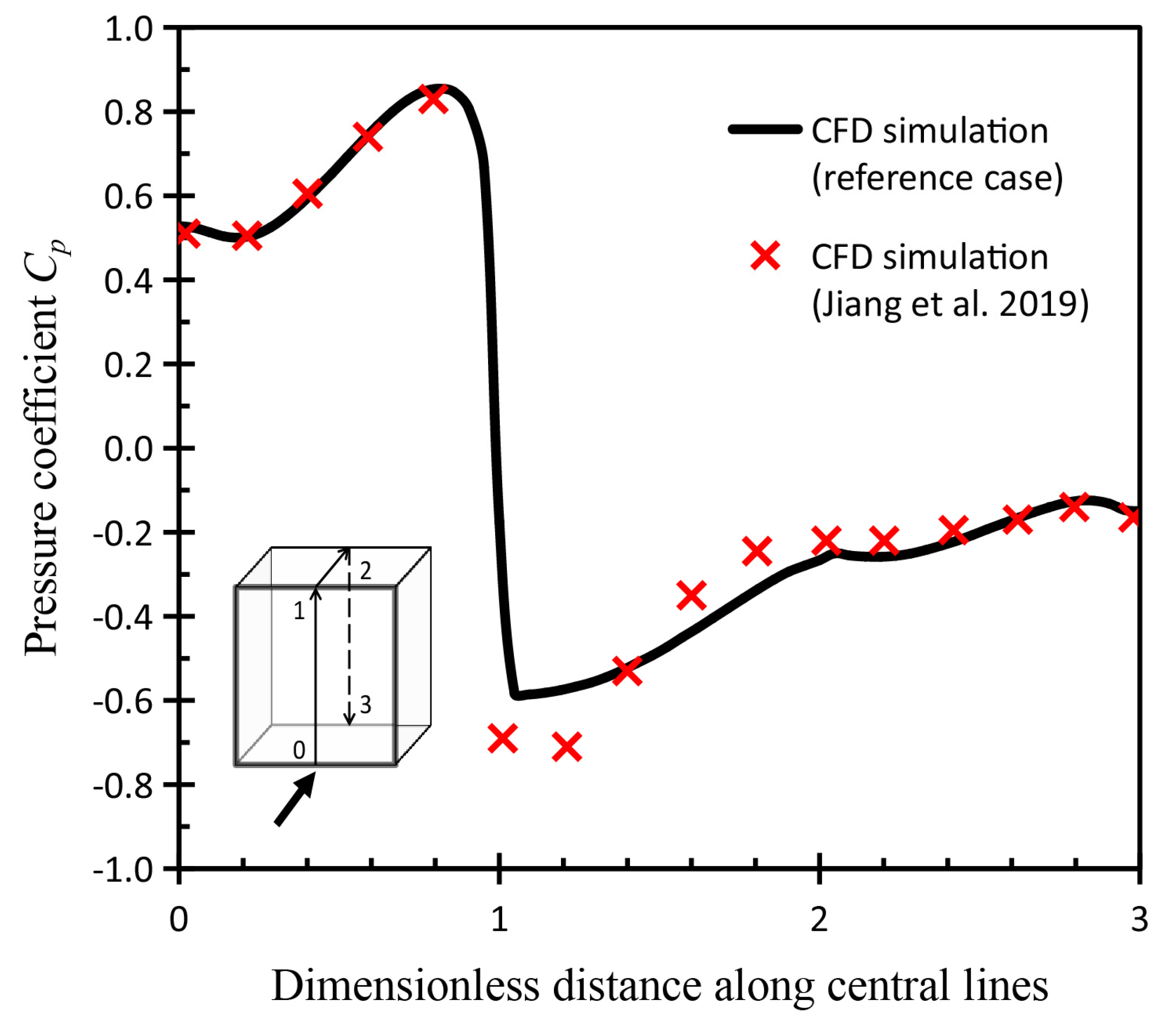
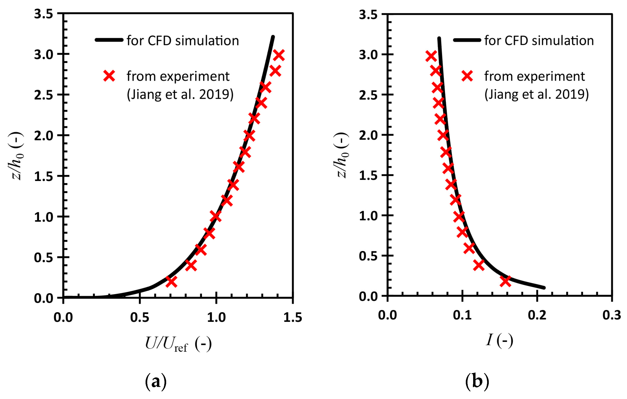
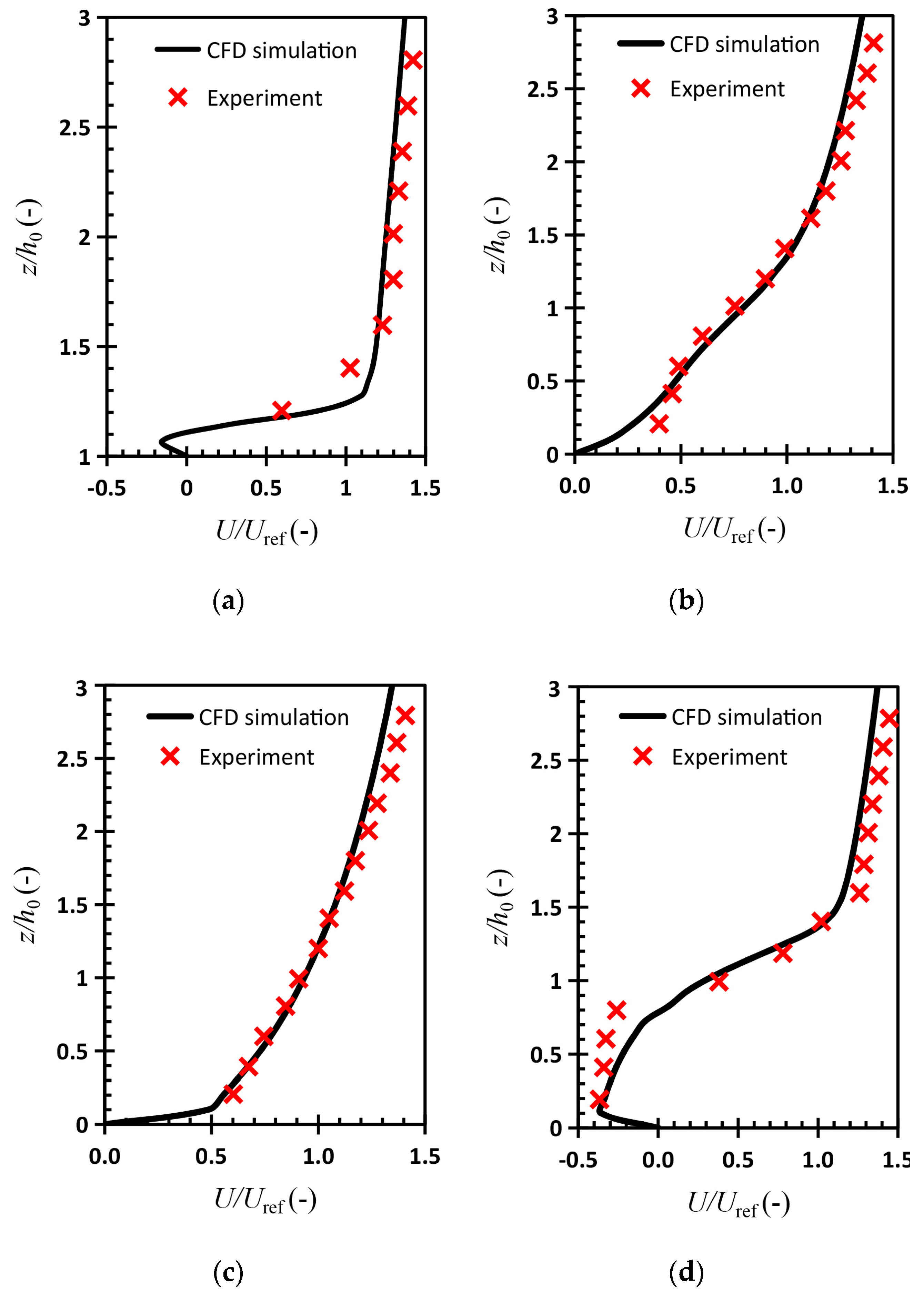
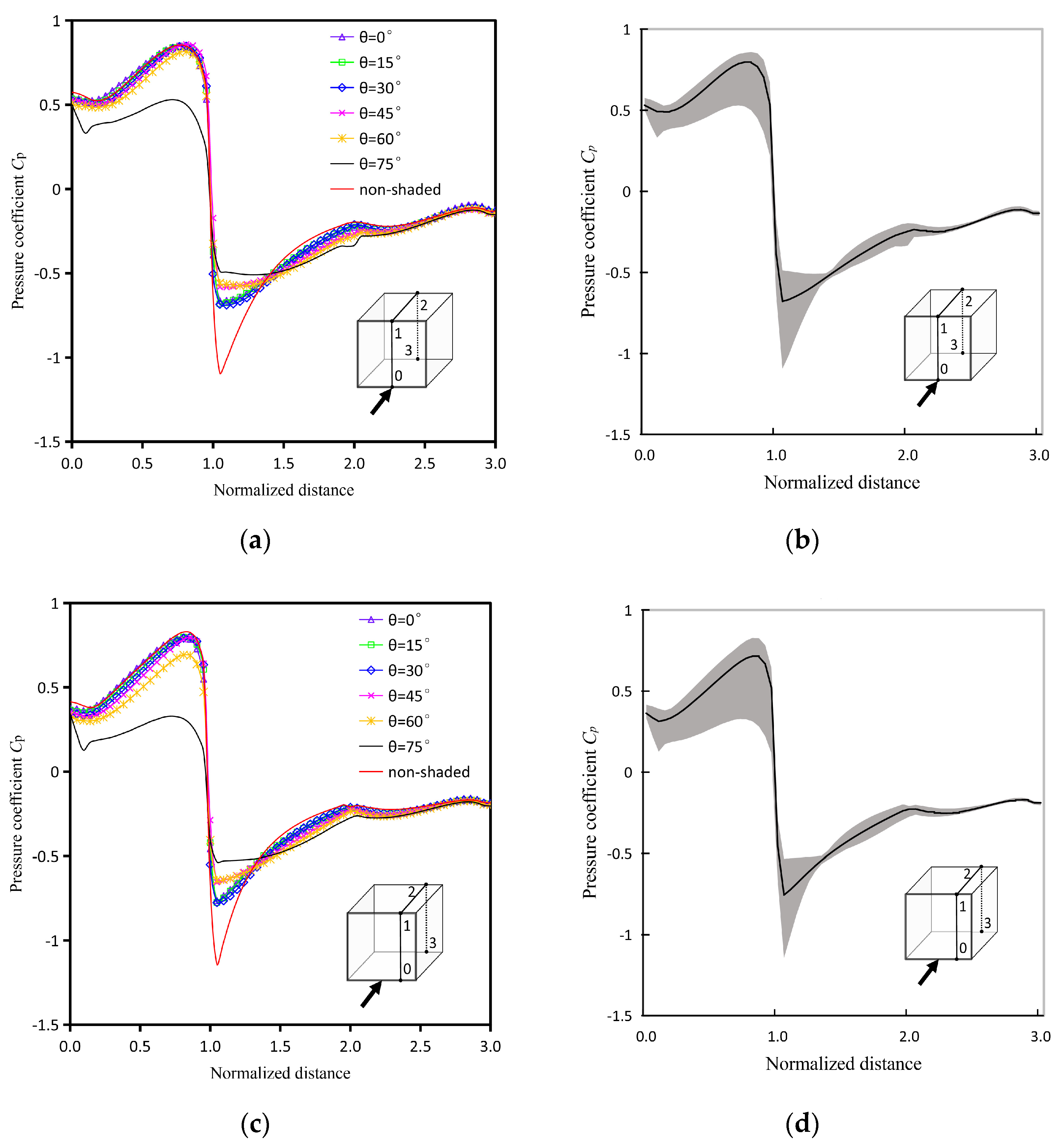
3.2. Result Validation

Validation was performed by comparing the deviation between the numerical results of the reference case and the experimental data from Jiang et al. [44]. In that reference, research with experimental and numerical results, allowed the velocity value to be measured at some points along several lines, which was on the mid-surface of the cubic building and perpendicular to the ground in the wind tunnel, while wind pressure coefficients were investigated along three lines on the intersection between building surfaces and the mid-surface in CFD simulations. The normalized velocity Un as shown in Equation (6) is to demonstrate the airflow velocity distribution:
U n ( z ) = U ( z ) U ref
Figure 2 demonstrates the measurement locations to validate the numerical results. Figure 8 shows the normalized velocity U/Uref distribution of the simulation data and the experimental results on vertical measurement locations. The average absolute deviation is 0.068 between simulation data and experimental data. Figure 9 shows Cp distribution for comparison of the data from the reference case and the data from Jiang et al. [44] along measurement lines on the windward, roof and leeward surfaces. The average absolute deviation is 0.046 between the two cases for wind pressure coefficient. The average values of U/Uref and Cp, as long as their deviation on each line, are shown in Table 1. The comparison results show that U and Cp in the reference case are in good agreement with results from the previous study. The U and Cp tendencies on these locations can be reproduced well by CFD technology. The maximum deviations occur beyond the roof for both, U and Cp distributions. This phenomenon seems to be that the realizable k-ε model with default parameters may provide airflow characteristics with overestimated reattachment lengths on the roof, and in the recirculating region at the corner between the ground and the leeward facade [32,56,57]. This over-estimation leads to the U near the roof and leeward facade and the smaller gradient for Cp along the roof line. Although, there are higher distortions in the reattachment region for the realizable k-ε model, the simulation accuracy is considered to be suitable enough to perform CFD simulations.

4. Results and Discussion

When openings are installed on outside surfaces of a sealed building, the pressure distribution on the envelope can be applied to forecast air leakage, design indoor airflow routes and evaluate natural ventilation patterns in different wind environments [17]. Analyzing the distribution of wind pressure coefficient Cp on shaded building surfaces is critical for exploring the potential ventilation capacity. For a sealed building, orifice equation assumes that the pressure distribution is independent to the presence of openings [13]. In orifice equation, Cp is applied to calculate wind-induced airflow rate Q of natural ventilation in buildings [14,15], as shown in Equations (7) and (8),
Q = C d A 2 Δ P ρ
Δ P = 1 2 ρ U ref 2 C p P i
where A is the area of an opening in the sealed building assumption. Cd is the discharge coefficient. Pi is the pressure inside the building.

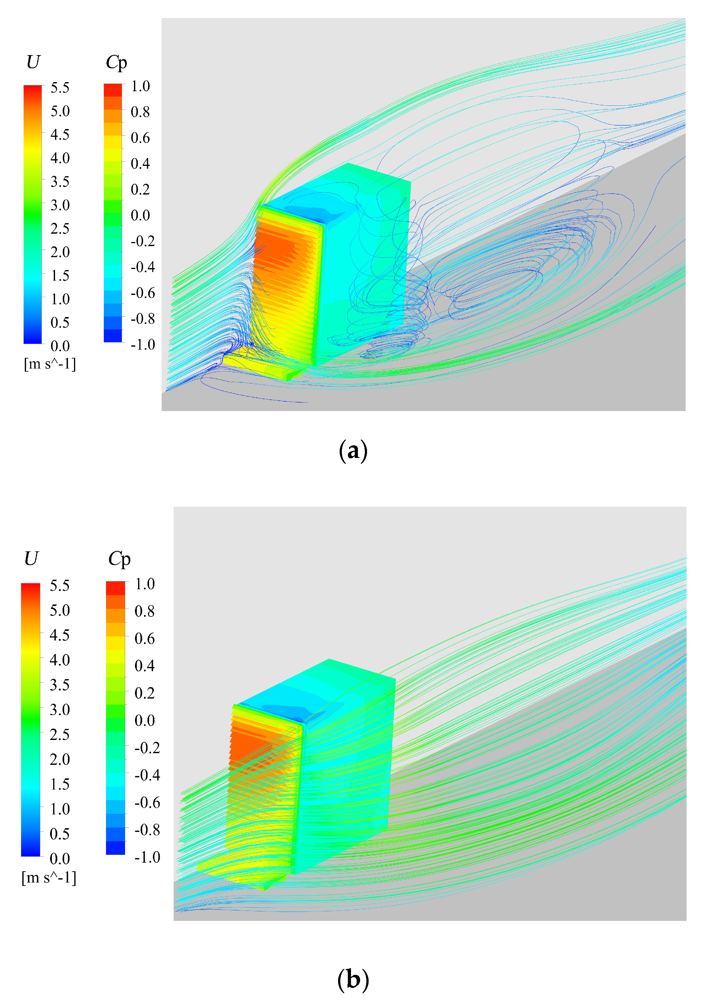
4.1. General Features of Airflow Pattern

Figure 10 shows airflow streamlines around the building and wind pressure distribution on the building surfaces under the shaded condition with θ = 45°. In Figure 10a, the approaching flow towards the central rows was separated into three regions: Stagnation zone on the windward facade at about 0.7h0, the upward flow near the roof and the downward vortex near the ground. The streamlines were smooth above the small reverse flow on the roof. The larger reverse flow and the recirculating zone were generated on the lateral façade, and the leeward facade, respectively. In Figure 10b, the airflow streamlines towards the side rows were smoother than that towards the central rows, which demonstrates that the airflow pattern was almost not affected by the detailed geometry of the shaded building.

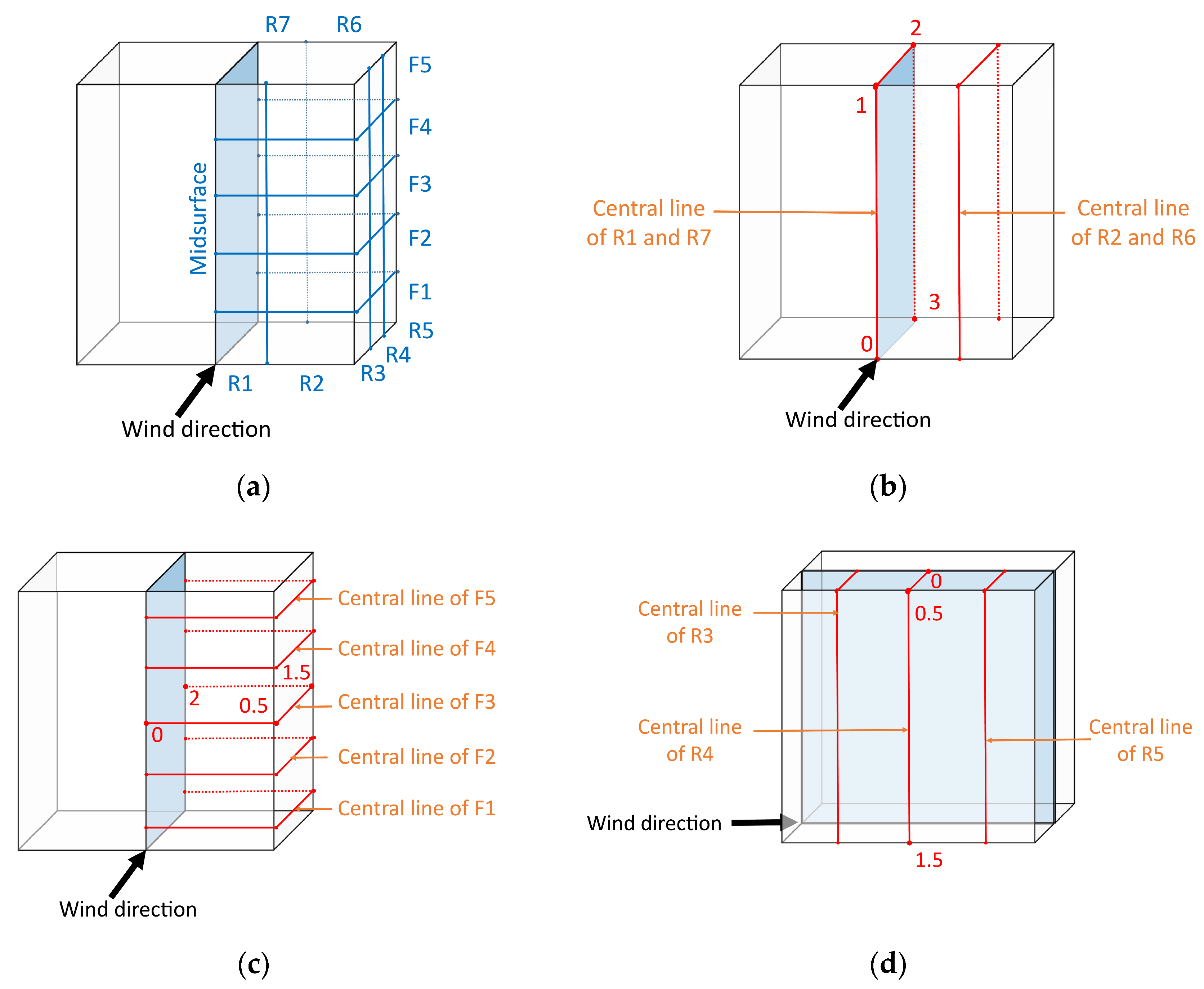
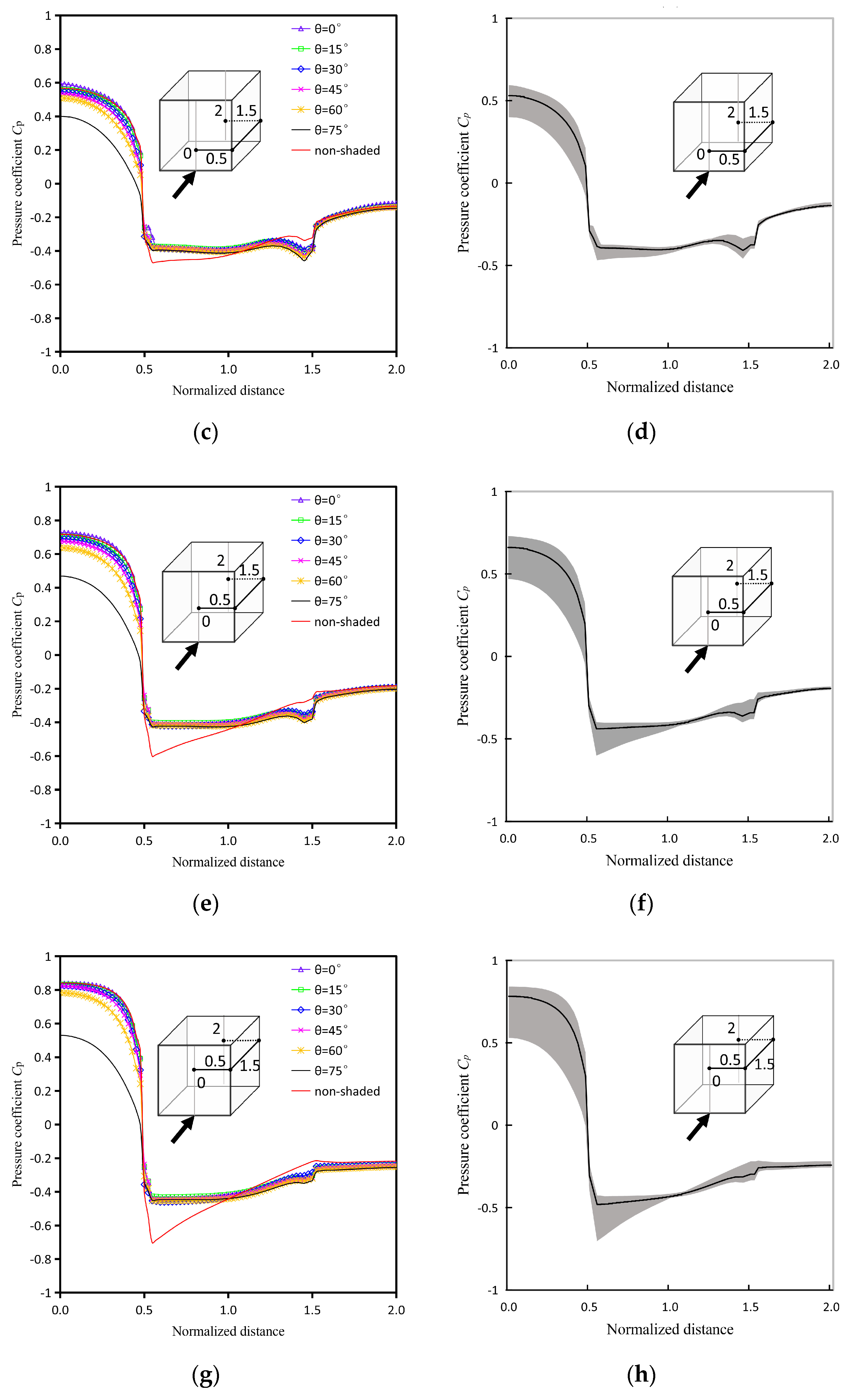
4.2. Features of Local Wind Pressure Coefficient along Measurement Lines

The windward, lateral and leeward facades are divided into seven equal rows and five equal floors to ensure that the outside surfaces of rooms have the same area in the same direction. The rows are marked from R1 to R7, and the floors are marked from F1 to F5, as shown in Figure 11a. Note that the area for calculation is half of the real area for R1 and R7, considering the usage of the symmetry building model and symmetry domain in simulations. The distribution of wind pressure coefficient are investigated on two W-R-L lines, five W-S-L lines and three R-S lines. All these lines are located on the center of their rows or floors, which are also shown in Figure 11b–d. The impact of shading louvers with various rotation angle θ on Cp at a specific point is evaluated by the range R as shown in Equation (9).
R = C p-max C p-min
where R is the range of wind pressure coefficient Cp at a specific point on a measurement line for different shaded conditions. Cp-max and Cp-min are the maximum and minimum Cp at that point in these shaded conditions. Note that Cp-max and Cp-min only represent the local values of a special point on a line in all shaded cases, which are different from the maximum and minimum Cp on a whole line.

4.2.1. Local Wind Pressure Coefficient on W-R-L Lines

Figure 12a,b present the local range R, local and average value of wind pressure coefficient Cp on the central lines of R1 and R7 along the windward, roof and leeward surfaces under different shaded conditions. Generally speaking, the roof suffers the largest fluctuation of Cp, while the leeward surface has the smallest difference of the local Cp and R along the lines. The maximum and minimum value of Cp are 0.86 and −1.08, respectively. The Cp-max line and Cp-min line have the similar shape and tendency except near the edge of the roof for around 1–1.4h0 where has a flow separation. On the line of the windward facade, the maximum R is at about 0.8–0.9h0 on the stagnation zone and the minimum R is near the edge between the windward and the roof surfaces. The R along these lines increases along 0–0.1h0, but the local Cp decreases. From 0.1h0 to 0.7h0, the local Cp and the R both increase. After 0.7h0, the local Cp in some cases begins to decrease but the R still grows up until around 0.9h0. These results indicate that near the maximum positive Cp on the stagnation zone, the Cp is strongly sensitive to the rotation angle θ of shading louvers. For the area near the vortex at the corner of the windward facade and the ground, the Cp is not sensitive to different shaded conditions. On the lines of the roof, the Cp suffers a sharp decrease near the edge, which is the continuation of the windward surface. Then the R increases to the widest at 1.05h0. In this area, the blocking effect of shading louvers makes the Cp tendency smoother along the roof line. On the leeward line, the local Cp just changes slightly at different points due to the leeward recirculation.
Figure 12c,d present the local range R, local and average value of wind pressure coefficient Cp on the central lines of R2 and R6 along the windward, roof and leeward surfaces. Generally speaking, the tendencies of the Cp-max line and the Cp-min line along the lines in Figure 12d are similar to those in Figure 12b. The R along the central lines of R2 and R6 is smaller than that along the central lines of R1 and R7. However, there are also some significant differences between the two locations. On the windward surface, the R along the central lines of R2 is always larger. Even if the maximum Cp on two locations are almost the same, the local Cp-min near the ground is obviously different between two locations. the Cp-max along the central lines of R1 is over 0.5 within 0–0.9h0, but the Cp-max along the central lines of R2 is below 0.5 within 0–0.3h0. The shape difference on the Cp-min line is not as obvious as that on the Cp-max line. The Cp-min along the central lines of R2 is about 0.2 smaller. These differences mean that on the lines of R2, the windward surface tends to suffer a larger fluctuation of positive wind pressure. On the roof, the shape and tendency of the Cp-max and Cp-min on the central lines of R2 and R6 are almost the same as those on the central lines of R1 and R7, and only the R is a little smaller for most locations than the central line. On the leeward, the gradient and the maximum value of Cp along the central lines of R6 are slightly lower than those along the central lines of R7.

4.2.2. Local Wind Pressure Coefficient on W-S-L Lines

Figure 13a,b present the local range R, local and average value of wind pressure coefficient Cp on the central lines of the first floor along the windward, the lateral and the leeward surfaces. The windward surface suffers the largest fluctuation of Cp, while the lateral wall has the smallest fluctuation of Cp. Generally speaking, the windward surface has the widest R and the largest difference of the local Cp along the central line. The leeward surface has the smallest R along the central lines. The Cp-max line and the Cp-min line have the similar shape and tendency. The maximum value and the Cp-min are 0.55, and −0.44, respectively. On the windward surface, the largest R locates at 0.38h0 and the smaller R locates on the edge between the windward and the lateral surfaces. On the lateral surface, the R increases slightly along 0.5–0.8h0, then within 0.8–1.2h0 the R are almost the same. From 1.2h0 to 1.4h0, the R increases obviously, then it decreases again near the edge between the lateral surface and the leeward surface. On the leeward surface, the local Cp increases obviously but the R just increases slightly.
Figure 13c–j present the local range R, local and average value of wind pressure coefficient Cp on the central lines of the F2–F5 along the windward, the lateral and the leeward surfaces. Generally speaking, the tendencies of the Cp-max and Cp-min along the central lines on different floors are similar to those on F1. The maximum value on the Cp-max line is larger when the floor is higher, except for F5, on which the maximum value on the Cp-max line is a little smaller than those on F4. The minimum value on the Cp-min line is lower when the floor is higher. The locations of the minimum value on the Cp-min lines are on the lateral surface for all floors. However, for F1 and F2, the locations are near edge of the windward surface at around 1.4h0, while for the higher floors, Cp near the edge of the leeward surface at around 0.55h0 is the minimum value on the Cp-min lines. On the windward surface, the R along the central lines is wider for the higher floors. The absolute gradient of the Cp-max line becomes lower near the central vertical lines but becomes higher near the edge of the lateral surface. On the lateral surface, the R becomes wider at around 0.55h0 for the higher floors because of the lower Cp-min. Along the lines on the lateral surface, the location of the minimum R becomes closer to the windward surface, as the floor becomes higher. The fluctuation of R near the edge of the leeward surface becomes smooth. This phenomenon means that as the floor gets higher, the wind suction effect of reverse flow becomes greater than the effect of the backward recirculation, but the negative pressure area, caused by the reverse flow, seems to be smaller than the negative pressure area caused by recirculation. On the leeward surface, the R along the central lines are similar for F1, F2 and F3, while the R are a little wider for F4 and F5. The absolute gradient of Cp becomes lower for the higher floors, which means that higher floors are prone to have smoother Cp distribution along these lines.

4.2.3. Local Wind Pressure Coefficient on R-S Lines

Figure 14a–f presents the local range R, local and average value of wind pressure coefficient Cp, on the central lines of R3–R5, along the roof and leeward surfaces. The Cp distributions along R-S lines are obviously smoother than Cp along W-R-L and W-S-L lines, because only the windward surface undergoes positive wind pressure. Generally, The R has the largest value on the central lines of R3, while R has the smallest value on the central lines of R4. The result indicates that R4 on the lateral surface seems to be the transitional zone, where the impact of reverse flow becomes weaker, so the presence of shading louvers cannot change Cp greatly. On the three lines, most local R on the roof is larger than those on the lateral surface. The maximum Cp locates on the lateral surface near the ground for the central lines of R3 but on the roof for the central lines of R4 and R5. The minimum Cp locates on the roof for the central lines of R3 and R4 and on the lateral surface for the central lines of R5. The largest R locates at 0h0 for the central lines of R3 and R5 and at around 0.48h0 near the edge between the roof and lateral surfaces for the central lines of R4. The R changes strongly along the central lines of R3 but more slightly along other two lines. The result of R3 means that the reverse flow near the roof and the lateral surface are both sensitive to the shaded conditions.

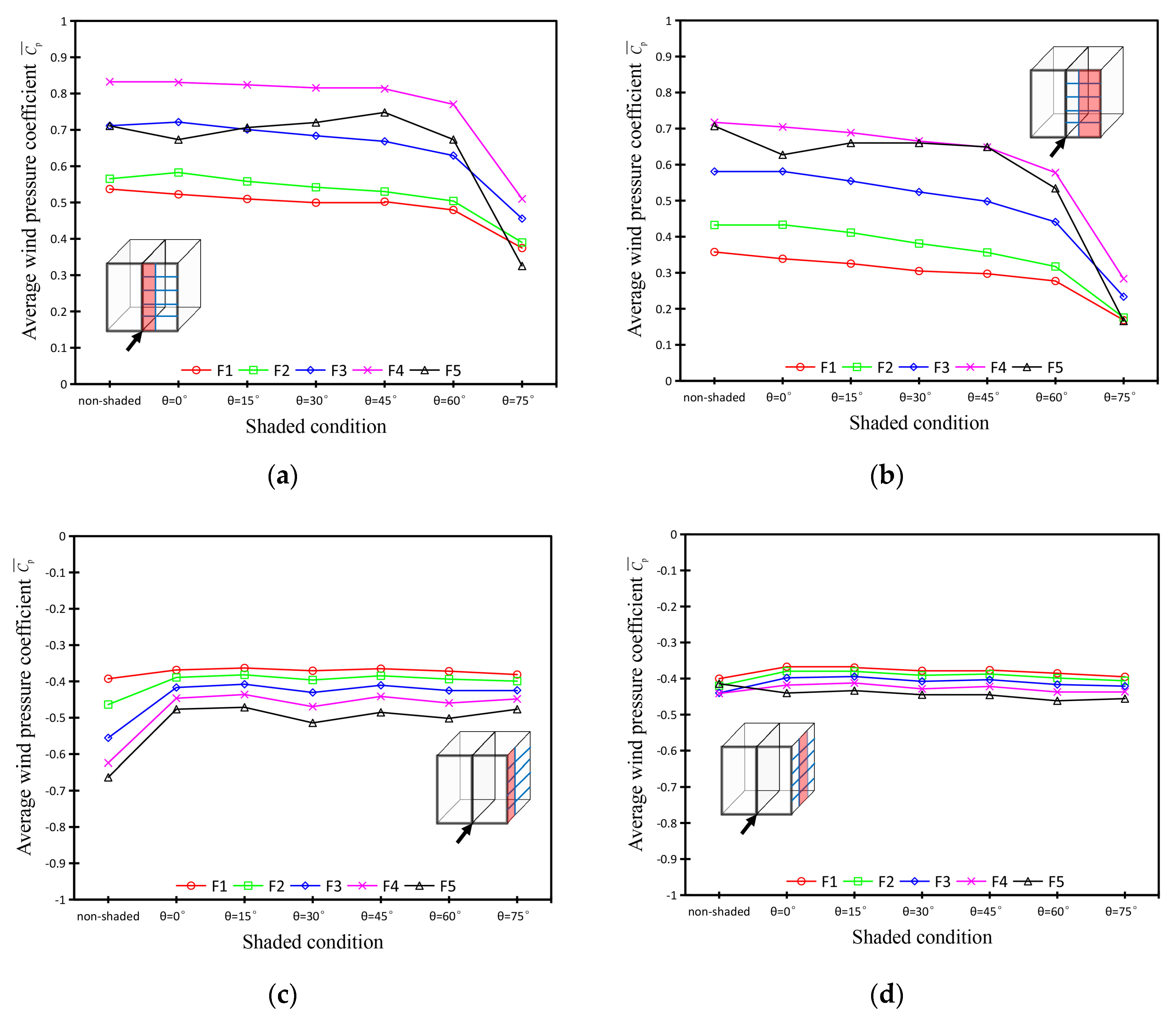
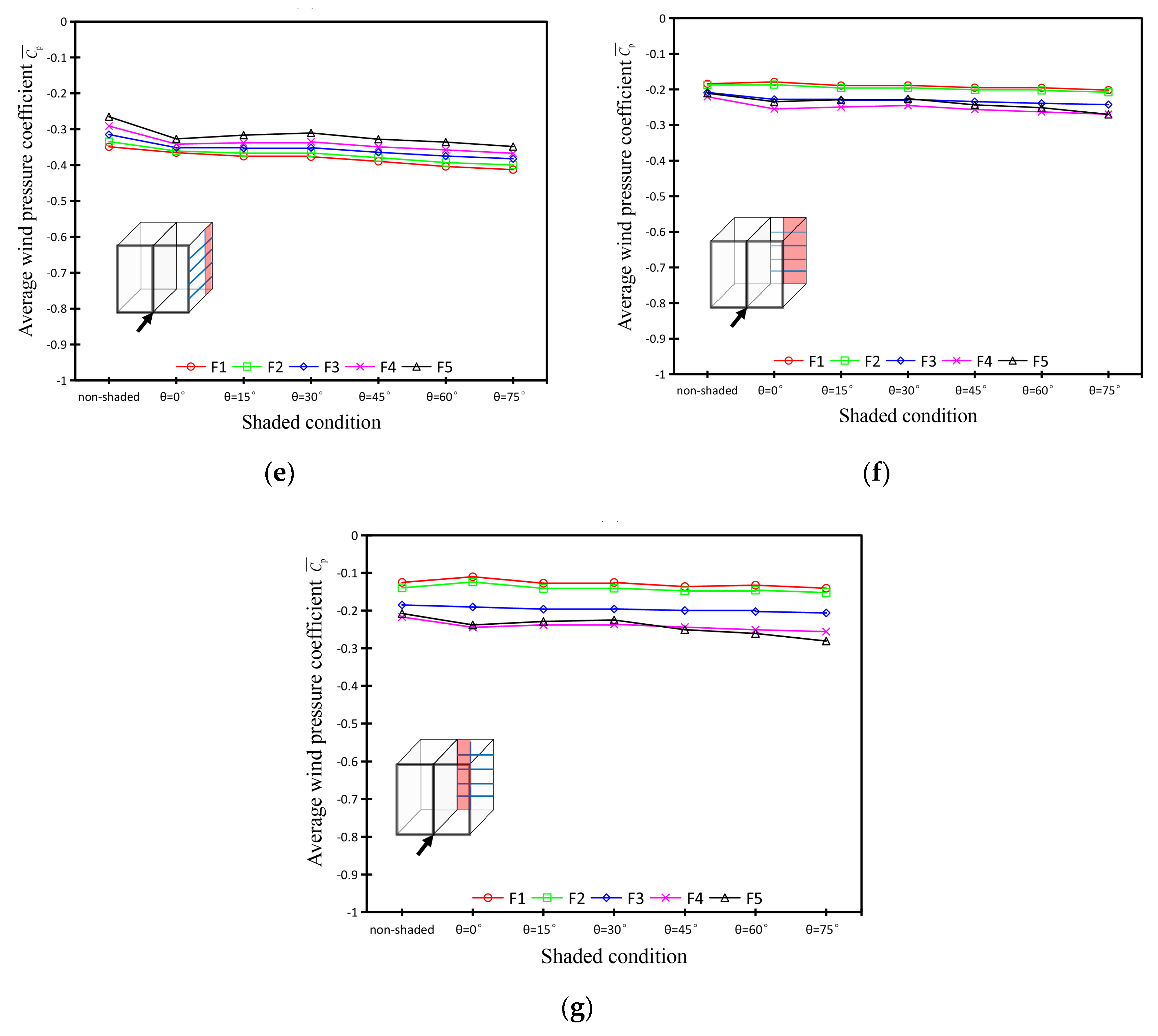
4.3. Impact of Shading Louvers on Average Wind Pressure Coefficient

Some parameters are introduced to describe the characteristics of average Cp on outside surfaces of rooms. C p ¯ is the average Cp on outside surface of a room belongs to the intersection of one floor and one row, as given by Equation (10). Δ C p ¯ is the difference of C p ¯ between a shaded condition and the non-shaded condition, as given by Equation (11). Δ C p - R ¯ is the average difference of C p ¯ for all shaded conditions, compared with the non-shaded condition in a special row, as given by Equation (12). Δ C p - θ ¯ is the average difference of C p ¯ between a specific shaded condition and the non-shaded condition in a whole row, as given by Equation (13),
C p ¯ = 1 A R A R C p   Δ S R
Δ C p ¯ = C p ¯ C p - n ¯
Δ C p - R ¯ = i = 1 6 | C p - θ - i ¯ C p - n ¯ |
Δ C p - θ ¯ = j = 1 7 | C p - R - j ¯ C p - n ¯ |
where AR is the area of the outside surface of a room. In all simulation cases, the rooms in different floors and rows are assumed to have the same AR. Considering the usage of the symmetry model and symmetry domain in simulations, AR in R1 and R7 are set as the half value of the real area. ∆SR is the area of a grid on the outside surface. C p - θ - i ¯ is the C p ¯ for the shaded condition with a specific rotation angle θ, and i is set as 1–6 to represent θ = 0°, 15°, 30°, 45°, 60° and 75°. C p - n ¯ is the C p ¯ in the non-shaded condition. C p - R - j ¯ is the C p ¯ in a specific row, and j is set as 1–7 to represent R1–R7.
Figure 15 presents C p ¯ on five different floors along R1–R7. Figure 16 presents Δ C p ¯ between the non-shaded condition and other shaded conditions. In Figure 15, the C p ¯ results of R1 and R2 show that the windward surface has the largest difference of C p ¯ on different floors for most shaded conditions. On the windward R1 and R2, F4 has the highest C p ¯ and F1 has the lowest C p ¯ for most shaded conditions. C p ¯ has the greatest reduction for all floors when θ turns from 60° to 75°. For most floors, C p ¯ decreases with a higher θ, except for F5. On the lateral R3, the greatest difference occurs between the non-shaded condition and the shaded condition for any θ, but C p ¯ does not have much fluctuation when θ changes. The C p ¯ results of R4, R5 and R6 show that the smallest difference of C p ¯ for different floors occurs near the edge between the lateral and leeward surfaces. The results of R4, R5, R6 and R7 show that the impact of shading louvers on C p ¯ can be neglected in some non-shaded facades. In Figure 16, the impact of shading louvers on C p ¯ , which is described as Δ C p ¯ , becomes higher for the higher floors in general. Considering the different rows, R2 and R3 have the largest and the second largest Δ C p - R ¯ for most floors with the presence of shading louvers. And the impact of shading louvers on C p ¯ is obviously smaller for R4, R6 and R7. With shading louvers, C p ¯ on R3 are larger than those without shading louvers for all floors. And the situation are almost the same on R4 except for F5. But on the most parts of other rows, C p ¯ decreases when shading louvers are installed. For F1, the largest and the second largest Δ C p - R ¯ occur on R1 and R2. The largest absolute value of Δ C p ¯ occurs on R4 for just θ = 0° and on R2 for the other θ. For F2 to F5, the largest and the second largest Δ C p - R ¯ occur on R2 and R3. The presence of shading louvers has the largest influence on Δ C p ¯ of R3 for θ = 0°–45° but on Δ C p ¯ of R2 for higher θ.

5. Conclusions

Taking into account rotation angle of shading louvers, this study investigated the distribution of wind pressure coefficient of a multi-storey building, with single-shaded louvers, through CFD simulation, in order to analyse the potential ventilation capacity of the shaded building. A comparison for validation was performed between the numerical results and data from the previous study. To investigate the wind pressure distribution in detail, the studied outside surfaces were divided into seven rows and five floors to obtain the average wind pressure coefficients of different rooms. The local wind pressure coefficients were also measured along central lines of different rows and floors. The rotation angle of louvers was taken as 0°, 15°, 30°, 45°, 60° and 75°. Through the analysis of the impact of shading louvers, some conclusions are provided as follows:
  • The validation of the studied building shows a small deviation between the numerical data and the data from the previous study. The average absolute deviation is 0.046 for wind pressure coefficient Cp and 0.068 for normalized velocity U/Uref. The Grid Convergence Index of U/Uref and Cp for the reference case is 0.37%, and 1.8%, respectively. Therefore, the parameters of the simulation cases are feasible for the shaded building, and the computational settings is useful for further case studies of shaded buildings.
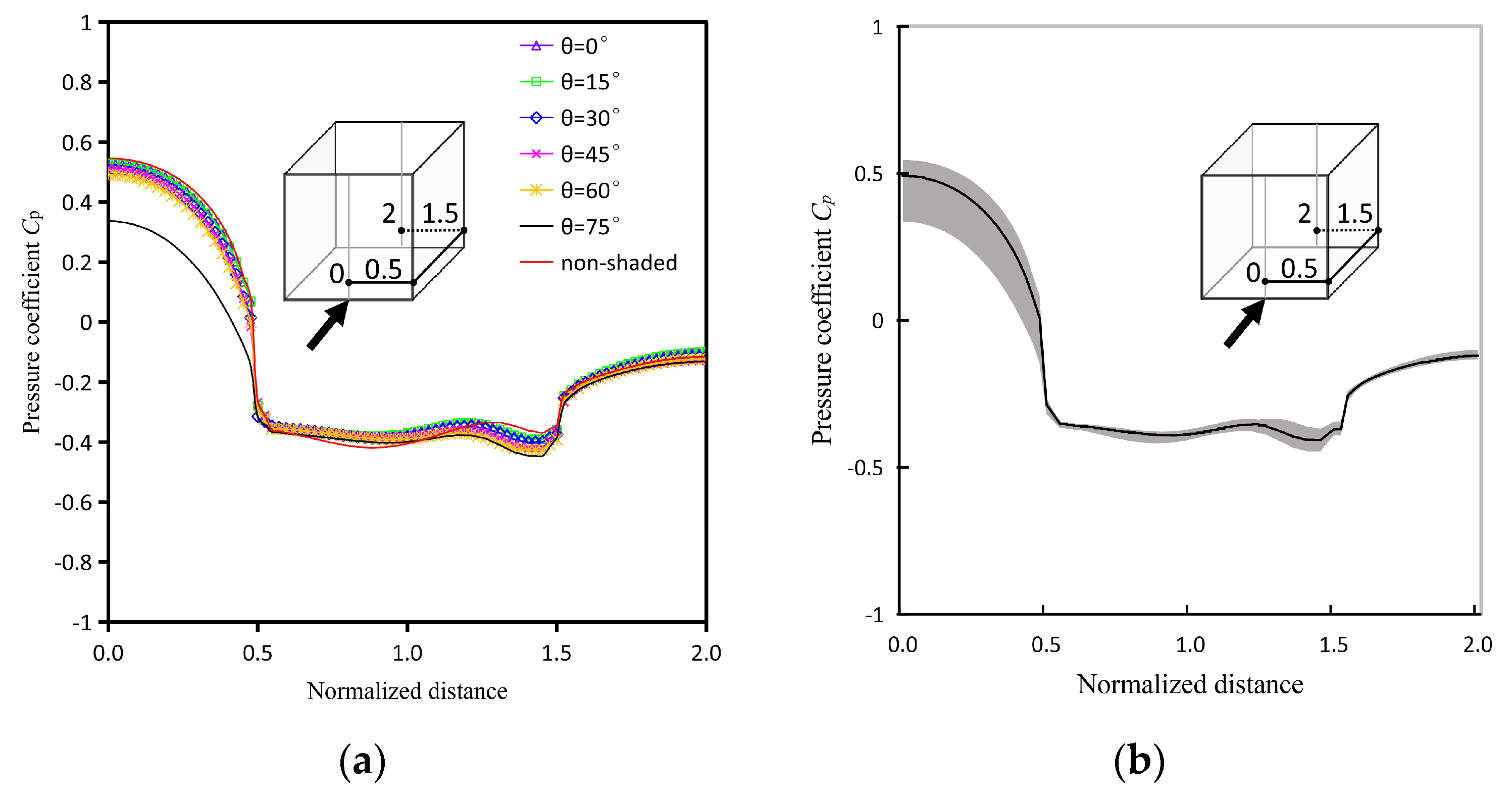
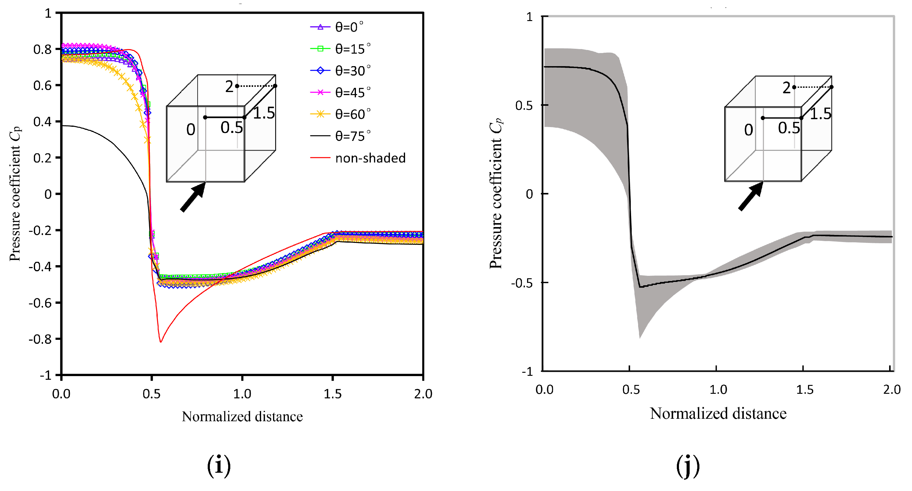
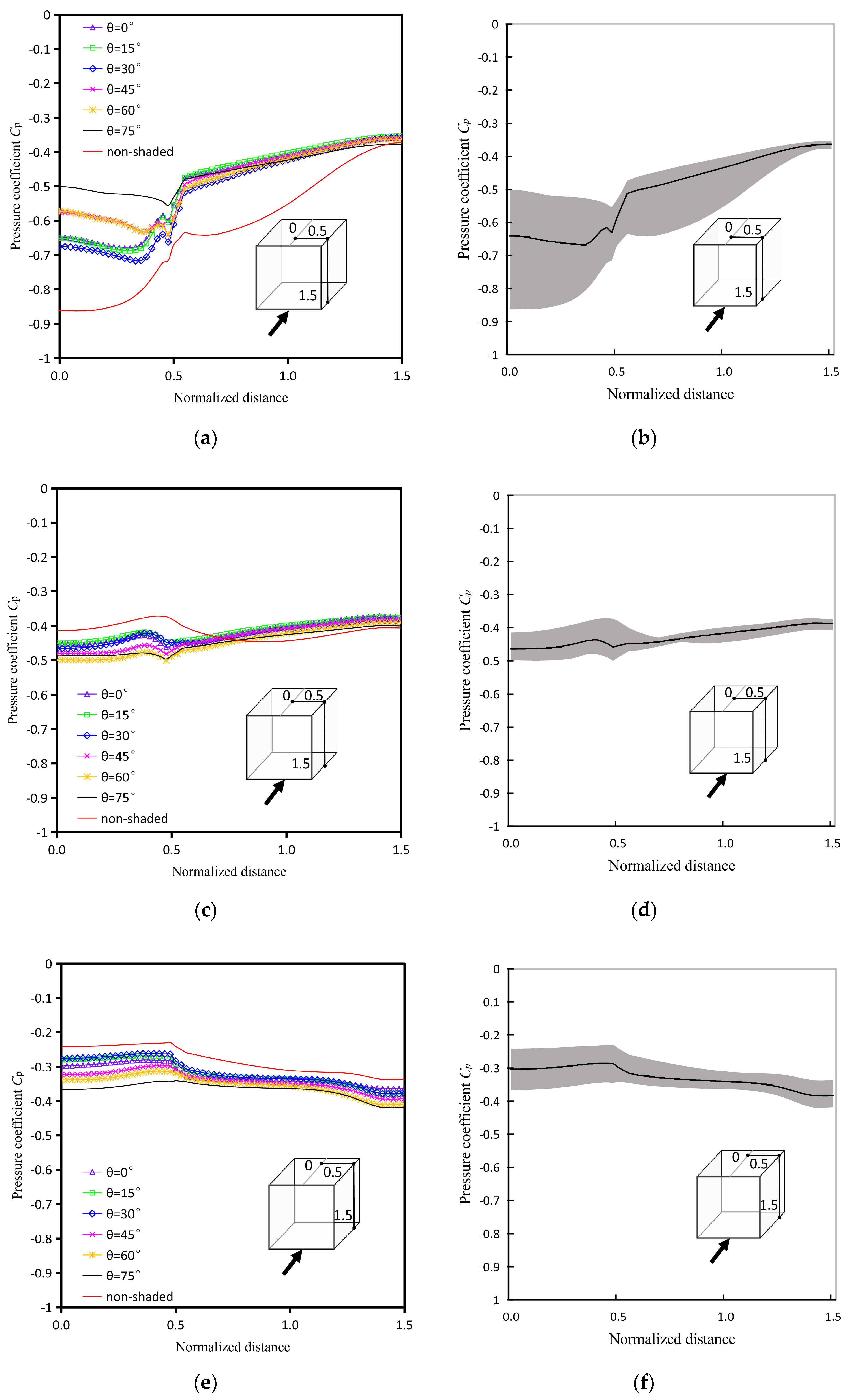
  • In general, the fluctuations of Cp on the windward and roof surfaces are mostly stronger than those on the lateral and leeward surfaces along the measurement lines. These results indicate that when the ventilation openings located on the roof and windward facade with louvers, the ventilation routes can lead to larger fluctuations of ventilation rate. In building design, it is important to diagnose the risks of inadequate ventilation for shaded buildings, especially those with roof ventilation systems.
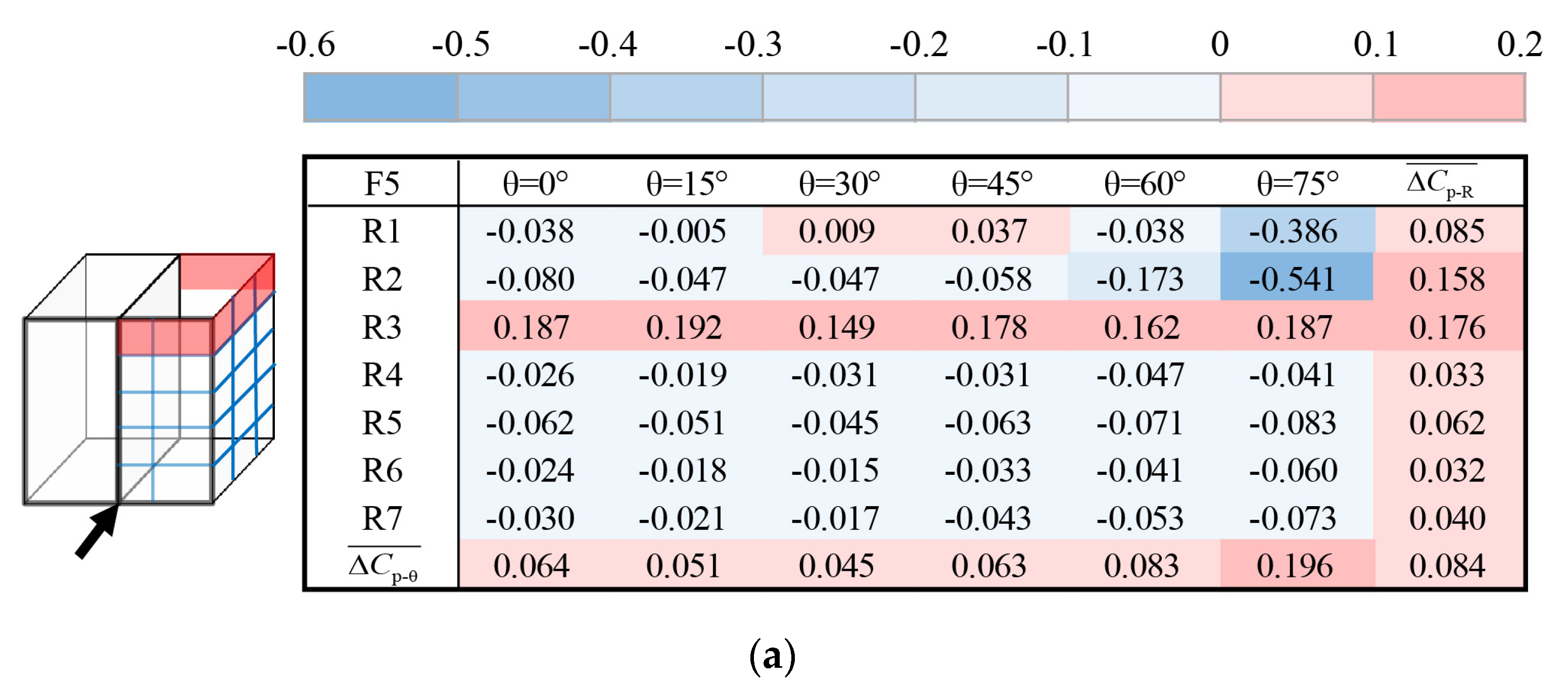
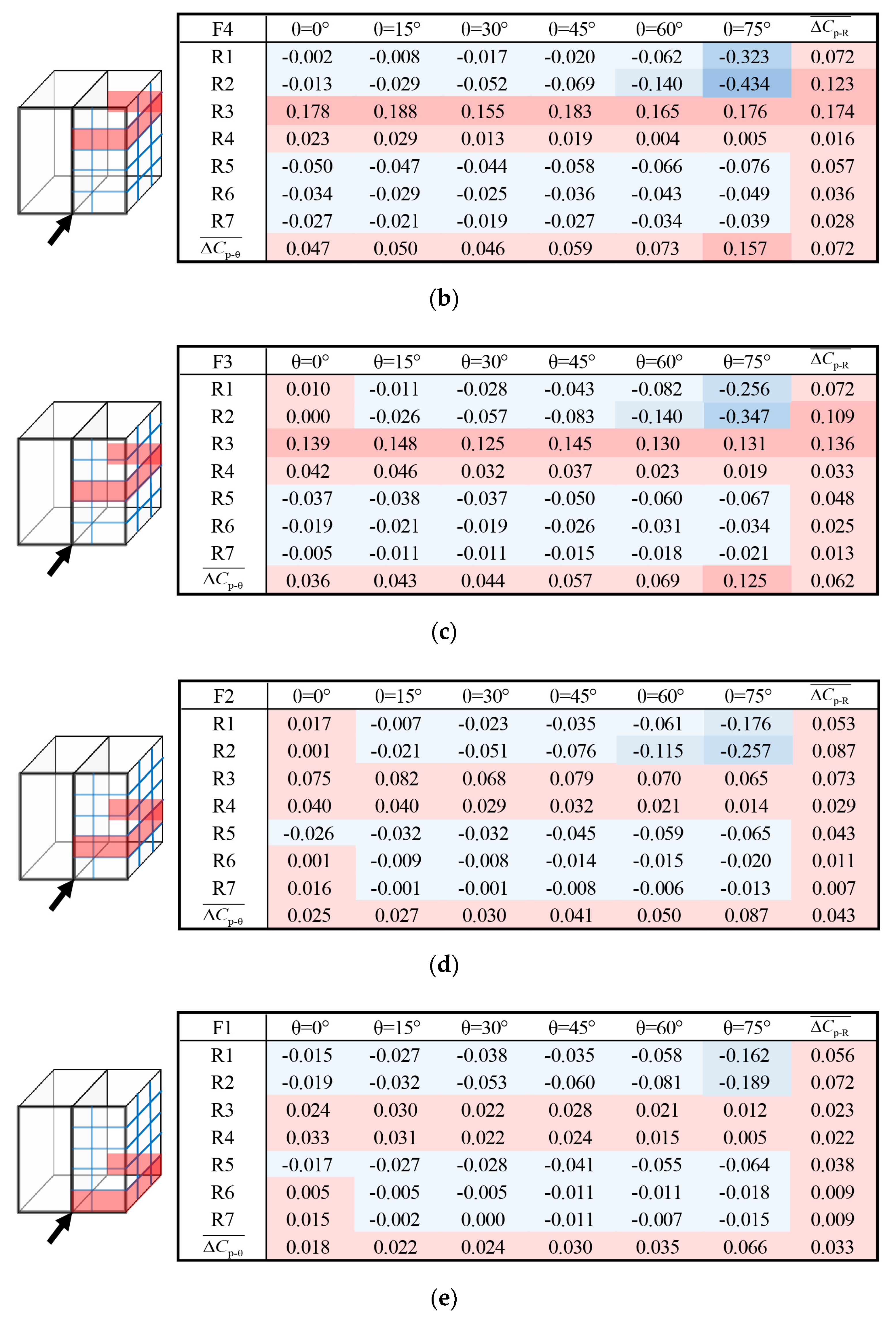
  • The stagnation zone of the windward surface has the highest average wind pressure coefficient C p ¯ . For most floors and rows, C p ¯ decreases with a higher rotation angle θ. And C p ¯ has the greatest reduction for all floors when θ turns from 60° to 75°. These results indicate that ventilation openings on the stagnation zone contribute to higher ventilation rate for the windward facade with louvers. When the rotation angle is taken for more than 60°, it is essential to avoid bad indoor wind environment for rooms with ventilation openings located on the shaded facade.
Overall, several parameters of wind pressure coefficient distribution were investigated in this study to gain a greater understanding of fluctuations in wind characteristics caused by the presence of external shading louvers. These kinds of data provide a wider perspective for building engineers and designers to understand the wind-induced fields around shaded buildings and improve the indoor environment in buildings with external shading louvers.

Author Contributions

Conceptualization, J.Z., Q.T. and L.L.; methodology, J.Z. and Q.T.; software, J.Z.; validation, J.Z. and Q.T.; formal analysis, J.Z., Q.T. and L.L.; investigation, J.Z.; writing—original draft preparation, J.Z.; writing—review and editing, J.Z., Q.T. and L.L.; visualization, J.Z. All authors have read and agreed to the published version of the manuscript.

Funding

This research was funded by the National Natural Science Foundation of China, Grant No. 51508225; Natural Science Foundation of Fujian Province, Grant No. 2018J01486; Foundation of Education Department of Fujian Province, Grant No. B16162, No. B18221; Jimei University Doctoral Research Initiation Fund, Grant No. ZQ2018006.

Conflicts of Interest

The authors declare no conflict of interest.

Nomenclature

Aopening area
ARarea of the outside surface of a room
Blouver width
Cddischarge coefficient
Cpwind pressure coefficient
Cp-maxmaximum wind pressure coefficient
Cp-minminimum wind pressure coefficient
Cμempirical constant
F1, F2, F3, F4, F5labels for different floors
h0reference height (m)
ishaded condition
Iturbulent intensity
jbuilding row
kturbulent kinetic energy (m2/s2)
Pstatic pressure
Piindoor pressure
Prefstatic pressure at the reference point
Qwind-induced airflow rate (m3/s)
Rrange of wind pressure coefficient
R1, R2, R3, R4, R5, R6, R7labels for different rows
Uwind velocity (m/s)
U(z)wind velocity at the height z (m/s)
Unnormalized velocity
Urefreference velocity
Wdistance between louvers and the windward facade
x, y, zcoordinates
y+dimensionless wall distance
αcoefficient for power-law profile of wind velocity
εturbulence dissipation rate (m2/s3)
θrotation angle of external shading louvers (°)
ρair density
SRarea of a grid on the outside surface
C p ¯ average wind pressure coefficient
Δ C p ¯ difference of average wind pressure coefficient between a shaded condition and the non-shaded condition
Δ C p - R ¯ average difference of wind pressure coefficient for all shaded conditions compared with the non-shaded condition in a special row
Δ C p - θ ¯ average difference of wind pressure coefficient between a specific shaded condition and the non-shaded condition in a whole row
C p - n ¯ average wind pressure coefficient in the non-shaded condition
C p - R - j ¯ average wind pressure coefficient in a specific row j
C p - θ - i ¯ average value of wind pressure coefficient for the shaded condition i with a specific rotation angle θ

References

  1. Eom, J.; Clarke, L.E.; Kim, S.H.; Kyle, G.P.; Patel, P.L. China’s Building Energy Use: A Long-Term Perspective Based on a Detailed Assessment; Pacific Northwest National Lab.: Richland, WA, USA, 2012. [Google Scholar]
  2. Kirimtat, A.; Koyunbaba, B.K.; Chatzikonstantinou, I.; Sariyildiz, S. Review of simulation modeling for shading devices in buildings. Renew. Sustain. Energy Rev. 2016, 53, 23–49. [Google Scholar] [CrossRef]
  3. Littlefair, P.; Ortiz, J.; Bhaumik, C.D. A simulation of solar shading control on UK office energy use. Build. Res. Inf. 2010, 38, 638–646. [Google Scholar] [CrossRef]
  4. Liu, M.; Wittchen, K.B.; Heiselberg, P.K. Control strategies for intelligent glazed façade and their influence on energy and comfort performance of office buildings in Denmark. Appl. Energy 2015, 145, 43–51. [Google Scholar] [CrossRef]
  5. Stazi, F.; Marinelli, S.; Di Perna, C.; Munafò, P. Comparison on solar shadings: Monitoring of the thermo-physical behaviour, assessment of the energy saving, thermal comfort, natural lighting and environmental impact. Sol. Energy 2014, 105, 512–528. [Google Scholar] [CrossRef]
  6. Tao, Q.H.; Li, Z.; Zheng, J.; Chen, X. Model of solar diffuse radiation transmission through circular perforated louvers and experimental verification. Energy Build. 2017, 142, 49–55. [Google Scholar] [CrossRef]
  7. Tao, Q.H.; Li, Z.; Zheng, J.; Jiang, F. A mathematical model for calculating total transmission of solar radiation through shuttle louvers and experimental verification. Energy Build. 2018, 172, 159–169. [Google Scholar] [CrossRef]
  8. Konstantzos, I.; Tzempelikos, A.; Chan, Y.C. Experimental and simulation analysis of daylight glare probability in offices with dynamic window shades. Build Environ. 2015, 87, 244–254. [Google Scholar] [CrossRef]
  9. Tablada, A.; Carmeliet, J.; Baelmans, M.; Saelens, D. Exterior Louvers as a Passive Cooling Strategy in a Residential Building: Computational fluid dynamics and building energy simulation modelling. In Proceedings of the 26th Conference on Passive and Low Energy Architecture, Quebec City, QC, Canada, 22–24 June 2009. [Google Scholar]
  10. Chandrashekaran, D. Air Flow through Louvered Openings: Effect of Louver Slats on Air Movement inside a Space. Master Thesis, University of Southern California, Los Angeles, CA, USA, 2010. [Google Scholar]
  11. Sun, N.; Cui, Y.; Jiang, Y. Lighting and Ventilation-based Building Sun-Shading Design and Simulation Case in Cold Regions. Energy Procedia 2018, 152, 462–469. [Google Scholar] [CrossRef]
  12. Kosutova, K.; van Hooff, T.; Vanderwel, C.; Blocken, B.; Hensen, J. Cross-ventilation in a generic isolated building equipped with louvers: Wind-tunnel experiments and CFD simulations. Build Environ. 2019, 154, 263–280. [Google Scholar] [CrossRef]
  13. Karava, P.; Stathopoulos, T.; Athienitis, A.K. Wind driven flow through openings–a review of discharge coefficients. Int. J. Vent. 2004, 3, 255–266. [Google Scholar] [CrossRef]
  14. Larsen, T.S. Natural Ventilation Driven by Wind and Temperature Difference. Ph.D. Thesis, Aalborg University, Aalborg, Denmark, 2006. [Google Scholar]
  15. Etheridge, D. Natural ventilation of buildings theory measurement and design. Int. J. Vent. 2011, 10, 405–406. [Google Scholar] [CrossRef]
  16. American Society of Heating, Refrigerating and Air-Conditioning Engineers Inc. ASHRAE Handbook Fundamentals; American Society of Heating, Refrigerating and Air-Conditioning Engineers Inc.: Atlanta, GA, USA, 2013. [Google Scholar]
  17. Montazeri, H.; Blocken, B. CFD simulation of wind-induced pressure coefficients on buildings with and without balconies: Validation and sensitivity analysis. Build Environ. 2013, 60, 137–149. [Google Scholar] [CrossRef]
  18. Gullbrekken, L.; Uvsløkk, S.; Kvande, T.; Pettersson, K.; Time, B. Wind pressure coefficients for roof ventilation purposes. J. Wind. Eng. Ind. Aerod. 2018, 175, 144–152. [Google Scholar] [CrossRef]
  19. Hong, X.; He, W.; Hu, Z.; Wang, C.; Ji, J. Three-dimensional simulation on the thermal performance of a novel Trombe wall with venetian blind structure. Energy Build. 2015, 89, 32–38. [Google Scholar] [CrossRef]
  20. Zeng, Z.; Li, X.; Li, C.; Zhu, Y. Modeling ventilation in naturally ventilated double-skin façade with a venetian blind. Build Environ. 2012, 57, 1–6. [Google Scholar] [CrossRef]
  21. Richards, P.J.; Hoxey, R.P.; Short, L.J. Wind pressures on a 6m cube. J. Wind. Eng. Ind. Aerod. 2001, 89, 1553–1564. [Google Scholar] [CrossRef]
  22. Richards, P.J.; Hoxey, R.P. Pressures on a cubic building—Part 1: Full-scale results. J. Wind. Eng. Ind. Aerod. 2012, 102, 72–86. [Google Scholar] [CrossRef]
  23. Richardson, G.M.; Surry, D. The Silsoe structures building: Comparison between full-scale and wind-tunnel data. J. Wind. Eng. Ind. Aerod. 1994, 51, 157–176. [Google Scholar] [CrossRef]
  24. Guan, Y.; Li, A.; Zhang, Y.; Jiang, C.; Wang, Q. Experimental and numerical investigation on the distribution characteristics of wind pressure coefficient of airflow around enclosed and open-window buildings. Build. Simul. 2016, 9, 551–568. [Google Scholar] [CrossRef]
  25. Yang, L.; Gurley, K.R.; Prevatt, D.O. Probabilistic modeling of wind pressure on low-rise buildings. J. Wind. Eng. Ind. Aerod. 2013, 114, 18–26. [Google Scholar] [CrossRef]
  26. Gomes, M.G.; Rodrigues, A.M.; Mendes, P. Experimental and numerical study of wind pressures on irregular-plan shapes. J. Wind. Eng. Ind. Aerod. 2005, 93, 741–756. [Google Scholar] [CrossRef]
  27. Holmes, J.D.; Carpenter, P. The effect of Jensen Number variations on the wind loads on a low-rise building. J. Wind. Eng. Ind. Aerod. 1990, 36, 1279–1288. [Google Scholar] [CrossRef]
  28. Grosso, M. Wind pressure distribution around buildings: A parametrical model. Energy Build. 1992, 18, 101–131. [Google Scholar] [CrossRef]
  29. Lou, W.; Huang, M.; Zhang, M.; Lin, N. Experimental and zonal modeling for wind pressures on double-skin facades of a tall building. Energy Build. 2012, 54, 179–191. [Google Scholar] [CrossRef]
  30. Muehleisen, R.T.; Patrizi, S. A new parametric equation for the wind pressure coefficient for low-rise buildings. Energy Build. 2013, 57, 245–249. [Google Scholar] [CrossRef]
  31. Shen, X.; Zhang, G.; Bjerg, B. Comparison of different methods for estimating ventilation rates through wind driven ventilated buildings. Energy Build. 2012, 54, 297–306. [Google Scholar] [CrossRef]
  32. Liu, J.; Niu, J. CFD simulation of the wind environment around an isolated high-rise building: An evaluation of SRANS, LES and DES models. Build Environ. 2016, 96, 91–106. [Google Scholar] [CrossRef]
  33. Cóstola, D.; Blocken, B.; Hensen, J.L.M. Overview of pressure coefficient data in building energy simulation and airflow network programs. Build Environ. 2009, 44, 2027–2036. [Google Scholar] [CrossRef] [Green Version]
  34. Ramponi, R.; Blocken, B. CFD simulation of cross-ventilation for a generic isolated building: Impact of computational parameters. Build Environ. 2012, 53, 34–48. [Google Scholar] [CrossRef]
  35. Kato, S.; Murakami, S.; Mochida, A.; Akabayashi, S.I.; Tominaga, Y. Velocity-pressure field of cross ventilation with open windows analyzed by wind tunnel and numerical simulation. J. Wind. Eng. Ind. Aerod. 1992, 41, 2575–2586. [Google Scholar] [CrossRef]
  36. Karava, P.; Stathopoulos, T.; Athienitis, A.K. Wind-induced natural ventilation analysis. Sol. Energy 2007, 81, 20–30. [Google Scholar] [CrossRef]
  37. Liu, X.; Niu, J.; Kwok, K.C.S. Evaluation of RANS turbulence models for simulating wind-induced mean pressures and dispersions around a complex-shaped high-rise building. Build. Simul. 2013, 6, 151–164. [Google Scholar] [CrossRef]
  38. Ramponi, R.; Angelotti, A.; Blocken, B. Energy saving potential of night ventilation: Sensitivity to pressure coefficients for different European climates. Appl. Energy 2014, 123, 185–195. [Google Scholar] [CrossRef]
  39. Peng, X.; Yang, L.; Gavanski, E.; Gurley, K.; Prevatt, D. A comparison of methods to estimate peak wind loads on buildings. J. Wind. Eng. Ind. Aerod. 2014, 126, 11–23. [Google Scholar] [CrossRef]
  40. Kim, G.; Lim, H.S.; Lim, T.S.; Schaefer, L.; Kim, J.T. Comparative advantage of an exterior shading device in thermal performance for residential buildings. Energy Build. 2012, 46, 105–111. [Google Scholar] [CrossRef]
  41. Cóstola, D.; Blocken, B.; Ohba, M.; Hensen, J.L.M. Uncertainty in airflow rate calculations due to the use of surface-averaged pressure coefficients. Energy Build. 2010, 42, 881–888. [Google Scholar] [CrossRef] [Green Version]
  42. Mou, B.; He, B.J.; Zhao, D.X.; Chau, K.W. Numerical simulation of the effects of building dimensional variation on wind pressure distribution. Eng. Appl. Comp. Fluid. Mech. 2017, 11, 293–309. [Google Scholar] [CrossRef]
  43. Cóstola, D.; Blocken, B.; Hensen, J.L.M. Uncertainties due to the use of surface averaged wind pressure coefficients. In Proceedings of the 29th AIVC Conference, Kyoto, Japan, 14–16 October 2008. [Google Scholar]
  44. Jiang, F.; Li, Z.; Zhao, Q.; Tao, Q.; Yuan, Y.; Lu, S. Flow field around a surface-mounted cubic building with louver blinds. Build. Simul. 2019, 12, 141–151. [Google Scholar] [CrossRef]
  45. Zheng, J.; Tao, Q.; Li, L. Study of influence of shading louvers on wind characteristics around buildings under different wind directions. In Proceedings of the 4th Asia Conference of International Building Performance Simulation Association, Hong Kong, China, 3–5 December 2018. [Google Scholar]
  46. Franke, J. Recommendations of the COST action C14 on the use of CFD in predicting pedestrian wind environment. In Proceedings of the Fourth International Symposium on Computational Wind Engineering, Yokohama, Japan, 16–19 July 2006. [Google Scholar]
  47. Tominaga, Y.; Mochida, A.; Yoshie, R.; Kataoka, H.; Nozu, T.; Yoshikawa, M.; Shirasawa, T. AIJ guidelines for practical applications of CFD to pedestrian wind environment around buildings. J. Wind. Eng. Ind. Aerod. 2008, 96, 1749–1761. [Google Scholar] [CrossRef]
  48. Versteeg, H.K.; Malalasekera, W. An Introduction to Computational Fluid Dynamics: The Finite Volume Method; Pearson Education: London, UK, 2007. [Google Scholar]
  49. Toparlar, Y.; Blocken, B.; Maiheu, B.; van Heijst, G.J.F. A review on the CFD analysis of urban microclimate. Renew. Sustain. Energy Rev. 2017, 80, 1613–1640. [Google Scholar] [CrossRef]
  50. Meng, F.Q.; He, B.J.; Zhu, J.; Zhao, D.X.; Darko, A.; Zhao, Z.Q. Sensitivity analysis of wind pressure coefficients on CAARC standard tall buildings in CFD simulations. J. Build. Eng. 2018, 16, 146–158. [Google Scholar] [CrossRef]
  51. ANSYS, Inc. ANSYS Fluent Theory Guide; ANSYS, Inc.: Canonsburg, PA, USA, 2013. [Google Scholar]
  52. Roache, P.J. Perspective: A method for uniform reporting of grid refinement studies. J. Fluid. Eng. 1994, 116, 405–413. [Google Scholar] [CrossRef]
  53. Roache, P.J. Quantification of uncertainty in computational fluid dynamics. Annu. Rev. Fluid. Mech. 1997, 29, 123–160. [Google Scholar] [CrossRef] [Green Version]
  54. Vinchurkar, S.; Longest, P.W. Evaluation of hexahedral, prismatic and hybrid mesh styles for simulating respiratory aerosol dynamics. Comput. Fluids 2008, 37, 317–331. [Google Scholar] [CrossRef]
  55. Blocken, B. Computational fluid dynamics for urban physics: Importance, scales, possibilities, limitations and ten tips and tricks towards accurate and reliable simulations. Build Environ. 2015, 91, 219–245. [Google Scholar] [CrossRef] [Green Version]
  56. Mochida, A.; Lun, I.Y.F. Prediction of wind environment and thermal comfort at pedestrian level in urban area. J. Wind. Eng. Ind. Aerod. 2008, 96, 1498–1527. [Google Scholar] [CrossRef]
  57. Shirzadi, M.; Mirzaei, P.A.; Naghashzadegan, M. Improvement of k-epsilon turbulence model for CFD simulation of atmospheric boundary layer around a high-rise building using stochastic optimization and Monte Carlo Sampling technique. J. Wind. Eng. Ind. Aerod. 2017, 171, 366–379. [Google Scholar] [CrossRef]
Figure 1. Control system of shading louvers.
Applsci 10 01128 g001
Figure 2. Geometry model of the cube building with shading louvers.
Applsci 10 01128 g002
Figure 3. Measurement lines on the central plane of the studied building for (a) velocity U; and (b) wind pressure coefficient Cp.
Applsci 10 01128 g003
Figure 4. Wind characteristics of approaching flow for computational fluid dynamics CFD simulation: (a) velocity U; and (b) turbulent intensity I distributions.
Applsci 10 01128 g004
Figure 5. Flowchart for investigating airflow fields of the shaded building.
Applsci 10 01128 g005
Figure 6. Dimensions of the computational domain for CFD simulation.
Applsci 10 01128 g006
Figure 7. Grid resolution for the reference case: (a) global grid resolution; (b) grid resolution around the building and louvers.
Applsci 10 01128 g007
Figure 8. Comparison of normalized velocity U/Uref distribution around the building on the measurement line: (a) 2.5h0, (b) 1.5h0, (c) 0.5h0 and (d) −0.5h0.
Applsci 10 01128 g008
Figure 9. Comparison of wind pressure coefficient Cp distribution.
Applsci 10 01128 g009
Figure 10. Airflow pattern and wind pressure distribution. (a) Airflow towards the central rows; (b) Airflow towards the side rows.
Applsci 10 01128 g010
Figure 11. Arrangement of rooms and measurement lines. (a) Locations of seven rows and five floors, (b) W-R-L lines along windward, roof and leeward surfaces; (c) W-S-L lines along windward, lateral and leeward surfaces; and (d) R-S lines along roof and lateral surfaces.
Applsci 10 01128 g011
Figure 12. Local range R, local and average value of wind pressure coefficient Cp for different shaded conditions on the central lines of different rows along the windward, roof and leeward surfaces. (a) Local value along R1 and R7; (b) Local range R and average value along R1 and R7; (c) Local value along R2 and R6; (d) Local range R and average value along R2 and R6.
Applsci 10 01128 g012
Figure 13. Local range R, local and average value of wind pressure coefficient Cp for different shaded conditions on the central lines of different floors along the windward, lateral and leeward surfaces. (a) Local value along F1; (b) Local range R and average value along F1; (c) Local value along F2; (d) Local range R and average value along F2; (e) Local value along F3; (f) Local range R and average value along F3; (g) Local value along F4; (h) Local range R and average value along F4; (i) Local value along F5; (j) Local range R and average value along F5.
Applsci 10 01128 g013aApplsci 10 01128 g013bApplsci 10 01128 g013c
Figure 14. Local range R, local and average value of wind pressure coefficient Cp for different shaded conditions on the central lines of different rows along the roof and lateral surfaces. (a) Local value along R3; (b) Local range R and average value along R3; (c) Local value along R4; (d) Local range R and average value along R4; (e) Local value along R5; (f) Local range R and average value along R5.
Applsci 10 01128 g014
Figure 15. Average wind pressure coefficient C p ¯ on outside surfaces of rooms under different shaded conditions for (a) R1; (b) R2; (c) R3; (d) R4; (e) R5; (f) R6; (g) R7.
Applsci 10 01128 g015aApplsci 10 01128 g015b
Figure 16. Difference Δ C p ¯ of average wind pressure coefficient C p ¯ between different shaded conditions and the non-shaded condition for (a) F5; (b) F4; (c) F3; (d) F2; (e) F1.
Applsci 10 01128 g016aApplsci 10 01128 g016b
Table 1. Comparison of average value of normalized velocity U/Uref and wind pressure coefficient Cp on measurement lines.
Value TypeU/UrefCp
−0.5h00.5h01.5h02.5h0WindwardRoofLeeward
Average value (reference case)1.210.941.030.720.62−0.45−0.19
Average value (Jiang et al.)1.220.971.050.740.6−0.45−0.18
Absolute deviation0.080.050.040.10.030.090.02

