Uncertainty Analysis of 3D Line Reconstruction in a New Minimal Spatial Line Representation

Abstract

Line segments are common in urban scenes and contain rich structural information. However, different from point-based reconstruction, reconstructed 3D lines may have large displacement from the ground truth in spite of a very small sum of reprojection error. In this work, we present a method to analyze the uncertainty of line reconstruction and provide a quantitative evaluation of accuracy. A new minimal four-vector line representation based on Plücker line is introduced, which is tailed for uncertainty analysis of line reconstruction. Each component of the compact representation has a certain physical meaning about the 3D line’s orientation or position. The reliability of the reconstructed lines can be measured by the confidence interval of each component in the proposed representation. Based on the uncertainty analysis of two-view line triangulation, the uncertainty of multi-view line reconstruction is also derived. Combining the proposed uncertainty analysis with reprojection error, a more reliable 3D line map can be obtained. Experiments on simulation data, synthetic and real-world image sequences validate the feasibility of the proposed method.

1. Introduction

Recovering 3D structure from 2D images captured from different views is an important and basic task of computer vision. Benefited from point feature detectors and descriptors, the point-based reconstruction received major attention. However, line segments are common in urban scenes and provide more intuitive structural information. Though more complicated than point reconstruction, line construction is meaningful for urban and poorly-textured scenes. Recently, line segments are widely applied to structure from motion [1,2,3,4], SLAM systems [5,6,7,8,9,10], visual odometry algorithms [11,12], mapping [13,14,15,16] and modelling [17]. Compared with point reconstruction, line reconstruction suffers from much more severe degeneracy [18]. Lines coplanar with two camera centers cannot be determined by triangulation these two observations. Lines that are close to the epipolar plane can be poorly localized even with a large baseline and a small reprojection error. In 3D reconstruction, reprojection error has always been a golden rule to evaluate the accuracy of reconstructed points of lines. In general cases, the setting threshold on reprojection can reject poorly reconstructed lines from wrong matches. However, small reprojection error does not guarantee a well-reconstructed line in nearly-degenerate cases and fails to provide a numerical evaluation of direction or location accuracy of the line in 3D. When cameras are mounted on a car and move along the road, many lines on the buildings along the road are approximately coplanar with camera motion. It is necessary to analyze the uncertainty of the reconstructed lines to distinguish those lines that are badly reconstructed with a high probability. In this work, we focus on uncertainty analysis of 3D line reconstruction and intend to provide a numerical evaluation of the reconstruction accuracy, with which a more reliable line map can be obtained.

1.1. Related Work

Degeneracy and map culling in 3D line reconstruction. Spatial lines can be reconstructed from observations with known poses and further can be used to determine the poses of new cameras. Different from triangulation for points, line segment correspondences between two views do not have any geometry constraints. The line can be solved uniquely by intersecting two projection planes. We can’t measure the accuracy by reprojection error as in two-view triangulation for 3D points. Using more observations and minimizing the sum of reprojection errors in all observed images is a convention of estimating a spatial line. To make things worse, degeneracy for line triangulation is far more severe than for point triangulation [18]. In degenerate cases, lines will be reconstructed with large uncertainties. To deal specifically with the degeneracy, the detected line segments that are nearly-aligned (≤10°) with the epipolar line were labeled as degenerated cases in [13] and [19]. Ref. [17] avoided degeneracy by measuring the distance between the reconstructed 3D line and the camera baseline. Ref. [20,21] detected degenerate cases by measuring the angular span of all projection planes’ normal vectors. However, these methods specify degeneracy by setting thresholds on some parameters with personal experience.

Small reprojection errors and large baselines do not guarantee a well-reconstructed line. Most of the existing line reconstruction work does not consider the degeneracy specifically. To get a reliable line map, lines seen from less than three viewpoints or in less than 25% of the frames from which they were expected to be seen were discarded in [6]. In Hofer’s series of work on 3D line reconstruction [14,16], clustering approaches [22,23] were applied to generate the final line-based 3D model. Ref. [15] proposed to eliminate outliers by line grouping, a representative line was estimated for each group and these lines that do not form a group with at least one other line were discarded. In the group-based methods, some lines that are no outliers but different 3D lines are merged into one line. Though effective to some extent, these methods generally need sufficient observations to ensure a good line thus not suitable for limited views. Many poorly localized lines will present in the final line map if we simply set a threshold on the reprojection error. Subsequent motion estimation and mesh generation will suffer from these badly reconstructed lines.

Uncertainty of 3D reconstruction. Uncertainty is a common criterion used to measure the reliability of estimations. The estimation and propagation of uncertainty have been well studied mathematically [18,24]. The uncertainties of reconstruction parameters can be obtained by propagating the uncertainties of input parameters, i.e., detected features in images. Depth uncertainty of point reconstruction has been well-studied [25,26,27,28,29]. Recently, [30] proposed an efficient algorithm for uncertainty propagation which works with large scale 3D reconstruction. In comparison, the research on the uncertainty of line reconstruction is much less. Ref. [31] analyzed the stereo line reconstruction and demonstrated that a line can be more accurately reconstructed as an intersection of two planes than reconstructing pair of endpoints. To be more general, [32] presented a performance analysis of reconstructing a 3D line from two arbitrary perspective views. A spatial line was represented by three direction cosines and a point on the line. Inverse perspective equations were derived to describe 3D line error. Simulation experiments were conducted to illustrate the effect of multiple factors on errors in line reconstruction. Ref. [33] analyzed error generation and propagation in a multilayer feature graph including line segments, and used them as observation error models in the extended Kalman filter. Uncertainty of 2D line segment extraction in images and 3D line segment extraction by RGB-D sensors are investigated. A 3D line reconstruction using uncertain projective geometry was proposed in [34]. The results need to be improved because only geometry information is used. Although a series of qualitative measures have been proposed to achieve better reconstruction, quantitative measurements of line reconstruction accuracy are still missing.

Representations of 3D lines. The widely adopted representation methods of spatial lines can be divided into two types according to the number of parameters: the linear over-parametrization and the nonlinear minimal four-parameter [2]. The linear over-parametrization representations are suitable for expressing transformation and projection, while the nonlinear minimal four-parameter representations are more favorable for nonlinear optimization. For the first type, a 3D line can be represented by two endpoints [5,6,7,8], the closest point and direction [35], pair of points or pair of planes [18], or Plücker lines [12,19,36,37,38]. For the nonlinear minimal four-parameter representations, a 3D line was represented by the intersection of two certain planes in [39], then lines parallel to both planes can not be represented. The orthonormal representation of spatial lines was proposed in [1]. There is no internal gauge freedom in the orthonormal representation thus well-suited for optimization. Ref. [10] utilized the orthonormal representation to deal with parameter redundancy in the backend of visual SLAM. In [2], the Plücker lines were transformed into four-vector by Cayley transform [40] to automatically guarantee that the parameters of lines satisfied the Plücker constraints. In both methods, spatial lines are represented in other spaces or by relation with other spaces, the orientation and location are expressed indirectly. Ref. [41] proposed to use two angles and a 2D coordinates to represent a 3D line. Two angles were used to indicate the direction of the line in 3D space. The location was indirectly indicated by a 2D coordinates on the plane that passes through the origin and is perpendicular to the direction. For the special case in [21], a 3D line on the reference frame is parameterized by an angle to specify the direction and a variable $\lambda$ to specify the location on the projection plane.

Redundant spatial line representation methods are not suitable for uncertainty analysis. The redundancy in the representation leads to singular covariance matrices and thus there is no proper probability density function (PDF). Besides, a 3D line has four degrees of freedom, hence it is not easy to visualize the uncertainty by the confidence region. As we know, the confidence region of a one-dimensional variable is a one-dimensional interval, the confidence region of a two-dimensional variable is a two-dimensional ellipse, and the confidence region of a three-dimensional variable is a three-dimensional ellipsoid. Variables with dimensions greater than four are more difficult to visually represent their confidence regions. In order to intuitively visualize the uncertainty and easily evaluate the reliability of the reconstruction line, we expect a minimal spatial line representation that meets two conditions: uses non-redundant form to represent the direction and position of the line in three-space; each component corresponds to a motion type of the line in three-space, then the uncertainty can be interpreted as confidence interval lengths of all components.

1.2. Contributions

In this paper, an uncertainty analysis method for line reconstruction is proposed to provide a quantitative evaluation of reconstruction accuracy. The proposed uncertainty analysis is able to distinguish poorly reconstructed lines resulting from line triangulation under insufficient effective ego-motion. Based on the Plücker line representation, a minimal four-vector line representation is proposed. In the proposed representation, each component has a clear physical meaning that describes orientation or position of the line in 3D. The uncertainty of a spatial line can be easily visualized by representing the direction and position with two parameters, respectively. The reliability of an estimated line is interpreted as the confidence interval of every component. Based on the uncertainty analysis of two-view triangulation, the uncertainty analysis can be extended to multi-view line reconstruction. The lines that have a large probability of being inaccurately reconstructed can be rejected by uncertainty rejection. The feasibility of the proposed uncertainty analysis method is validated by experiments on simulation data. The application in map-culling of the proposed uncertainty analysis is tested on synthetic and real-world dataset, experimental results show that a more reliable 3D line map can be obtained by incorporating the reprojection error and the proposed uncertainty analysis in outlier rejection.

2. The Proposed Method

In this section, a detailed description of the uncertainty analysis of 3D line reconstruction is presented. It is a wise choice to use different representations according to stages of line reconstruction. In this work, the Plücker line representation is applied in projection and triangulation. A 3D line is computed in Plücker coordinates and then converted into the proposed line representation for uncertainty estimation and analysis. Spatial line representation and triangulation in Plücker coordinates are introduced in Section 2.1. A minimal spatial line representation is introduced in Section 2.2. The relationship between the proposed line representation and the Plücker line representation is introduced in Section 2.3. The uncertainty estimation and visualization of two-view line reconstruction are described in Section 2.4. Based on the two-view triangulation, Section 2.5 introduces the uncertainty update of multi-view 3D line reconstruction.

2.1. Notations on 3D Line Representation and Triangulation in Plücker Coordinates

In this paper, we use the derivation of a Plücker line representation based on two given 3D points ${\mathbf{X}}_0$ and ${\mathbf{Y}}_0$ described in [42]:

$$\mathbf{L}({\mathbf{X}}_0,{\mathbf{Y}}_0)=\left(\frac{{\mathbf{Y}}_0-{\mathbf{X}}_0}{{\mathbf{X}}_0\times {\mathbf{Y}}_0}\right)=\left(\frac{{\mathbf{L}}_h}{{\mathbf{L}}_o}\right).$$

(1)

The first part ${\mathbf{L}}_h$ is homogeneous and indicates the direction of the line. The second part ${\mathbf{L}}_o$ is the normal of the plane defined by ${\mathbf{X}}_0$, ${\mathbf{Y}}_0$ and the origin, we can conclude that:

$${\mathbf{L}}_h^T{\mathbf{L}}_o={\mathbf{L}}_o^T{\mathbf{L}}_h=0.$$

(2)

A Plücker line is represented by two three-vectors: $\mathbf{L}=(\mathbf{m};\mathbf{d})$, while $\mathbf{d}$ denotes the direction and $\mathbf{m}$ denotes the momentum, corresponding to ${\mathbf{L}}_h$ and ${\mathbf{L}}_o$, respectively.

As derived in [19], the projection constraint equation of lines in Plücker coordinates is:

$$\left(\begin{array}{cc}{\left[{\mathbf{n}}_c^i\right]}_{\times }{\mathbf{R}}_{wc}^i& -{\left({\mathbf{n}}_c^i\right)}^{\mathrm{T}}{\mathbf{t}}_{wc}^i{\mathbf{R}}_{wc}^i\end{array}\right)\left(\begin{array}{c}\mathbf{m}\\ \mathbf{d}\end{array}\right)={\mathbf{0}}_{3\times 1},$$

(3)

where ${[·]}_{\times }$ denotes the skew-symmetric matrix of a three-dimensional vector, ${\mathbf{n}}_c^i$ denotes the normal vectors of projection plane in the i-th camera coordinate system, ${\mathbf{R}}_{wc}^i$ and ${\mathbf{t}}_{wc}^i$ denote the rotation and translation from the i-th camera coordinate system to the world coordinate system, respectively.

2.1.1. Two-View Line Triangulation

As illustrated in Figure 1, a 3D line $\mathbf{L}=(\mathbf{m};\mathbf{d})$ is projected to two cameras. ${\mathbf{O}}_w-XYZ$ denotes the world coordinate system. ${\mathbf{C}}_1$ and ${\mathbf{C}}_2$ are camera centers. Let ${\mathbf{R}}_{wc}^1$ and ${\mathbf{t}}_{wc}^1$ be the rotation and translation from camera 1 to the world coordinate system, ${\mathbf{R}}_{wc}^2$ and ${\mathbf{t}}_{wc}^2$ be the rotation and translation from camera 2 to the world coordinate system. ${\mathbf{p}}_s^1$, ${\mathbf{p}}_e^1$, ${\mathbf{p}}_s^2$ and ${\mathbf{p}}_e^2$ are the normalized homogeneous endpoints of the detected line segments in two images, respectively. ${\mathbf{n}}_c^1$ and ${\mathbf{n}}_c^2$ are the normal vectors of projection plane in respective camera coordinate system: ${\mathbf{n}}_c^1={\mathbf{p}}_s^1\times {\mathbf{p}}_e^1$, ${\mathbf{n}}_c^2={\mathbf{p}}_s^2\times {\mathbf{p}}_e^2$.

When $\mathbf{L}$ is projected to camera i, we can derive the constraint between $\mathbf{m}$ and $\mathbf{d}$:

$${\mathbf{S}}_i\mathbf{m}={\left({\mathbf{n}}_c^i\right)}^{\mathrm{T}}{\mathbf{t}}_{wc}^i\mathbf{d},$$

(4)

where ${\mathbf{S}}_i={\left({\mathbf{R}}_{wc}^i\right)}^{\mathrm{T}}{\left[{\mathbf{n}}_c^i\right]}_{\times }{\mathbf{R}}_{wc}^i$ is a skew-symmetry matrix defined by the pose of camera i. ${\mathbf{m}}^{\mathrm{T}}\mathbf{d}={\mathbf{m}}^{\mathrm{T}}{\mathbf{S}}_i\mathbf{m}/\left({\left({\mathbf{n}}_c^i\right)}^{\mathrm{T}}{\mathbf{t}}_{wc}^i\right)=0$, which satisfies the Plücker constraint. Given two different observations from ${\mathbf{C}}_1$ and ${\mathbf{C}}_2$(the line passing ${\mathbf{C}}_1$ and ${\mathbf{C}}_1$ should not be parallel to the direction of motion), we can solve the Plücker line by:

$$\begin{array}{cc}\hfill \mathbf{d}& =\frac{\left({\mathbf{R}}_{wc}^1{\mathbf{n}}_c^1\right)\times \left({\mathbf{R}}_{wc}^2{\mathbf{n}}_c^2\right)}{\left|\left({\mathbf{R}}_{wc}^1{\mathbf{n}}_c^1\right)\times \left({\mathbf{R}}_{wc}^2{\mathbf{n}}_c^2\right)\right|}\hfill \\ \hfill \mathbf{m}& ={\left({\mathbf{A}}^{\mathrm{T}}\mathbf{A}\right)}^{-1}{\mathbf{A}}^{\mathrm{T}}\mathbf{b}\hfill \end{array},$$

(5)

where:

$$\mathbf{A}={\left(\begin{array}{c}{\mathbf{S}}_1\\ {\mathbf{S}}_2\end{array}\right)}_{6\times 3},\mathbf{b}={\left(\begin{array}{c}{\left({\mathbf{n}}_c^1\right)}^{\mathrm{T}}{\mathbf{t}}_{wc}^1\mathbf{d}\\ {\left({\mathbf{n}}_c^2\right)}^{\mathrm{T}}{\mathbf{t}}_{wc}^2\mathbf{d}\end{array}\right)}_{6\times 1}.$$

(6)

2.1.2. Multi-View Line Reconstruction in Plücker Coordinates

Multiple observation constraints can be simply stacked to solve a Plücker line by linear equations. Given n observations of the line with $\{{\mathbf{R}}_{wc}^i,{\mathbf{t}}_{wc}^i,{\mathbf{n}}_c^i\}$, $i\in \{1,2,\cdots ,n\}$, the constrain equations can be written as:

$$\left(\begin{array}{cc}{\left[{\mathbf{n}}_c^1\right]}_{\times }{\mathbf{R}}_{wc}^1& -{\left({\mathbf{n}}_c^1\right)}^{\mathrm{T}}{\mathbf{t}}_{wc}^1{\mathbf{R}}_{wc}^1\\ {\left[{\mathbf{n}}_c^2\right]}_{\times }{\mathbf{R}}_{wc}^2& -{\left({\mathbf{n}}_c^2\right)}^{\mathrm{T}}{\mathbf{t}}_{wc}^2{\mathbf{R}}_{wc}^2\\ ⋮& ⋮\\ {\left[{\mathbf{n}}_c^n\right]}_{\times }{\mathbf{R}}_{wc}^n& -{\left({\mathbf{n}}_c^n\right)}^{\mathrm{T}}{\mathbf{t}}_{wc}^n{\mathbf{R}}_{wc}^n\end{array}\right)\left(\begin{array}{c}\mathbf{m}\\ \mathbf{d}\end{array}\right)={\mathbf{0}}_{3n\times 1}.$$

(7)

The least-squares solution of the Plücker line $\mathbf{L}=(\mathbf{m};\mathbf{d})$ can be found by decomposing the left matrix using Singular Value Decomposition(SVD).

2.2. A New Minimal Spatial Line Representation Tailored for Uncertainty Analysis

We expect a spatial line representation method that satisfies the following characteristics: a minimal four-vector representation whose direction and position use two parameters respectively; each parameter corresponds to a clear physical meaning of the line in three-dimensional space, and it can be intuitively imagined how the spatial line moves as each parameter changes.

A three-dimensional unit direction vector can be mapped as a point on the unit sphere, which in turn can be represented by a spherical coordinate of two dimensions. In addition to direction, the distance from the origin to the line is also an important attribute of the line. By fixing the direction and the distance to the origin, we can get a set of spatial lines. This set of lines are all tangent of a 3D circle in space, as illustrated in Figure 2. By specifying a point ${\mathbf{P}}_c$ on the circle, a spatial line can be uniquely determined. The position of ${\mathbf{P}}_c$ on the circle can be represented by an angular interval with the length of 2$\pi$.

In this paper, we propose to represent a spatial line $\mathbf{L}$ by $(\theta ,\varphi ,m_l,\alpha )$. $\theta$ and $\varphi$ are used to describe the direction in the spherical coordinate system:

$$\mathbf{d}(\theta ,\varphi )={(sin\theta cos\varphi ,sin\theta sin\varphi ,cos\theta )}^{\mathrm{T}}.$$

(8)

Figure 3 illustrates how the line direction varies with $\theta$ and $\varphi$. $m_l$ denotes the distance between the line and the origin. As showed in Figure 2, a spatial line with fixed direction and distance to the origin can be determined only if the point ${\mathbf{P}}_c$ is specified. At the same time, ${\mathbf{P}}_c$ is the closest point from the origin to the line. To specify the position of ${\mathbf{P}}_c$, we define an artificial intermediate variable ${\mathbf{v}}_s$ which is perpendicular to the direction vector $\mathbf{d}$ and passes the origin. Then ${\mathbf{v}}_s$ is coplanar with the red circle in Figure 2. The rotation from ${\mathbf{v}}_s$ to ${\mathbf{OP}}_c$ is defined by an angle $\alpha$ about the axis $\mathbf{d}$. This rotation defines a quaternion, and we assume that the corresponding rotation matrix is $\mathbf{R}(\mathbf{d},\alpha )$. Then the closest point ${\mathbf{P}}_c$ on the line to the origin can be denoted as:

$${\mathbf{P}}_c=m_l\mathbf{R}(\mathbf{d},\alpha ){\mathbf{v}}_s/\left|{\mathbf{v}}_s\right|.$$

(9)

In this way, a 3D line can be represented by three angles and a distance. By (8) and (9), the direction and the closest point can be computed. It is important to emphasize that the artificial intermediate vector ${\mathbf{v}}_s$ used above can be defined by individual rules. The vectors perpendicular to the direction $\mathbf{d}$ constitute the null space of $\mathbf{d}$ and have two degrees of freedom. In this work, ${\mathbf{v}}_s$ is constructed by a non-zero unit vector:

$$\begin{array}{cc}\hfill {\mathbf{v}}_s& =\mathbf{d}(\theta +\pi /2,\varphi )\hfill \\ \hfill & ={(cos\theta cos\varphi ,cos\theta sin\varphi ,-sin\theta )}^{\mathrm{T}}.\hfill \end{array}$$

(10)

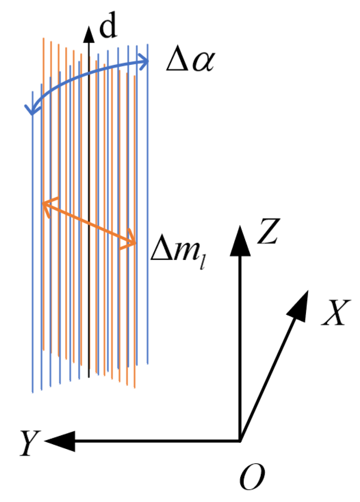
The artificial intermediate vector ${\mathbf{v}}_s$ is just used to construct the angle $\alpha$ to specify the relative location of the line on the red circle. Here, we note that $\mathbf{d}(\theta ,\varphi +\pi /2)$ is not vertical to $\mathbf{d}$ in the way how we define the direction vector. Figure 4 illustrates how the line’s position varies with $m_l$ and $\alpha$. $\Delta \alpha$ corresponds to movements on the red circle in Figure 2.

As pointed out in [41], the nonlinear minimal four-parameter representations for spatial lines usually have singularities. The proposed representation takes the distance from the origin to the line as one of the representation component, which makes it impossible to represent a line at infinite. Despite this singularity, it does not prevent the use of the proposed line representation in reconstruction and uncertainty analysis. In engineering practice, the cases of reconstructing lines at infinity will not occur basically.

2.3. Conversion between the Proposed Line Representation and the Plücker Line

Plücker lines have no singularities in representing spatial line and can be converted into other types of representation conveniently. Line transformation between different coordinate systems can also be easily represented in Plücker coordinates. These are the reasons why Plücker lines are widely employed. In this section, we derive the conversion between the proposed representation with Plücker lines, then we can also convert it into other types of representations easily.

In Plücker coordinates, a line is represented by six dependent variables; $\mathbf{d}$ corresponds to the direction part and $\mathbf{m}$ corresponds to the position part. As shown in Figure 5, ${\mathbf{L}}_1$, ${\mathbf{L}}_2$, and ${\mathbf{L}}_3$ correspond to $({\mathbf{m}}_1;\mathbf{d})$, $({\mathbf{m}}_2;\mathbf{d})$, and $({\mathbf{m}}_3;\mathbf{d})$, respectively. ${\mathbf{L}}_1$, ${\mathbf{L}}_2$ and ${\mathbf{L}}_3$ have the same direction $\mathbf{d}$. Since ${\mathbf{m}}_1$ and ${\mathbf{m}}_2$ are collinear, ${\mathbf{L}}_1$, ${\mathbf{L}}_2$ and the origin $\mathbf{O}$ are coplanar. As $\left|{\mathbf{m}}_1\right|=\left|{\mathbf{m}}_3\right|$, then ${\mathbf{L}}_1$ and ${\mathbf{L}}_3$ are tangents of the same 3D circle with a radius of $\left|{\mathbf{m}}_1\right|$. Accounting for the orthogonality between $\mathbf{m}$ and $\mathbf{d}$, and by forcing $\left|\mathbf{d}\right|=1$, a 3D line actually has four degrees of freedom. Similar to the Plücker line representation, the proposed spatial line representation has two parts; $\theta$ and $\varphi$ correspond to the directional part, $m_l$ and $\alpha$ correspond to the positional part.

2.3.1. From Plücker Line to the Proposed Representation

In homogeneous representation, ${\mathbf{L}}_{\mathbf{1}}=({\mathbf{m}}_1;{\mathbf{d}}_1)$ and ${\mathbf{L}}_2=(\lambda {\mathbf{m}}_2;\lambda {\mathbf{d}}_2)$ ($\lambda \ne 0$) represent the same line. In this paper, we force the norm of direction component to be 1: $\left|\mathbf{d}\right|=1$. This only prevents representing the lines at infinity(a Plücker line with $\mathbf{d}=\mathbf{0}$ is at infinity).

The direction $\mathbf{d}={(d_1,d_2,d_3)}^{\mathrm{T}}$ can be mapped to the unit sphere coordinate as $(\theta ,\varphi )$ directly:

$$\begin{array}{cc}\hfill \theta & =arccos{d}_3;\hfill \\ \hfill \varphi & =atan2(d_2,d_1),\hfill \end{array}$$

(11)

where $\theta \in [0,\pi )$ and $\varphi \in [-\pi ,\pi )$. In Plücker coordinates, the ratio of $\left|\mathbf{m}\right|$ and $\left|\mathbf{d}\right|$ implies the distance from the origin to the line. In our case, the distance is $\left|\mathbf{m}\right|$. Then

$$m_l=\left|\mathbf{m}\right|.$$

(12)

The closest point ${\mathbf{P}}_c$ on a Plücker line(with $\left|\mathbf{d}\right|=1$) to the origin can be represented by:

$${\mathbf{P}}_c=\mathbf{d}\times \mathbf{m}.$$

(13)

Therefore, the rotation angle $\alpha$ from ${\mathbf{v}}_s$ to ${\mathbf{OP}}_c$ about the axis $\mathbf{d}$ can be derived by:

$$\alpha =\left\{\begin{array}{cc}arccos\frac{{\mathbf{v}}_s^{\mathrm{T}}(\mathbf{d}\times \mathbf{m})}{\left|\mathbf{m}\right|}& {\mathbf{d}}^{\mathrm{T}}({\mathbf{v}}_s\times (\mathbf{d}\times \mathbf{m}))\ge 0\\ 2\pi -arccos\frac{{\mathbf{v}}_s^{\mathrm{T}}(\mathbf{d}\times \mathbf{m})}{\left|\mathbf{m}\right|}& {\mathbf{d}}^{\mathrm{T}}({\mathbf{v}}_s\times (\mathbf{d}\times \mathbf{m}))<0\end{array}\right..$$

(14)

Given $\mathbf{m}$ and $\mathbf{d}$, we can transform the redundant six-vector into a compact four-vector with certain physical meanings: $\theta$ and $\varphi$ imply the direction in sphere coordinate, $m_l=\left|\mathbf{m}\right|$ implies the minimum distance from the origin to the spatial line, $\alpha$ implies the location around the original.

2.3.2. From the Proposed Representation to Plücker Line

Conversely, given $(\theta ,\varphi ,m_l,\alpha )$, we can reconstruct the Plücker line by:

$$\begin{array}{cc}\hfill \mathbf{d}(\theta ,\varphi )& ={(sin\theta cos\varphi ,sin\theta sin\varphi ,cos\theta )}^{\mathrm{T}},\hfill \\ \hfill \mathbf{m}& =m_l\left(\mathbf{R}(\mathbf{d},\alpha ){\mathbf{v}}_s\right)\times \mathbf{d}(\theta ,\varphi ).\hfill \end{array}$$

(15)

2.4. Uncertainty Estimation and Visualization for Two-View Line Triangulation

2.4.1. Uncertainty Estimation

Given two observations of a 3D line in different image coordinates, as shown in Figure 1, the proposed compact representation of the line can be solved by triangulation:

$$\begin{array}{cc}\hfill \mathbf{L}(\theta ,\varphi ,m_l,\alpha )& =\mathbf{L}(\mathbf{m},\mathbf{d})\hfill \\ \hfill & =f({\mathbf{R}}_{wc}^1,{\mathbf{t}}_{wc}^1,{\mathbf{p}}_s^1,{\mathbf{p}}_e^1,{\mathbf{R}}_{wc}^2,{\mathbf{t}}_{wc}^2,{\mathbf{p}}_s^2,{\mathbf{p}}_e^2),\hfill \end{array}$$

(16)

where f is a constructed function for triangulation. In f, we first solve a Plücker line by (5) and then convert it into the proposed representation by Section 2.3.1. The input variables are poses of two cameras and endpoints of the observed line segments in each camera. Assume that all noises in input variables obey Gaussian distribution. The covariance matrix of the solved line $\mathbf{L}$ can be obtained by error propagation:

$${\Sigma }_{\mathbf{L}}=J_{\mathbf{L}}{\Sigma }_{in}{J}_{\mathbf{L}}^{\mathrm{T}},$$

(17)

where $J_{\mathbf{L}}$ is the Jacobian of f with respect to all input variables including poses and line segment detections, ${\Sigma }_{in}$ denotes the covariance matrix of all input variables. By constructing the function f, we can compute $J_{\mathbf{L}}$ numerically. To conveniently apply the proposed method directly to the work utilizing Plücker lines, we give the Jacobian of conversion from a Plücker line to the proposed representation in the Appendix A.

By analyzing the ${\Sigma }_{\mathbf{L}}$ we can evaluate the accuracy of the reconstructed line comprehensively. ${\Sigma }_{\mathbf{L}}$ can be blocked as:

$${\Sigma }_{\mathbf{L}}=\left(\begin{array}{cc}{\Sigma }_{\mathbf{dd}}& {\Sigma }_{\mathbf{dm}}\\ {\Sigma }_{\mathbf{md}}& {\Sigma }_{\mathbf{mm}}\end{array}\right).$$

(18)

To evaluate the accuracy of the reconstructed line, we can analyze ${\Sigma }_{\mathbf{dd}}$ and ${\Sigma }_{\mathbf{mm}}$ individually for orientation and position. The direction is a key attribution of 3D lines and badly reconstructed lines usually present large directional displacements. By separating the direction and position components, we are able to give an independent evaluation for direction and position. In addition, the uncertainty of a 3D line can be visualized by two ellipses by separating the directional and positional components, which is more intuitive and simple.

2.4.2. Uncertainty Visualization

Given the covariance matrix ${\mathbf{C}}_{\mathbf{x}}$ of a 2-dimensional vector $\mathbf{x}$, the confidence region is an ellipse. In this paper, we use 95% which means that the true value is in this ellipse with a statistical probability of 0.95. To solve a different confidence region, we can check the Chi-square distribution table. By projecting the ellipse to the axis of each component, we can get the confidence interval of each component with a certain probability. The smaller the fluctuation range of the confidence interval, the better the component is estimated.

2.4.3. Uncertainty Analysis

The orientational error tends to be much larger than the positional error in the presence of large levels of noise in image planes [32]. To determine the direction of a line, we can split it into three steps: Firstly, the normal vectors of projection planes ${\mathbf{n}}_c^1$ and ${\mathbf{n}}_c^2$ are computed. This step is affected by noise from camera calibration (in this work, we assume images are calibrated and ignore this item) and line segment extraction. Given two endpoints and constant Gaussian noise that causes displacement of line segment extraction, the computed normal vectors tend to be more accurate for longer line segments. This is the reason why most works ignore short line segments. Secondly, the normal vectors are transformed into the world coordinate system. This step is affected by noise on the rotation estimation of camera orientation. In pose estimation, images that are not well tracked should not be used to triangulate for 3D lines. Thirdly, the direction is computed by the cross product of two normal vectors in world coordinates. This step is affected by the relative orientation of normal vectors. The orientation differences of these two normal vectors come from relative movements vertical to the reference projection plane. Though relative movements along the reference projection plane do generate disparity, it contributes nothing to the direction determination. Degeneracy happens when relative movement is nearly along the projection plane. We can conclude that the quality of the estimated direction by triangulation is related to many factors: ego-motion of views, the accuracy of pose estimation and line segment extraction.

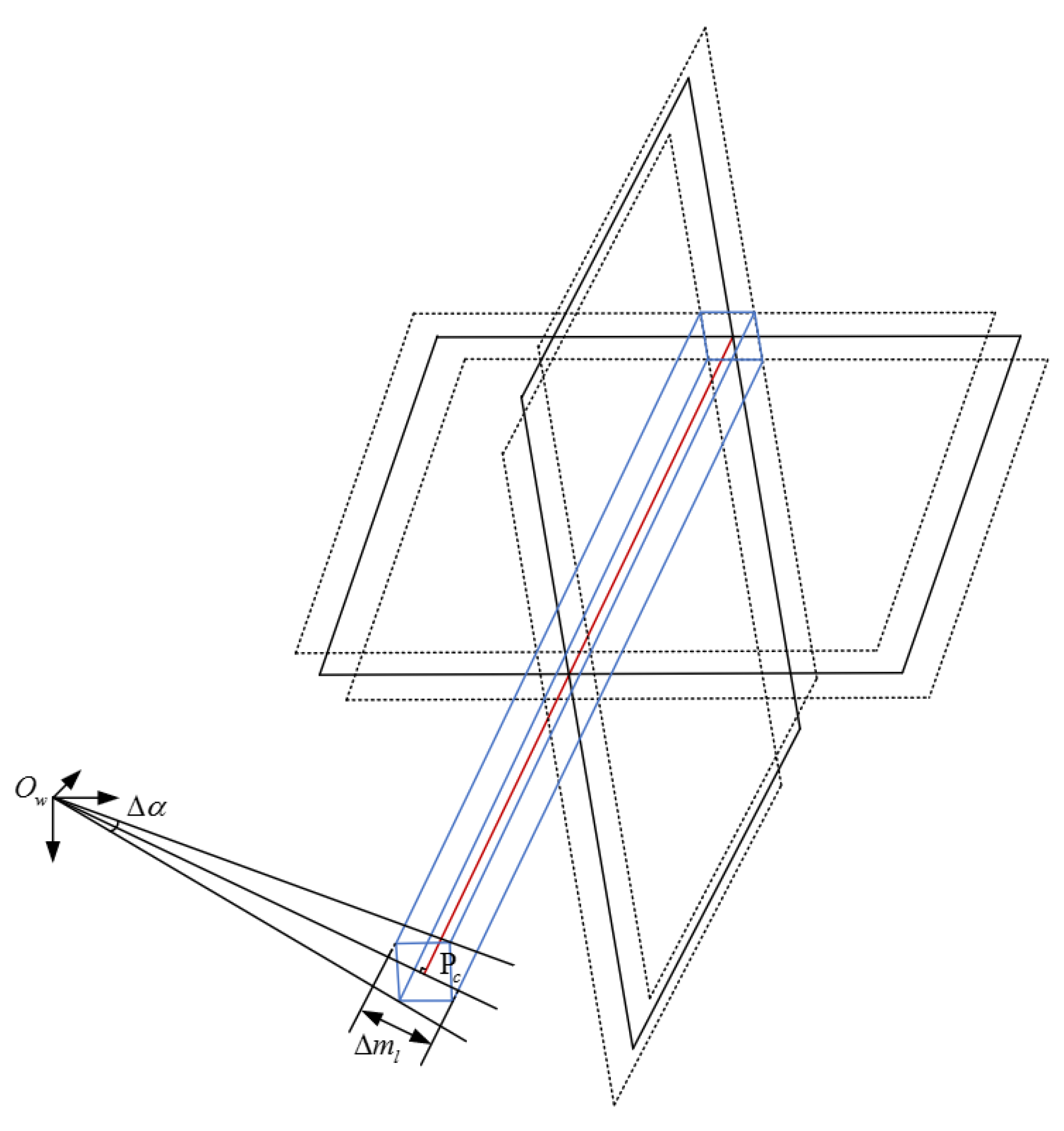
When discussing the positional error, we assume that the direction is known. An illustration of the distribution of the reconstructed line with fixed direction is given in Figure 6. A projection plane is determined by the camera’s optical center and the two endpoints of the line on the image plane. A line can be solved by intersecting two projection planes. Due to the error in camera position estimation and line detection, both projection planes are biased and finally lead to line reconstruction uncertainty. The cylinder indicated by the blue lines illustrates the distribution of the reconstructed line with a fixed direction. With fixed direction, line triangulation degenerates to a case similar to point triangulation. Both estimations only have one degree of freedom. In point triangulation, a good rule of thumb is that the angle between the rays determines the accuracy of reconstruction. While in our case of line reconstruction, the angle between the two projection planes determines the accuracy (size of the distribution). This also explains why further lines tend to preserve larger positional errors. The angle between the two projection planes decreases as the distance between the line and the camera centers increases. By intersecting the cylinder with a plane that passes through the origin and is perpendicular to the direction, the area of the section implies the uncertainty of the line position. $\Delta \alpha$ and $\Delta m_l$ in Figure 6 implies the position accuracy in the proposed representation.

2.5. Uncertainty Update by Multiple Triangulations

Each time a new observation of the spatial line is obtained, a new constraint equation is imported and contributes to decreasing the uncertainty of reconstruction. Each pair of observations yield a sub-uncertainty. Uncertainty of multi-view reconstruction is a fusion of these sub-uncertainties. Given a prior estimation ${\mathbf{D}}_p\sim N\left({\mathbf{x}}_p,{\Sigma }_p\right)$ and a new noisy estimation ${\mathbf{D}}_n\sim N\left({\mathbf{x}}_n,{\Sigma }_n\right)$, the posterior estimation ${\mathbf{D}}_m\sim N\left({\mathbf{x}}_m,{\Sigma }_m\right)$ can be obtained by multiplying ${\mathbf{D}}_p$ and ${\mathbf{D}}_n$:

$$\begin{array}{cc}\hfill {\mathbf{x}}_m& ={\Sigma }_p{({\Sigma }_p+{\Sigma }_n)}^{-1}{\mathbf{x}}_n+{\Sigma }_n{({\Sigma }_p+{\Sigma }_n)}^{-1}{\mathbf{x}}_p,\hfill \\ \hfill {\Sigma }_m& ={\Sigma }_p{({\Sigma }_p+{\Sigma }_n)}^{-1}{\Sigma }_n.\hfill \end{array}$$

(19)

Each time we get a new observation of the line, we can update the uncertainty with (19) incrementally.

3. Results

We have performed experimental validation of the proposed uncertainty analysis. Experiments on simulation data are designed to validate the correctness of the uncertainty estimation of line reconstruction. Experiments on synthetic and real-world dataset provide results of the application in map culling. We have carried out all experiments with an Intel Core i7-7700K (8 cores @ 4.20GHz) and 16Gb RAM. Section 3.1 is implemented in MATLAB(R2017A), Section 3.2 and Section 3.3 are implemented in C++.

3.1. Experiments on Simulation Data

3.1.1. Experiment on Simulation Data to Validate and Visualize Uncertainty of Two-View Line Triangulation

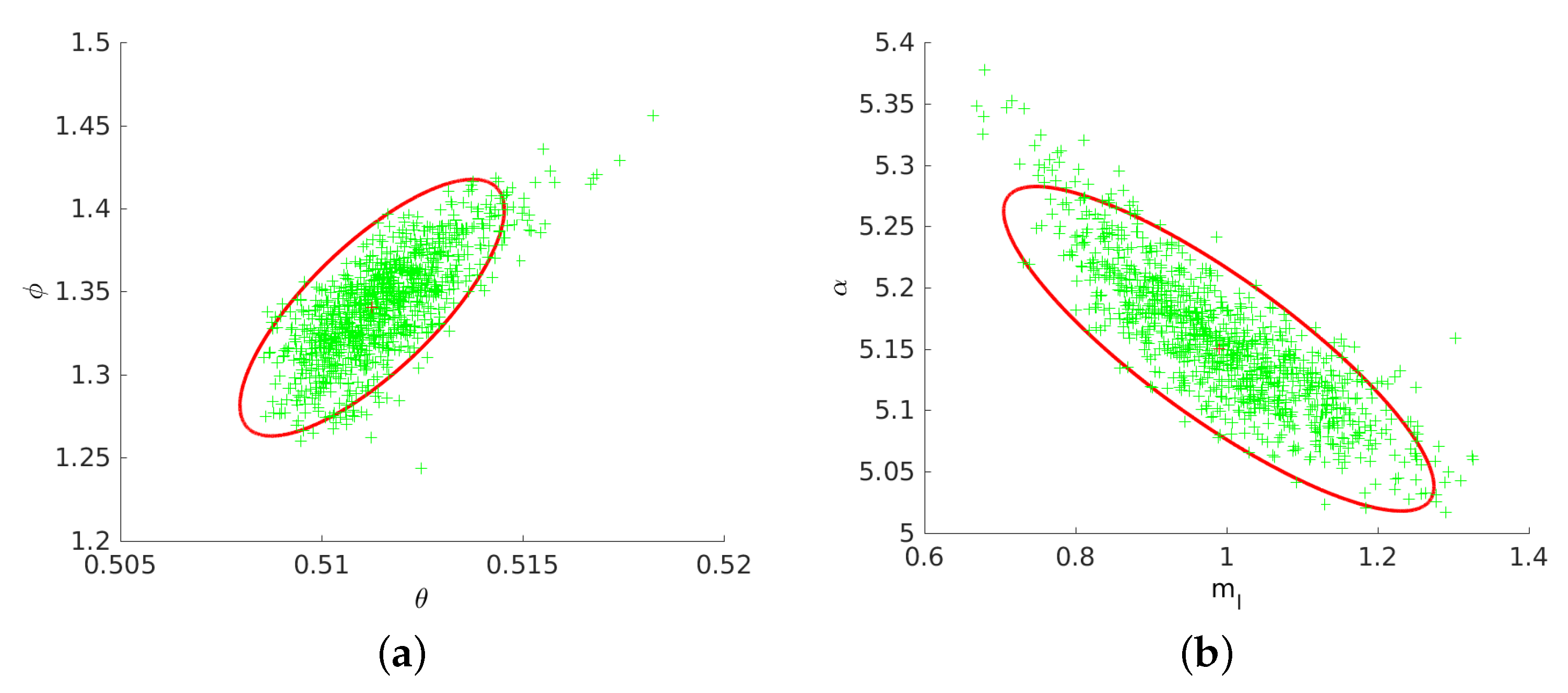
To validate and visualize the uncertainty of a reconstructed line by two-view triangulation, a randomly generated 3D line is projected to two cameras with known poses and intrinsic matrices. In our experiment, we set intrinsic parameters: $f_x=f_y=1000$, $c_x=640$, $c_y=360$. For each trial, every component of rotation is added with Gaussian noise with a standard deviation of 0.02 deg; every component of translation is added with Gaussian noise with a standard deviation of 0.02 m; for line segment extraction, each axis of endpoints is added with Gaussian noises with a standard deviation of 0.5 pixels. This synthetic noisy data is used to solve a 3D line in the proposed representation. The test is repeated 1000 times for reliability. Figure 7 illustrates the results of the Monte Carlo test and uncertainty visualization. Figure 7a shows the estimated 95% confidence region and noisy estimations of $(\theta ,\varphi )$. Figure 7b shows the estimated 95% confidence region and noisy estimations of $(m_l,\alpha )$. The statistical results verify the correctness of the uncertainty estimation in the proposed line representation.

3.1.2. Experiment on Simulation Data to Validate and Visualize Uncertainty of Multi-View Line Reconstruction

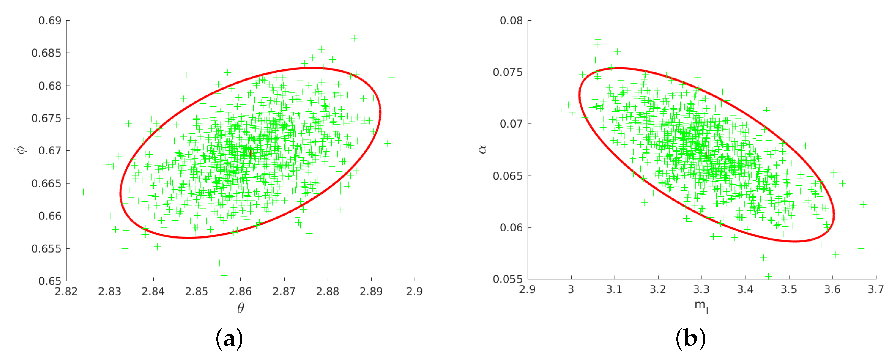
As described in Section 2.5, the uncertainty of multi-view line reconstruction can be extended by two-view triangulation. In this section, we use three views as an example. Given a line projected to three cameras, we can obtain an estimation of the spatial line by (7). Three observations can construct three triangulations. Each triangulation contributes to an estimated uncertainty. The uncertainty of the final estimation is obtained by fusing these sub-uncertainties. Uncertainty of line reconstruction from more than three views can also be obtained in this manner. To validate the uncertainty estimation of thee-view line reconstruction, a randomly generated spatial line is projected to three randomly generated cameras. Camera intrinsic parameters are: $f_x=f_y=1000$, $c_x=640$, $c_y=360$. Gaussian noises are added to camera poses and endpoints of observations. The standard deviation of Gaussian noise on three rotation angles is all set to $0.05deg$. The standard deviation of Gaussian noise on three camera translation components is all set to 0.005m. The standard deviation of Gaussian noise on the endpoints of the line segment is set to 0.3 pixels. For each trial, a spatial line is estimated with this noisy input. The test is repeated 1000 times for reliability. Figure 8 shows the result of Monte Carlo test on uncertainty estimation of three-view line reconstruction. Figure 8a shows the estimated 95% confidence region and noisy estimations of direction. Figure 8b shows the estimated 95% confidence region and noisy estimations of momentum. The results validate the correctness of fusion-based uncertainty estimation for three-view reconstruction. Thus it can also be extended to uncertainty estimation of multi-view reconstruction.

3.1.3. Experiment on Simulation Data to Validate Uncertainty Decrease by Multiple Observations

To illustrate the fusion process of uncertainty, a randomly generated 3D line is projected to multiple images. Similar to the last synthetic experiment, noise with known standard deviation is added to all input variables. Every following observation is used to triangulate with the first observation, the estimated line parameters and uncertainty are incrementally updated. As illustrated in Figure 9a, every red ellipse denotes the estimated 95% confidence region of $(\theta ,\varphi )$ by one triangulation; the green ellipse denotes the final 95% confidence region of $(\theta ,\varphi )$ by incremental fusion. Figure 9b shows the case for $(m_l,\alpha )$ in the proposed compact representation. The blue “*” represents the ground truth and the green “*” represents the finally estimated $(\theta ,\varphi )$ or $(m_l,\alpha )$ by incremental fusion. Figure 9c shows the decrease of 95% confidence interval of every component in the proposed compact representation by the incremental update. A more accurate estimation with smaller uncertainty can be obtained by importing more observations. When the confidence interval of each parameter is smaller than the respective thresholds, the line is thought to be well-reconstructed.

3.2. Experiment on Synthetic Image Sequence

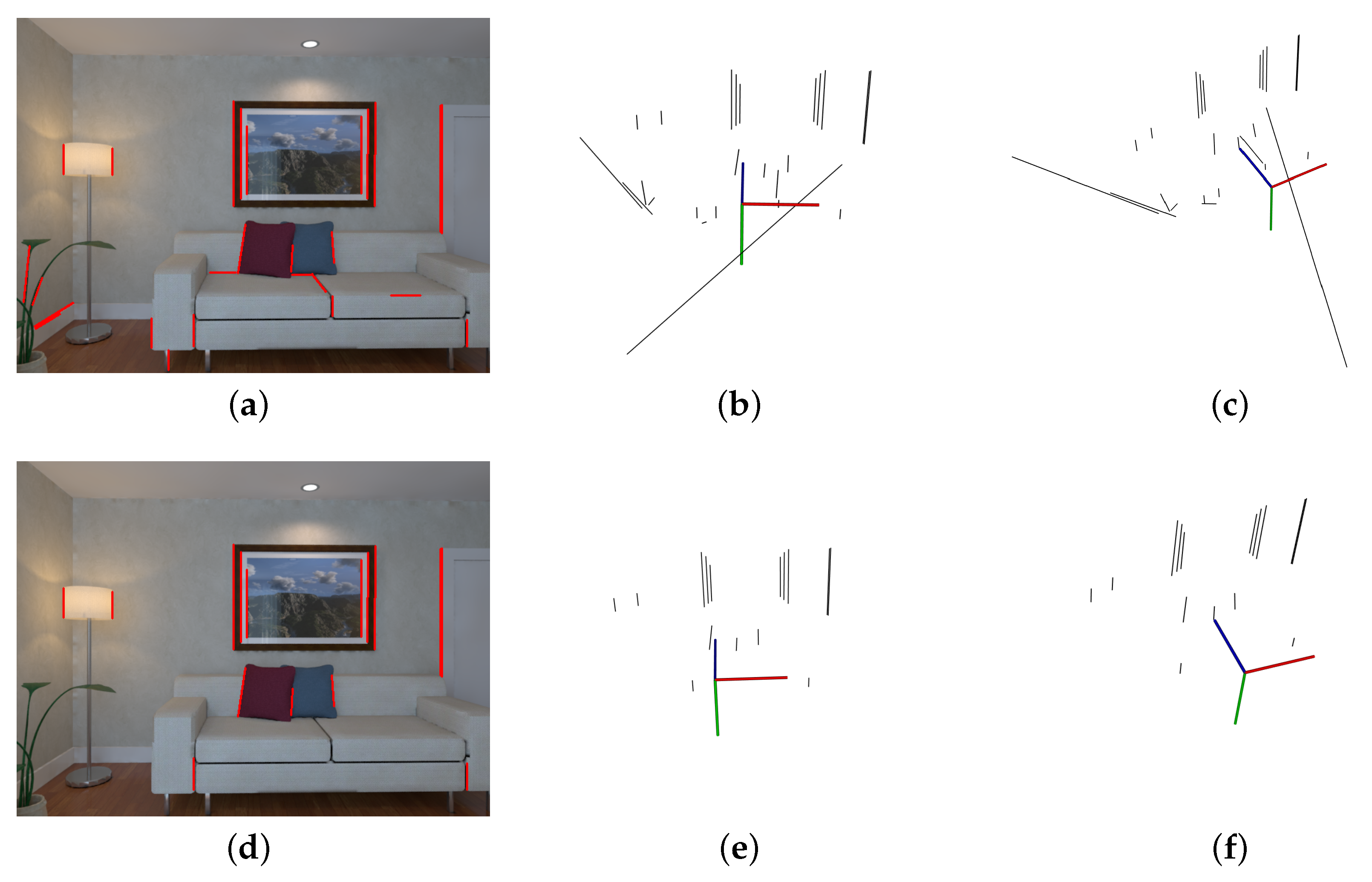
To validate the efficiency of the proposed uncertainty analysis in outlier rejection, we also test the proposed method on a synthetic image sequence. The experiment is performed on “Living Room 2” from ICL-NUIM dataset, which provides ground truth trajectory and depth maps. The former 90 frames are used to perform an incremental mapping. The first frame is set to be the reference frame and the detected line segments in the reference frame are tracked in the following 89 frames (after 90 frames, the scene is totally changed, line segments on the reference frame are no longer tracked. No new observations are acquired to update the lines’ estimation and uncertainty). The line segments are extracted by the LSD algorithm proposed in [43]. Line segments are matched by combining the LBD [44] and relaxed epiolar constraint introduced in [16]. Once a line segment is tracked in the following images, a 3D line and its uncertainty are estimated by triangulation with the reference image. If the uncertainty is too large, the current estimation is abandoned; otherwise, the current estimation is used to update prior estimation. In this experiment, Gaussian noises are added to rotation(standard deviation ${\delta }_r$ = 0.02 rad for each axis) and translation(standard deviation ${\delta }_t$ = 5 $\times {10}^{-4}$ m for each axis). We assume that the standard deviation of the endpoints is 0.5 pixels. The ground truths of line segments in the first frame are obtained by reprojecting the 2D line segment to 3D as the depths were known. Two items were computed for each estimation: the angular bias between the estimated line and the ground truth line; the mean of distances from endpoints to the ground truth line. The former item indicates the orientation accuracy and the later item indicates the positional accuracy. If the angular error is less than 10 deg and mean distance is less than 0.05 m, an estimation is regarded as well-reconstructed.

We compared results of outlier rejection only with reprojection error and incorporating reprojection error with uncertainty. In reprojection error based outlier rejection, the reprojection error for an observation is defined as the sum of distances between line segment endpoints to the projected line. We set a threshold on mean reprojection error ${\tau }_{rep}$ = 1 pixel, which is a very strict condition. However, as illustrated in Figure 10b,c, some lines are apparently inconsistent with the scene. In uncertainty based outlier rejection, we set thresholds on each component: ${\tau }_{\theta }$ = 0.7 rad, ${\tau }_{\varphi }$ = 0.7 rad, ${\tau }_{m_l}$ = 0.2 m, ${\tau }_{\alpha }$ = 0.7 rad (in a normal distribution, the length of the 95% confidence interval is approximately four times the standard deviation. To ensure that the standard deviation of each angular component does not exceed 10 degrees, we set these angle thresholds to 40 degrees (0.7 in radius)). As illustrated in Figure 10e,f, no such lines left by adding the uncertainty based outlier rejection.

Table 1. 3D line map quality after outlier rejection with different methods.

Outlier Rejection Method	Mean Directional Error (deg)	Mean Distance Error (m)	Good Line Ratio
Reprojection error	21.73	9.05	57.69%
Reprojection error + Uncertainty	0.76	0.01	93.33%

reports the quality of the 3D line map after outlier rejection. The mean angular error and distance error is computed for quality comparison. The good line ratio denotes the percentage of the well-reconstructed line in the culled map. After outlier rejection by reprojection error, 26 lines are left but only 15 lines are well-reconstructed. In this sequence, the camera presents frequent on-spot rotations, which results in many lines with large uncertainties. When an additional rejection by uncertainty is utilized, 15 lines are left and 14 lines are well-reconstructed. By incorporating reprojection error and uncertainty, a 3D line map with higher quality is obtained.

3.3. Experiment on rEal-World Image Sequence

To demonstrate the application of the proposed uncertainty analysis in line reconstruction of real-world scenarios, we also conducted experiments on the Merton I dataset (data available: www.robots.ox.ac.uk/~vgg/data/). The Merton I dataset is a real-world dataset which contains three images of an Oxford University building and provides line segment matching across views. The proposed uncertainty analysis is used to detect those poorly localized lines with small reprojection errors. Firstly, the camera poses and sparse point reconstruction is computed by COLMAP [45,46], a general-purpose Structure-from-Motion (SfM) and Multi-View Stereo (MVS) pipeline with a graphical and command-line interface. Secondly, camera covariance matrixes are estimated by the method proposed in [30]. Then, a 3D line map is generated and the associated uncertainty is estimated by the proposed uncertainty fusion method. The camera poses with uncertainty and line tracks across images are used as input. Finally, the line map is culled. In map culling, we present results with and without uncertainty based rejection.

3.3.1. Implementation Details

In the selection of line segment, we only use line segments longer than 20 pixels. In uncertainty based method, each line segment detected in the reference image is initialized with a freely given estimation with large uncertainty: $\theta =\pi /4$, $\varphi =\pi /4$, $m_l=1.0$, $\alpha =\pi /4$, and

$${\Sigma }_L=\left[\begin{array}{cc}{10}^6& \\ & {10}^6& \\ & & {10}^6\\ & & & {10}^6\end{array}\right].$$

(20)

In uncertainty based line map culling, thresholds are set on $\theta$, $\varphi$, and $\alpha$. Scale ambiguity always exists in monocular projection. If the scale is unknown, the estimated translation vectors, $m_l$ and other distance-related parameters are all up to an unknown scale. It is not suitable to set a fixed threshold on $m_l$ because it varies with scale. In this experiment, the poses are estimated by structure from motion and the scale is unknown. We do not set a threshold on $m_l$ to reject outliers. In our implementation, ${\tau }_{\theta }=0.7$ rad, ${\tau }_{\varphi }=0.7$ rad, and ${\tau }_{\alpha }=0.7$ rad, which implies that the 95% confidence interval for each angular component is 0.7 in radius.

3.3.2. Experimental Results

Figure 11 shows an example of the uncertainty fusion and visualization on the real-world dataset. In Figure 11a, for example, line segments are labeled as A, B, C, and D. Taking A as an example, Figure 11b,c show the uncertainty visualization of orientation and position, respectively. Each red ellipse denotes the 95% confidence region of an estimation. The blue ellipse illustrates the confidence region after fusion.

Table 2. The 95% confidence interval length of each component for line segment A, B, C, and D.

Line Segment	$\mathbf{\Delta }\mathit{\theta }$ (rad)	$\mathbf{\Delta }\mathit{\varphi }$ (rad)	$\mathbf{\Delta }{\mathit{m}}_{\mathit{l}}$	$\mathbf{\Delta }\mathit{\alpha }$ (rad)
A	0.089	0.012	21.11	0.047
B	0.084	0.010	21.06	0.047
C	0.526	0.158	159.21	0.674
D	0.123	0.013	25.17	0.045

reports lengths of the final 95% confidence region for these four line segments. By comparing the direction uncertainty of the line segments A and B on the $\theta$ and $\varphi$ components, we can conclude that longer line segments can be better estimated. As for the line segment C, though C is much longer than A and B, C presents a larger direction uncertainty since the camera centers all lie in about a horizontal plane, which is in line with our previous analysis. Only the component of camera motion that is vertical to the reference projection plane reduces the direction uncertainty. The further line D has a larger positional uncertainty compared with A, which is also consistent with our previous analysis.

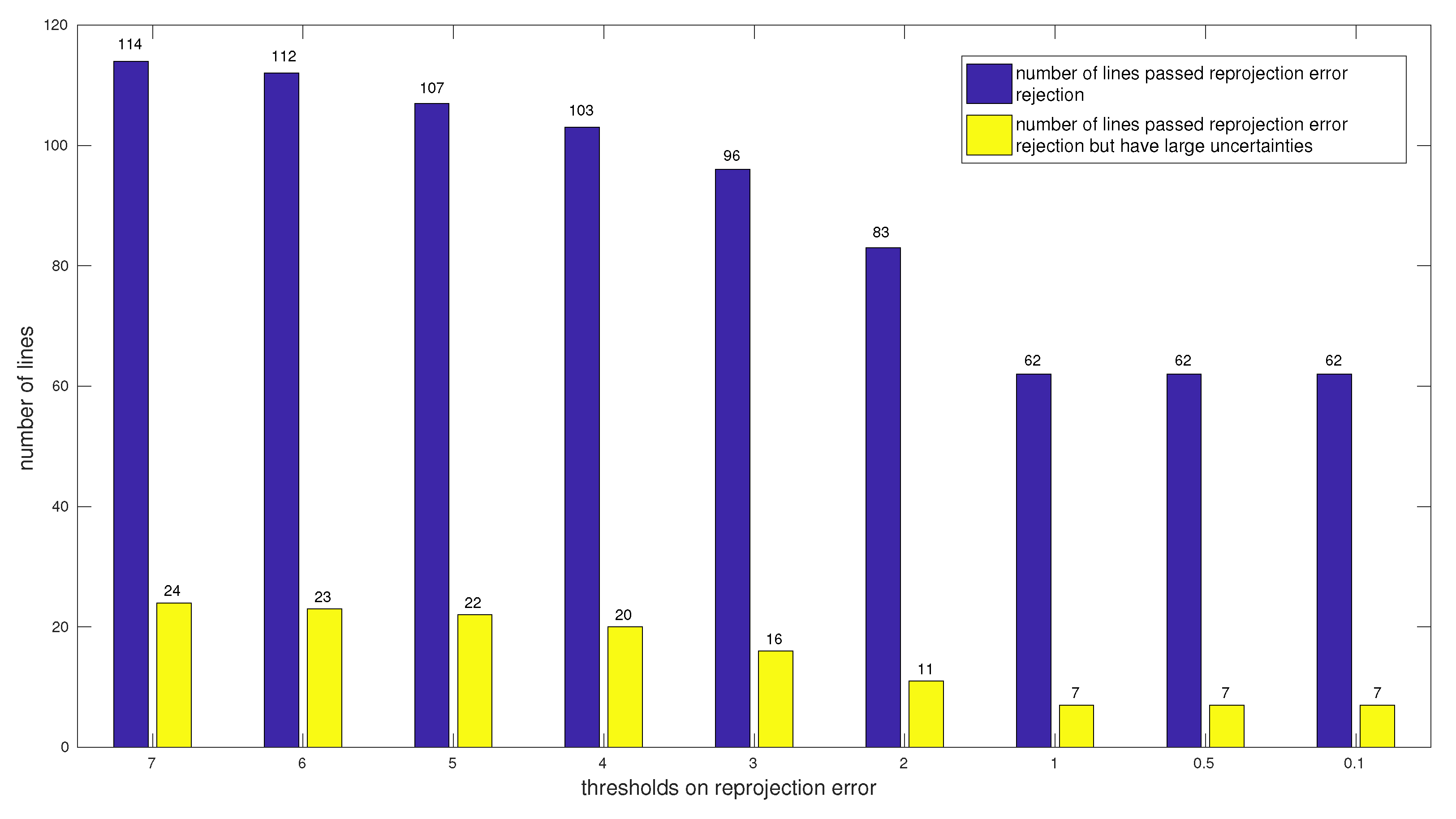
Figure 12 reports the number of lines that presented large uncertainties under different reprojection error thresholds. By varying the threshold of reprojection error, we counted the number of lines that passed the reprojection error rejection but presented large uncertainties. As illustrated in Figure 12, nine tests were conducted and the reprojection error threshold was reduced from 7 to 0.1 pixels. In each test, the blue bar denotes the number of lines that passed the reprojection error rejection, and the yellow bar denotes the number of lines that passed the reprojection error rejection but failed in the uncertainty rejection. By setting a smaller threshold on reprojection error, the reconstructed lines with large uncertainties can be reduced to some extent. However, lines with small reprojection errors can still be reconstructed inaccurately. Although the reprojection error was set to 0.1 pixels, there were still seven lines presenting large uncertainties. The results show that small reprojection errors do not guarantee the accuracy of the reconstructed lines when nearly degenerate cases happen. An additional test is required to reject these lines.

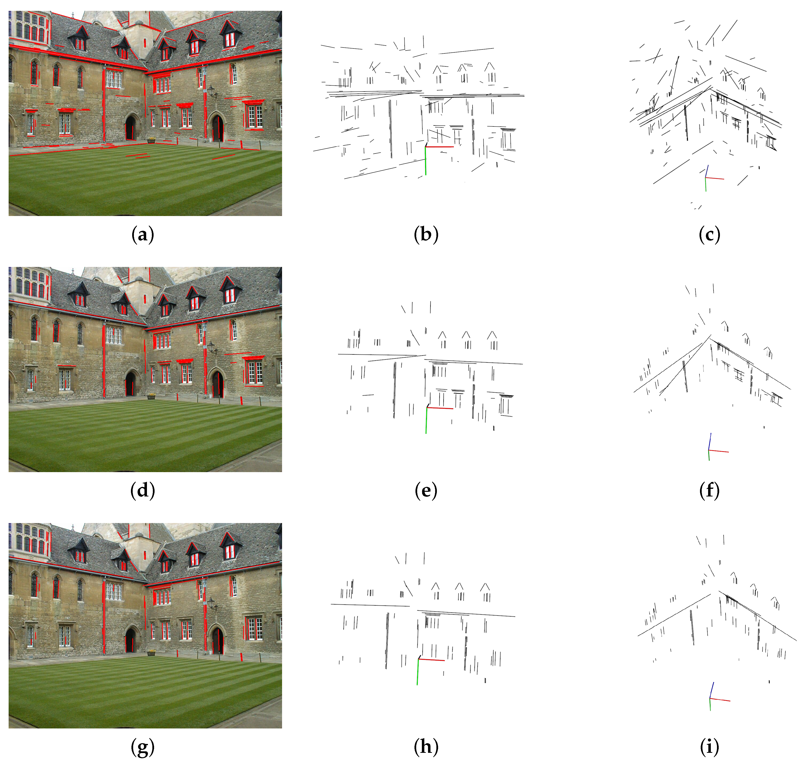
Figure 13 shows the reconstructed 3D line map and culled maps by different methods. The first row shows the 3D line map without map culling. The second row shows the results after reprojection error based map culling. The last row shows the results culled by reprojection error and uncertainty. The first column denotes the corresponding line segments in the first image. The last two columns show the corresponding 3D line maps from different views. As noted in the description of the dataset, there are still some mismatches because camera centers all lie in about a horizontal plane. This results in some badly reconstructed lines in Figure 13b,c. Mismatches cause inconsistency in multi-view stereo and present large reprojection errors. As illustrated in Figure 13e,f, the badly reconstructed lines due to mismatches can be rejected by setting a threshold on reprojection error(here we set ${\tau }_{rep}=2$ pixels, few lines are left if we set the same threshold on reprojection error as Section 3.2). The proposed uncertainty analysis originates from two-view triangulation and holds the assumption that line matches are correct, thus it is not robust to mismatches. By integrating the reprojection error and uncertainty, both inaccurate lines due to mismatches and unreliable lines from insufficient effective ego-motion can be rejected. As showed in Figure 13 h,i, a 3D line map consistent to the scene structure is obtained. By comparing Figure 13d,g, we can figure out which lines are rejected by the uncertainty rejection. The common characteristic of these lines is that they are nearly coplanar with camera movements, which results in estimations with large uncertainties.

In existing line reconstruction work, the reprojection error has always been the golden rule to ensure accuracy. however, the reprojection error is an indirect reflection of the accuracy in the image plane and fails in two-view triangulation. In the proposed uncertainty analysis, the accuracy is directly evaluated by the positional and orientational uncertainty of the line in 3D. Map culling can be robust to degenerate cases by adding the proposed uncertainty analysis.

4. Conclusions

This paper proposed a compact representation of 3D lines and applied it to the uncertainty analysis of line reconstruction. A spatial line is represented by a distance and three angles in the proposed representation. The advantage of this representation is that there is no parameter redundancy and each component has a clear physical meaning, which is well suited for uncertainty analysis. Based on the proposed representation, the quality of a line reconstructed from two-view triangulation can be measured by the confidence interval of each parameter. Furthermore, we extended the uncertainty estimation of the two-view triangulation to multi-view reconstruction. The proposed method is capable of distinguishing those poorly reconstructed lines from nearly degenerate cases. The main concern of our work is to provide a quantitative evaluation of reconstruction accuracy and detect the nearly degenerate cases of line reconstruction, especially under limited view range and baseline. By integrating the reprojection error and the proposed uncertainty analysis, we are capable of culling badly reconstructed from mismatches and nearly degenerate cases. The proposed method can be used in reconstructing high-quality 3D line models and localization. Our future work will apply the proposed method to visual odometry with line segments.

References

1. Bartoli, A.; Sturm, P.F. Structure-from-motion using lines: Representation, triangulation, and bundle adjustment. Comput. Vis. Image Underst. 2005, 100, 416–441. [Google Scholar] [CrossRef] [Green Version]
2. Zhang, L.; Koch, R. Structure and motion from line correspondences: Representation, projection, initialization and sparse bundle adjustment. J. Vis. Commun. Image Represent. 2014, 25, 904–915. [Google Scholar] [CrossRef]
3. Taylor, C.J.; Kriegman, D.J. Structure and motion from line segments in multiple images. IEEE Trans. Pattern Anal. Mach. Intell. 1995, 17, 1021–1032. [Google Scholar] [CrossRef]
4. Hofer, M.; Wendel, A.; Bischof, H. Incremental Line-based 3D Reconstruction using Geometric Constraints. In Proceedings of the British Machine Vision Conference (BMVC), Bristol, UK, 9–13 September 2013. [Google Scholar]
5. Gomez-Ojeda, R.; Zuñiga-Noël, D.; Moreno, F.A.; Scaramuzza, D.; Gonzalez-Jimenez, J. PL-SLAM: A Stereo SLAM System through the Combination of Points and Line Segments. arXiv 2017, arXiv:1705.09479. [Google Scholar] [CrossRef] [Green Version]
6. Pumarola, A.; Vakhitov, A.; Agudo, A.; Sanfeliu, A.; Moreno-Noguer, F. PL-SLAM: Real-time monocular visual SLAM with points and lines. In Proceedings of the 2017 IEEE International Conference on Robotics and Automation (ICRA), Singapore, 29 May–3 June 2017; pp. 4503–4508. [Google Scholar]
7. Gee, A.P.; Mayol-Cuevas, W. Real-time model-based SLAM using line segments. In Proceedings of the International Symposium on Visual Computing, Lake Tahoe, NV, USA, 6–8 November 2006; Springer: Berlin, Germany, 2006; pp. 354–363. [Google Scholar]
8. Smith, P.; Reid, I.D.; Davison, A.J. Real-Time Monocular SLAM with Straight Lines. In Proceedings of the British Machine Vision Conference, Edinburgh, UK, 4–7 September 2006; pp. 17–25. [Google Scholar]
9. Marzorati, D.; Matteucci, M.; Migliore, D.; Sorrenti, D.G. Integration of 3D Lines and Points in 6DoF Visual SLAM by Uncertain Projective Geometry. In Proceedings of the 2007 European Conference on Mobile Robots, Freiburg, Germany, 19–21 September 2007; pp. 96–101. [Google Scholar]
10. Zuo, X.; Xie, X.; Liu, Y.; Huang, G. Robust visual SLAM with point and line features. In Proceedings of the 2017 IEEE/RSJ International Conference on Intelligent Robots and Systems (IROS), Vancouver, BC, Canada, 24–28 September 2017; pp. 1775–1782. [Google Scholar]
11. Gomez-Ojeda, R.; Briales, J.; Gonzalez-Jimenez, J. PL-SVO: Semi-direct Monocular Visual Odometry by combining points and line segments. In Proceedings of the 2016 IEEE/RSJ International Conference on Intelligent Robots and Systems (IROS), Daejeon, Korea, 9–14 October 2016; pp. 4211–4216. [Google Scholar]
12. He, Y.; Zhao, J.; Guo, Y.; He, W.; Yuan, K. PL-VIO: Tightly-Coupled Monocular Visual–Inertial Odometry Using Point and Line Features. Sensors 2018, 18, 1159. [Google Scholar] [CrossRef] [PubMed] [Green Version]
13. Ok, A.Ö.; Wegner, J.D.; Heipke, C.; Rottensteiner, F.; Sörgel, U.; Toprak, V. Accurate Reconstruction of Near-Epipolar Line Segments from Stereo Aerial Images. Photogramm. Fernerkund. Geoinf. 2012, 2012, 341–354. [Google Scholar] [CrossRef]
14. Hofer, M.; Maurer, M.; Bischof, H. Improving Sparse 3D Models for Man-Made Environments Using Line-Based 3D Reconstruction. In Proceedings of the 2014 2nd International Conference on 3D Vision, Tokyo, Japan, 8–11 December 2014; Volume 1, pp. 535–542. [Google Scholar]
15. Jain, A.; Kurz, C.; Thormählen, T.; Seidel, H.P. Exploiting Global Connectivity Constraints for Reconstruction of 3D Line Segments from Images. In Proceedings of the Twenty-Third IEEE Conference on Computer Vision and Pattern Recognition, San Francisco, CA, USA, 13–18 June 2010; pp. 1586–1593. [Google Scholar]
16. Hofer, M.; Maurer, M.; Bischof, H. Efficient 3D scene abstraction using line segments. Comput. Vis. Image Underst. 2017, 157, 167–178. [Google Scholar] [CrossRef]
17. Sugiura, T.; Torii, A.; Okutomi, M. 3D surface reconstruction from point-and-line cloud. In Proceedings of the 2015 International Conference on 3D Vision (3DV), Lyon, France, 19–22 October 2015; pp. 264–272. [Google Scholar]
18. Hartley, R.; Zisserman, A. Multiple view geometry in computer vision. Kybernetes 2004, 30, 1865–1872. [Google Scholar]
19. Schmude, N.v. Visual Localization with Lines. Ph.D. Thesis, University of Heidelberg, Heidelberg, Germany, 2017. [Google Scholar]
20. Zhou, H.; Zhou, D.; Peng, K.; Fan, W.; Liu, Y. SLAM-based 3D Line Reconstruction. In Proceedings of the 2018 13th World Congress on Intelligent Control and Automation (WCICA), Changsha, China, 4–8 July 2018; pp. 1148–1153. [Google Scholar] [CrossRef]
21. Zhou, H.; Fan, H.; Peng, K.; Fan, W.; Zhou, D.; Liu, Y. Monocular Visual Odometry Initialization With Points and Line Segments. IEEE Access 2019, 7, 73120–73130. [Google Scholar] [CrossRef]
22. Felzenszwalb, P.F.; Huttenlocher, D.P. Efficient Graph-Based Image Segmentation. Int. J. Comput. Vis. 2004, 59, 167–181. [Google Scholar] [CrossRef]
23. Donoser, M. Replicator Graph Clustering. In Proceedings of the British Machine Vision Conference (BMVC), Bristol, UK, 9–13 September 2013; pp. 38.1–38.11. [Google Scholar]
24. Förstner, W.P.; Wrobel, B. Photogrammetric Computer Vision; Springer International Publishing: Cham, Switzerland, 2016; Volume 11. [Google Scholar] [CrossRef] [Green Version]
25. Blostein, S.D.; Huang, T.S. Error analysis in stereo determination of 3-d point positions. IEEE Trans. Pattern Anal. Mach. Intell. 1988, 9, 765. [Google Scholar] [CrossRef] [PubMed]
26. Rivera-Rios, A.H.; Shih, F.L.; Marefat, M. Stereo Camera Pose Determination with Error Reduction and Tolerance Satisfaction for Dimensional Measurements. In Proceedings of the IEEE International Conference on Robotics & Automation, Barcelona, Spain, 18–22 April 2005. [Google Scholar]
27. Morris, D.D. Gauge Freedoms and Uncertainty Modeling for Three-dimensional Computer Vision. Ph.D. Thesis, Carnegie Mellon University, Pittsburgh, PA, USA, 2001. [Google Scholar]
28. Park, S.Y.; Subbarao, M. A multiview 3D modeling system based on stereo vision techniques. Mach. Vis. Appl. 2005, 16, 148–156. [Google Scholar] [CrossRef]
29. Grossmann, E.; Santos-Victor, J. Uncertainty analysis of 3D reconstruction from uncalibrated views. Image Vis. Comput. 2000, 18, 685–696. [Google Scholar] [CrossRef]
30. Polic, M.; Förstner, W.; Pajdla, T. Fast and Accurate Camera Covariance Computation for Large 3D Reconstruction. In Computer Vision—ECCV 2018; Springer International Publishing: Berlin, Germany, 2018; pp. 697–712. [Google Scholar]
31. Wolff, L.B. Accurate measurement of orientation from stereo using line correspondence. In Proceedings of the CVPR ’89: IEEE Computer Society Conference on Computer Vision and Pattern Recognition, San Diego, CA, USA, 4–8 June 1989; pp. 410–415. [Google Scholar] [CrossRef]
32. Balasubramanian, R.; Swaminathan, S.D.K. Error analysis in reconstruction of a line in 3-D from two arbitrary perspective views. Int. J. Comput. Math. 2001, 78, 191–212. [Google Scholar] [CrossRef]
33. Lu, Y. Visual Navigation for Robots in Urban and Indoor Environments. Ph.D. Thesis, Chang’an University, Xi’an, China, 2015. [Google Scholar]
34. Heuel, S.; Forstner, W. Matching, reconstructing and grouping 3D lines from multiple views using uncertain projective geometry. In Proceedings of the IEEE Computer Society Conference on Computer Vision & Pattern Recognition, Kauai, HI, USA, 8–14 December 2001. [Google Scholar]
35. Weng, J.; Huang, T.S.; Ahuja, N. Motion and structure from line correspondences; closed-form solution, uniqueness, and optimization. IEEE Trans. Pattern Anal. Mach. Intell. 1992, 14, 318–336. [Google Scholar] [CrossRef] [Green Version]
36. Seo, Y.; Hong, K.S. Sequential reconstruction of lines in projective space. In Proceedings of the 13th International Conference on Pattern Recognition, Vienna, Austria, 25–29 August 1996; Volume 1, pp. 503–507. [Google Scholar]
37. Pottmann, H.; Hofer, M.; Odehnal, B.; Wallner, J. Line geometry for 3D shape understanding and reconstruction. In Proceedings of the European Conference on Computer Vision, Prague, Czech Republic, 11–14 May 2004; Springer: Berlin, Germany, 2004; pp. 297–309. [Google Scholar]
38. Ronda, J.I.; Gallego, G.; Valdés, A. Camera autocalibration using plucker coordinates. In Proceedings of the IEEE International Conference on Image Processing 2005, Genova, Italy, 14 September 2005; Volume 3, pp. III–800. [Google Scholar]
39. Ohwovoriole, M.S. An Externsion of Screw Theory and Its Application to the Automation of Industrial Assemblies. Ph.D. Thesis, Mechanical Engineering. Standford University, Stanford, CA, USA, 1980. [Google Scholar]
40. Krantz, S.G. Handbook of Complex Variables; Birkhäuser: Boston, MA, USA, 1999. [Google Scholar]
41. Roberts, K.S. A new representation for a line. In Proceedings of the CVPR ’88: The Computer Society Conference on Computer Vision and Pattern Recognition, Ann Arbor, MI, USA, 5–9 June 1988; pp. 635–640. [Google Scholar] [CrossRef]
42. Heuel, S. Uncertain Projective Geometry: Statistical Reasoning For Polyhedral Object Reconstruction (Lecture Notes in Computer Science); Springer: Berlin/Heidelberg, Germany, 2004. [Google Scholar]
43. Gioi, R.G.V.; Jakubowicz, J.; Morel, J.M.; Randall, G. LSD: A Fast Line Segment Detector with a False Detection Control. IEEE Trans. Pattern Anal. Mach. Intell. 2010, 32, 722–732. [Google Scholar] [CrossRef] [PubMed]
44. Zhang, L.; Koch, R. An efficient and robust line segment matching approach based on LBD descriptor and pairwise geometric consistency. J. Vis. Commun. Image Represent. 2013, 24, 794–805. [Google Scholar] [CrossRef]
45. Schönberger, J.L.; Zheng, E.; Pollefeys, M.; Frahm, J.M. Pixelwise View Selection for Unstructured Multi-View Stereo. In Proceedings of the European Conference on Computer Vision (ECCV), Amsterdam, The Netherlands, 11–14 October 2016. [Google Scholar]
46. Schönberger, J.L.; Frahm, J.M. Structure-from-Motion Revisited. In Proceedings of the Conference on Computer Vision and Pattern Recognition (CVPR), Las Vegas, NV, USA, 1–26 June 2016. [Google Scholar]
Figure 1. A 3D line is projected to two cameras. The line can be determined by intersecting two projection planes.
Applsci 10 01096 g001
Figure 2. Specify a certain line by v s and α . The lines with fixed direction d and distance m l to the origin are all tangent of a circle(colored in red) with a radius of m l . A point P c on the circle corresponds to a certain line.
Applsci 10 01096 g002
Figure 3. The variation of line direction with the fluctuation of θ and ϕ . The fluctuation Δ θ is added to θ and Δ ϕ is added to ϕ . The cone indicates the fluctuation of direction with Δ θ and Δ ϕ .
Applsci 10 01096 g003
Figure 4. The variation of line position(with fixed direction d ) with the fluctuation of m l and α . The fluctuation Δ m l is added to m l and Δ α is added to α .
Applsci 10 01096 g004
Figure 5. Correspondences of 3D lines and Plücker lines with the same d but different m .
Applsci 10 01096 g005
Figure 6. Uncertainty of line reconstruction with fixed direction by triangulation. The cylinder region illustrates the uncertainty region, which depends on the biases of the planes and the angle between the planes.
Applsci 10 01096 g006
Figure 7. Monte Carlo test to validate the uncertainty estimation of line triangulation. (a) The red ellipse denotes the estimated 95% confidence region of ( θ , ϕ ) . Red “+” denotes the ground truth. Each green “+” represents a noisy estimation of ( θ , ϕ ) . (b) The red ellipse denotes the estimated 95% confidence region of ( m l , α ) . Red “+” denotes the ground truth. Each green “+” represents a noisy estimation of ( m l , α ) .
Applsci 10 01096 g007
Figure 8. Monte Carlo test to validate the uncertainty estimation of three-view line reconstruction. (a) The red ellipse denotes the estimated 95% confidence region of ( θ , ϕ ) . Red “+” denotes the ground truth. Each green “+” represents a noisy estimation of ( θ , ϕ ) . (b) The red ellipse denotes the estimated 95% confidence region of ( m l , α ) . Red “+” denotes the ground truth. Each green “+” represents a noisy estimation of ( m l , α ) .
Applsci 10 01096 g008
Figure 9. Uncertainty fusion by multiple triangulations. (a) Red ellipses denote uncertainty estimated by each triangulation, the green ellipse denotes the final uncertainty after fusion. The blue “*” represents the ground truth of d and the green “*” represents the finally estimated d . (b) The same case for m as described in (a). (c) The 95% confidence interval length of θ , ϕ , m l and α decrease along with more and more observations.
Applsci 10 01096 g009
Figure 10. Outlier rejection with and without uncertainty. The first row shows reconstructed lines only with reprojection error based outlier rejection: (a) reconstructed line segments on the reference frame; (b) front view of reconstructed 3D lines. (c) Side view of reconstructed 3D lines. The second row shows reconstructed lines that pass reprojection error and uncertainty tests: (d) reconstructed line segments on the reference frame; (e) front view of reconstructed 3D lines. (f) Side view of reconstructed 3D lines.
Applsci 10 01096 g010
Figure 11. Example of uncertainty estimation, fusion and visualization for line reconstruction. By fusing these noisy estimations, a posterior estimation with smaller uncertainty can be obtained. The uncertainty of direction and position are visualized by 95% confidence region. (a) Four example line segments are labelled on the image, the corresponding confidence interval length of each component are reported in Table 2. (b) Uncertainty estimation and fusion of direction components for A. Δ θ and Δ ϕ correspond to 95% confidence interval lengths of θ and ϕ , respectively. (c) Uncertainty estimation and fusion of positional components for A. Δ m l and Δ α are the confidence interval lengths of positional components m l and α .
Applsci 10 01096 g011
Figure 12. The number of lines passed reprojection error rejection and the number of lines passed reprojection error rejection but have large uncertainties at different reprojection error thresholds.
Applsci 10 01096 g012
Figure 13. Reconstructed 3D line map and map culling with different methods. The first column shows the mapped line segments in the image and the later two columns show the corresponding 3D line map from different viewpoints. In the first row, no lines are culled. In the second row, the line map is culled by reprojection error. In the third row, the line map is firstly culled by reprojection error and then culled by uncertainty.
Applsci 10 01096 g013