A New Method of Fuzzy Support Vector Machine Algorithm for Intrusion Detection

Abstract
1. Introduction
- Our paper proposed a new fuzzy membership function which can effectively distinguish the noises and SVs distributed on the boundary based on SVDD. SVs are given larger weight coefficients while noises are given smaller coefficients. In this way, our method avoids imperfection of FSVM based on the distance between a sample and its cluster center. Such a fuzzy membership function structure method is more in line with reality.
- The method proposed in our paper uses the hyperplane, which passes through the cluster center and takes the line of two cluster centers as the normal vector to replace each cluster center. This is in accordance with the geometric principle of SVM. In other words, two hyperplanes with maximum space are used to separate the training samples. Therefore, using the hyperplane in class to replace the cluster center can better approximate the actual situation.
- Our method is more efficient, especially for anomaly-based IDS with high real-time requirements. In our method, the noises and outliers are identified by a sphere with minimum volume while containing the maximum of the samples. Some uncontributed vectors are eliminated by pre-extracting the boundary vector set containing the support vectors. This reduces the number of training samples and speeds up the training. It is important that IDS speed up detection as much as possible by reducing computation and storage.
2. Previous Work
3. Methodology Based on SVDD
3.1. Analysis
3.2. Support Vector Data Description
3.3. Design Fuzzy Membership Function
4. Experimental Evaluation
4.1. The Experimental Data
4.2. The Experimental Performance
5. Conclusions
Author Contributions
Funding
Acknowledgments
Conflicts of Interest
References
- Khraisat, A.; Gondal, I.; Vamplew, P.; Kamruzzaman, J.; Alazab, A. A novel Ensemble of Hybrid Intrusion Detection System for Detecting Internet of Things Attacks. Electronics 2019, 8, 1210. [Google Scholar] [CrossRef]
- Chung, Y.; Kim, N.; Park, C.; Lee, J. Improved Neighborhood Search for Collaborative Filtering. Int. J. Fuzzy Log. Intell. Syst. 2018, 18, 29–40. [Google Scholar] [CrossRef]
- Vapnik, V.N.; Chervonenkis, A.Y. On the uniform convergence of relative frequencies of events to their probabilities. Theory Probab. Its Appl. 1971, 16, 264–279. [Google Scholar] [CrossRef]
- Liu, Y.; Xu, Z.; Li, C.G. Online semi-supervised support vector machine. Inf. Sci. 2018, 439, 125–141. [Google Scholar] [CrossRef]
- Nan, S.; Sun, L.; Chen, B.; Lin, Z.; Toh, K.A. Density-dependent quantized least squares support vector machine for large data sets. IEEE Trans. Neural Netw. Learn. Syst. 2017, 28, 94–106. [Google Scholar] [CrossRef] [PubMed]
- Kim, J.S.; Jeong, J.S. Pattern Recognition of Ship Navigational Data Using Support Vector Machine. Int. J. Fuzzy Log. Intell. Syst. 2015, 15, 268–276. [Google Scholar] [CrossRef]
- Maza, S.; Touahria, M. Feature selection algorithms in intrusion detection system: A survey. KSII Trans. Internet Inf. Syst. 2018, 12, 5079–5099. [Google Scholar]
- Bostani, H.; Sheikhan, M. Hybrid of binary gravitational search algorithm and mutual information for feature selection in intrusion detection systems. Soft Comput. 2017, 21, 2307–2324. [Google Scholar] [CrossRef]
- Xiao, X.; Zhang, S.; Mercaldo, F.; Hu, G.; Sangaiah, A.K. Android malware detection based on system call sequences and LSTM. Multimed. Tools Appl. 2019, 78, 3937–3999. [Google Scholar] [CrossRef]
- Jiang, G.; Chen, H.; Ungureanu, C.; Yoshihira, K. Multiresolution abnormal trace detection using varied-length n-grams and automata. IEEE Trans. Syst. Man Cybern. Part C Appl. Rev. 2007, 37, 86–97. [Google Scholar] [CrossRef]
- Laszka, A.; Abbas, W.; Sastry, S.S.; Vorobeychik, Y.; Koutsoukos, X. Optimal thresholds for intrusion detection systems. In Proceedings of the Symposium and Bootcamp on the Science of Security (HotSos’16:), Pittsburgh, PA, USA, 20–21 April 2016; pp. 72–81. [Google Scholar]
- Tan, K.M.; Maxion, R.A. “Why 6?” Defining the operational limits of Stide, an anomaly-based intrusion detector. In Proceedings of the 2002 IEEE Symposium on Security and Privacy, Berkeley, CA, USA, 12–15 May 2002; pp. 188–201. [Google Scholar]
- Alarifi, S.S.; Wolthusen, S.D. Detecting anomalies in IaaS environments through virtual machine host system call analysis. In Proceedings of the 2012 International Conference for Internet Technology and Secured Transactions, London, UK, 10–12 December 2012; pp. 211–218. [Google Scholar]
- Xue, B.; Cervante, L.; Shang, L.; Browne, W.N.; Zhang, M. A multi-objective particle swarm optimisation for filter-based feature selection in classification problems. Connect. Sci. 2012, 24, 91–116. [Google Scholar] [CrossRef]
- Qu, G.; Hariri, S.; Yousif, M. A new dependency and correlation analysis for features. IEEE Trans. Knowl. Data Eng. 2005, 17, 1199–1207. [Google Scholar] [CrossRef]
- Luo, B.; Xia, J. A novel intrusion detection system based on feature generation with visualization strategy. Expert Syst. Appl. 2014, 41, 4139–4147. [Google Scholar] [CrossRef]
- Nauman, M.; Azam, N.; Yao, J. A three-way decision making approach to malware analysis using probabilistic rough sets. Inf. Sci. 2016, 374, 193–209. [Google Scholar] [CrossRef]
- Ahmed, M.; Mahmood, A.N.; Hu, J. A survey of network anomaly detection techniques. J. Netw. Comput. Appl. 2016, 60, 19–31. [Google Scholar] [CrossRef]
- Pektas, A.; Acarman, T. Deep learning for effective Android malware detection using API call graph embeddings. Soft Comput. 2019, 24, 1027–1043. [Google Scholar] [CrossRef]
- Forrest, S.; Hofmeyr, S.A.; Somayaji, A. The Evolution of System-Call Monitoring. The evolution of system-call monitoring. In Proceedings of the 24th Annual Computer Security Applications Conference, Anaheim, CA, USA, 8–12 December 2008; pp. 418–430. [Google Scholar]
- Forrest, S.; Beauchemin, C.; Somayaji, A. Computer immunology. Immunol. Rev. 2007, 216, 176–197. [Google Scholar] [CrossRef]
- Haxhibeqiri, J.; Moerman, I.; Hoebeke, J. Low overhead scheduling of LoRa transmissions for improved scalability. IEEE Internet Things J. 2018, 6, 3097–3109. [Google Scholar] [CrossRef]
- Xu, L.; Zhang, D.; Alvarez, M.A.; Morales, J.A.; Ma, X.; Cavazos, J. Dynamic android malware classification using graph-based representations. In Proceedings of the 2016 IEEE 3rd International Conference on Cyber Security and Cloud Computing, Beijing, China, 25–27 June 2016; pp. 220–231. [Google Scholar]
- Patgiri, R. HFil: A High Accuracy Bloom Filter. In Proceedings of the IEEE 21st International Conference on High Performance Computing and Communications, Zhangjiajie, China, 10–12 August 2019; pp. 1–12. [Google Scholar]
- Ye, Q.; Wu, X.; Yan, B. An Intrusion Detection Approach Based on System Call Sequences and Rules Extraction. In Proceedings of the IEEE 2010 International Conference on E-business and Information System Security (EBISS), Wuhan, China, 22–23 May 2010; pp. 1–4. [Google Scholar]
- Glass-Vanderlan, T.R.; Iannacone, M.D.; Vincent, M.S.; Bridges, R.A. A Survey of Intrusion Detection Systems Leveraging Host Data. ACM Comput. Surv. 2018, 52, 1–40. [Google Scholar]
- Zhang, H.; Xiao, X.; Mercaldo, F.; Ni, S.; Martinelli, F.; Sangaiah, A.K. Classification of ransomware families with machine learning based on N-gram of opcodes. Future Gener. Comput. Syst. 2019, 90, 211–212. [Google Scholar] [CrossRef]
- Laurén, S.; Rauti, S.; Leppänen, V. Diversification of system calls in linux kernel. In Proceedings of the 16th International Conference on Computer Systems and Technologies, Dublin, Ireland, 25 June 2015; pp. 284–291. [Google Scholar]
- Durán, F.; Salaün, G. Robust and reliable reconfiguration of cloud applications. J. Syst. Softw. 2016, 122, 524–537. [Google Scholar] [CrossRef]
- Bigyan, P. Thesis-Generating Knowledgebase of Common Behavior and Workflow Patterns for Secure Systems. Master’ Thesis, East Carolina University, Greenville, NC, USA, 2018. [Google Scholar]
- Kumar, G.R.; Mangathayaru, N.; Narasimha, G. An approach for intrusion detection using text mining techniques. In Proceedings of the International Conference on Engineering & MIS (ICEMIS), Istanbul, Turkey, 24–26 September 2015; pp. 63–74. [Google Scholar]
- Dimjašević, M.; Atzeni, S.; Ugrina, I.; Rakamaric, Z. Evaluation of android malware detection based on system calls. In Proceedings of the ACM on International Workshop on Security and Privacy Analytics, New Orleans, LA, USA, 11–12 March 2016; pp. 1–8. [Google Scholar]
- Nissim, N.; Lapidot, Y.; Cohen, A.; Elovici, Y. Trusted system-calls analysis methodology aimed at detection of compromised virtual machines using sequential mining. Knowl. Based Syst. 2018, 153, 147–175. [Google Scholar] [CrossRef]
- Zuzcak, M.; Sochor, T.; Zenka, M. Intrusion detection system for home windows based computers. KSII Trans. Internet Inf. Syst. 2019, 13, 4706–4726. [Google Scholar]
- Wang, Q.H.; Ouyang, X.Q.; Zhan, J.C. A classification algorithm based on data clustering and data reduction for intrusion detection system over big data. KSII Trans. Internet Inf. Syst. 2019, 13, 3714–3732. [Google Scholar]
- Howard, A.G.; Zhu, M.; Chen, B.; Kalenichenko, D.; Wang, W.; Weyand, T.; Andreetto, M.; Adam, H. MobileNets: Efficient Convolutional Neural Networks for Mobile Vision Applications. Comput. Sci. 2017, 5, 16–29. [Google Scholar]
- Pan, J.; Liu, S.; Sun, D.; Zhang, J.; Liu, Y.; Ren, J.; Li, Z.; Tang, J.; Lu, H.; Tai, Y.-W.; et al. Learning Dual Convolutional Neural Networks for Low-Level Vision. In Proceedings of the IEEE Conference on Computer Vision and Pattern Recognition (CVPR), Salt Lake, UT, USA, 18–23 June 2018; pp. 3070–3079. [Google Scholar]
- Wang, X.; Girshick, R.; Gupta, A.; He, K. Non-local neural networks. In Proceedings of the IEEE Conference on Computer Vision and Pattern Recognition (CVPR), Salt Lake, UT, USA, 18–23 June 2018; pp. 7794–7803. [Google Scholar]
- Collobert, R.; Weston, J. A unified architecture for natural language processing: Deep neural networks with multitask learning. In Proceedings of the 25th International Conference on Machine Learning, Helsinki, Finland, 7–8 July 2008; pp. 160–167. [Google Scholar]
- Hirschberg, J.; Manning, C.D. Advances in natural language processing. Science 2015, 349, 261–266. [Google Scholar] [CrossRef]
- Goldberg, Y. A Primer on Neural Network Models for Natural Language Processing. Comput. Sci. 2015, 4, 67–77. [Google Scholar] [CrossRef]
- Shah, B.; Trivedi, B.H. Artificial Neural Network based Intrusion Detection System: A Survey. Int. J. Comput. Appl. 2012, 39, 13–18. [Google Scholar] [CrossRef]
- Staudemeyer, R.C.; Omlin, C.W. Evaluating performance of long short-term memory recurrent neural networks on intrusion detection data. In Proceedings of the South African Institute for Computer Scientists and Information Technologists Conference (SAICSIT 13), East London, South Africa, 7–9 October 2013; p. 218. [Google Scholar]
- Kim, G.; Yi, H.; Lee, J.; Paek, Y.; Yoon, S. LSTM-Based System-Call Language Modeling and Robust Ensemble Method for Designing Host-Based Intrusion Detection Systems. arXiv 2016, arXiv:1611.01726. [Google Scholar]
- LeCun, Y.; Bengio, Y.; Hinton, G. Deep learning. Nature 2015, 521, 436–444. [Google Scholar] [CrossRef]
- Chen, L.; Sultana, S.; Sahita, R. HeNet: A Deep Learning Approach on Intel circled Processor Trace for Effective Exploit Detection. arXiv 2018, arXiv:1801.02318. [Google Scholar]
- Chen, Q.; Luley, R.; Wu, Q.; Bishop, M.; Linderman, R.W.; Qiu, Q. AnRAD: A neuromorphic anomaly detection framework for massive concurrent data streams. IEEE Trans. Neural Netw. Learn. Syst. 2018, 29, 1622–1636. [Google Scholar] [CrossRef] [PubMed]
- Naseer, S.; Saleem, Y. Enhanced network intrusion detection using deep convolutional neural networks. Ksii Trans. Internet Inf. Syst. 2018, 12, 5159–5178. [Google Scholar]
- Ambusaidi, M.A.; He, X.; Nanda, P.; Tan, Z. Building an intrusion detection system using a filter-based feature selection algorithm. IEEE Trans. Comput. 2016, 65, 2986–2998. [Google Scholar] [CrossRef]
- Creech, G.; Hu, J. A semantic approach to host-based intrusion detection systems using contiguous and discontiguous system call patterns. IEEE Trans. Comput. 2014, 63, 807–819. [Google Scholar] [CrossRef]
- Khreich, W.; Murtaza, S.S.; Hamou-Lhadj, A.; Talhi, C. Combining heterogeneous anomaly detectors for improved software security. J. Syst. Softw. 2018, 137, 415–429. [Google Scholar] [CrossRef]
- Abdlhamed, M.; Lifayat, K.; Shi, Q.; Hurst, W. Intrusion prediction systems. In Information Fusion for Cyber-Security Analytics; Springer International Publishing: Cham, Germany, 2019; pp. 1358–1363. [Google Scholar]
- Lv, S.; Wang, J.; Yang, Y.; Liu, J. Intrusion prediction with system-call sequence-to-sequence model. IEEE Access. 2018, 6, 1358–1363. [Google Scholar] [CrossRef]
- Zhang, Z.; Peng, Z.; Zhou, Z. The Study of Intrusion Prediction Based on HsMM. In Proceedings of the Asia Pacific Services Computing Conference, 2008 (APSCC ‘08), Yilan, Taiwan, 9–12 December 2008; pp. 1358–1363. [Google Scholar]
- Watson, M.R.; Marnerides, A.K.; Mauthe, A.; Hutchison, D. Malware detection in cloud computing infrastructures. IEEE Trans. Dependable Secur. Comput. 2016, 13, 192–205. [Google Scholar] [CrossRef]
- Xie, M.; Hu, J.; Slay, J. Evaluating host-based anomaly detection systems: Application of the one-class SVM algorithm to ADFA-LD. In Proceedings of the 2014 11th International Conference on Fuzzy Systems and Knowledge Discovery (FSKD’14), Xiamen, China, 19–21 August 2014; pp. 978–982. [Google Scholar]
- Kang, Q.; Shi, L.; Zhou, M.; Wang, X.; Wu, Q.; Wei, Z. A distance-based weighted under sampling scheme for support vector machines and its application to imbalanced classification. IEEE Trans. Neural Netw. Learn. Syst. 2017, 99, 4152–4165. [Google Scholar]
- Chandra, M.A.; Bedi, S.S. Survey on SVM and their application in image classification. Int. J. Inf. Technol. 2018, 3, 1–11. [Google Scholar] [CrossRef]
- Alabdallah, A.; Awad, M. Using weighted support vector machine to address the imbalanced classes problem of intrusion detection system. KSII Trans. Internet Inf. Syst. 2019, 12, 5143–5158. [Google Scholar]
- Abe, S. Fuzzy support vector machines for multilabel classification. Pattern Recognit. 2015, 48, 2110–2117. [Google Scholar] [CrossRef]
- Huang, H.P.; Liu, Y.H. Fuzzy support vector machines for pattern recognition and data mining. Int. J. Fuzzy Syst. 2002, 4, 826–835. [Google Scholar]
- Deepak, G.; Bharat, R.; Parashjyoti, B. A fuzzy twin support vector machine based on information entropy for class imbalance learning. Neural Comput. Appl. 2018, 31, 7153–7164. [Google Scholar]
- Chen, S.G.; Wu, X.J. A new fuzzy twin support vector machine for pattern classification. Int. J. Mach. Learn. Cybern. 2018, 9, 1553–1564. [Google Scholar] [CrossRef]
- Wang, Y.; Wang, S.; Lai, K.K. A new fuzzy support vector machine to evaluate credit risk. IEEE Trans. Fuzzy Syst. 2006, 13, 820–831. [Google Scholar] [CrossRef]
- An, W.; Liang, M. Fuzzy support vector machine based on within-class scatter for classification problems with outliers or noises. Neurocomputing 2013, 110, 101–110. [Google Scholar] [CrossRef]
- Jiang, X.; Yi, Z.; Lv, J.C. Fuzzy SVM with a new fuzzy membership function. Neural Comput. Appl. 2006, 15, 268–276. [Google Scholar] [CrossRef]
- Lin, C.F.; Wan, S.D. Fuzzy support vector machines. IEEE Trans. Neural Netw. 2002, 13, 464–471. [Google Scholar]
- Xiang, Z.; Xiao-Ling, X.; Guang-You, X.U. Fuzzy Support Vector Machine Based on Affinity among Samples. J. Softw. 2006, 17, 951–958. [Google Scholar]
- Zhang, X. Using class-center vectors to build support vector machines. In Proceedings of the IEEE Signal Processing Society Workshop, Madison, WI, USA, 25 August 1999; pp. 3–11. [Google Scholar]
- Warrender, C.; Forrest, S.; Pearlmutter, B. Detecting intrusions using system calls: Alternative data models. In Proceedings of the IEEE Symposium on Security and Privacy, Oakland, CA, USA, 14 May 1999; pp. 133–145. [Google Scholar]


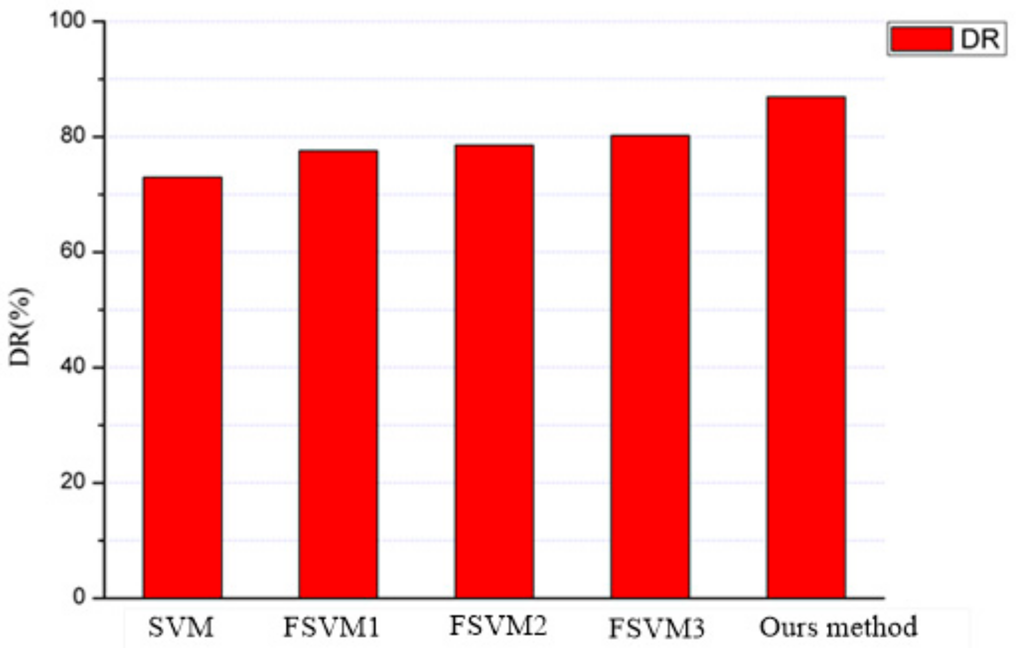
| Algorithm | Detection Rate (%) | Missing Rate (%) | False Alarm Rate (%) |
|---|---|---|---|
| SVM | 79.88% | 20.12% | 8.64% |
| FSVM1 | 83.71% | 16.29% | 7.30% |
| FSVM2 | 85.56% | 14.44% | 8.17% |
| FSVM3 | 86.20% | 13.80% | 6.92% |
| Our algorithm | 92.63% | 7.37% | 6.16% |
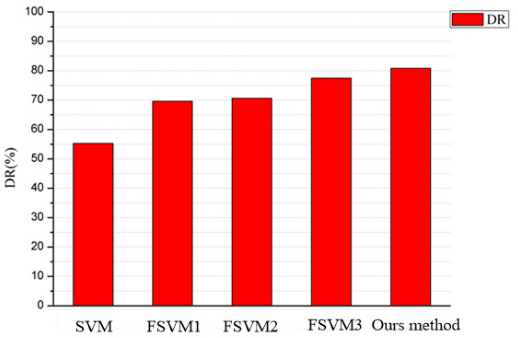
| Algorithm | Detection Rate (%) | Missing Rate (%) | False Alarm Rate (%) |
|---|---|---|---|
| SVM | 61.53% | 38.47% | 10.14% |
| FSVM1 | 76.92% | 23.08% | 9.57% |
| FSVM2 | 76.92% | 23.08% | 8.17% |
| FSVM3 | 83.21% | 16.23% | 6.92% |
| Our algorithm | 84.61% | 15.39% | 4.51% |
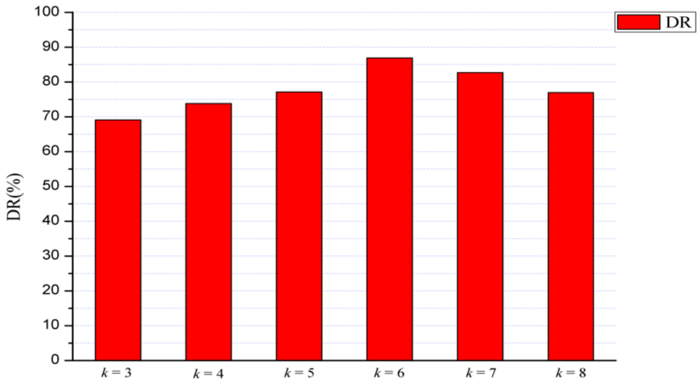
| Our Method | k = 3 | k = 4 | k = 5 | k = 6 | k = 7 | k = 8 |
|---|---|---|---|---|---|---|
| Detection rate | 78.30% | 83.25% | 86.31% | 92.63% | 88.26% | 83.27% |
| Missing rate | 21.70% | 16.75% | 13.69% | 7.37% | 11.74% | 16.73% |
| False alarm rate | 11.76% | 11.32% | 10.60% | 6.16% | 6.30% | 7.56% |
| Our Method | k = 3 | k = 4 | k = 5 | k = 6 | k = 7 | k = 8 |
|---|---|---|---|---|---|---|
| Detection rate | 77.22% | 82.45% | 85.37% | 84.61% | 86.46% | 81.37% |
| Missing rate | 22.78% | 17.55% | 14.63% | 15.39% | 13.54% | 18.63% |
| False alarm rate | 14.67% | 12.12% | 11.68% | 4.51% | 6.85% | 9.53% |
| Algorithm | Detection Rate (%) | Missing Rate (%) | False Alarm Rate (%) |
|---|---|---|---|
| N.bayes | 65.11% | 30.12% | 4.77% |
| Uniqueness | 39.1% | 55.3% | 2.30% |
| Hybrid Markov | 45.6% | 40.22% | 14.26% |
| Bayes1-step Markov | 62.6% | 33.3% | 4.1% |
| IPMA | 45.05% | 47.37% | 7.58% |
| Sequence matching | 36.7% | 58.2% | 5.91% |
| Compression | 33.9% | 50.1% | 16% |
| Closeness | 76.5% | 19.2% | 4.3% |
| Our algorithm | 92.63% | 7.37% | 6.16% |
| Algorithm | Detection Rate (%) | Missing Rate (%) | False Alarm Rate (%) |
|---|---|---|---|
| N.bayes | 63.88% | 32.12% | 4.00% |
| Uniqueness | 37.4% | 60.3% | 2.30% |
| Hybrid Markov | 45.3% | 40.44% | 14.26% |
| Bayes1-step Markov | 67.3% | 30.8% | 1.9% |
| IPMA | 40.63% | 42.37% | 17% |
| Sequence matching | 35.9% | 60.2% | 3.9% |
| Compression | 29.7% | 50.5% | 19.8% |
| Closeness | 75.2% | 20.1% | 4.7% |
| Our algorithm | 84.61% | 15.39% | 4.51% |
© 2020 by the authors. Licensee MDPI, Basel, Switzerland. This article is an open access article distributed under the terms and conditions of the Creative Commons Attribution (CC BY) license (http://creativecommons.org/licenses/by/4.0/).
Share and Cite
Liu, W.; Ci, L.; Liu, L. A New Method of Fuzzy Support Vector Machine Algorithm for Intrusion Detection. Appl. Sci. 2020, 10, 1065. https://doi.org/10.3390/app10031065
Liu W, Ci L, Liu L. A New Method of Fuzzy Support Vector Machine Algorithm for Intrusion Detection. Applied Sciences. 2020; 10(3):1065. https://doi.org/10.3390/app10031065
Chicago/Turabian StyleLiu, Wei, LinLin Ci, and LiPing Liu. 2020. "A New Method of Fuzzy Support Vector Machine Algorithm for Intrusion Detection" Applied Sciences 10, no. 3: 1065. https://doi.org/10.3390/app10031065
APA StyleLiu, W., Ci, L., & Liu, L. (2020). A New Method of Fuzzy Support Vector Machine Algorithm for Intrusion Detection. Applied Sciences, 10(3), 1065. https://doi.org/10.3390/app10031065