1. Introduction
The evidence for climate change in the high-latitude ecosystems of Arctic regions is increasing [
1,
2,
3,
4,
5,
6,
7]. It has been reported that soil warming has a greater impact on climatic changes than global atmospheric warming [
8]. Soil warming is closely related to the changes in active soil layer properties caused by changes to non-freezing soil temperatures that occur in seasons outside of winter. Soil temperature plays an important role in the physical, chemical, and biological processes of terrestrial ecosystems [
9,
10,
11,
12,
13,
14] and serves as an important indicator of climatic change, as well as an important parameter for numerical weather and climate predictions [
15,
16,
17]. Therefore, it is necessary to accurately measure soil temperatures and to develop effective simulation models [
18,
19].
In general, soil temperature is predicted during the active soil layer generation period, which is important for capturing sensible and latent heat fluxes (for soil temperatures ≥ 0 °C), the heat energy from the geothermal system, assessing sea ice and permafrost, determining CO
2 and NH
4 emissions patterns, microbial decomposition, and rates of organic matter decomposition, mineralization, and plant growth [
20,
21]. Several models have been proposed to simulate soil temperatures in various regions and environments [
18,
22,
23,
24]. Most of these models have been successful to some extent; however, their prediction algorithms are complex and contain many fitting parameters, thus requiring a large amount of time for predicting soil temperatures. Therefore, a more practical and efficient model for estimating soil temperature is needed to rapidly capture the spatial changes in soil temperatures across large geographic areas [
25]. Efforts to predict soil temperatures and to develop theoretical estimates using previously measured data, such as air temperature, are also needed [
13,
19]. Assessment of the effects of wind, solar operation, air humidity and others on soil temperature may be also important. However, in this study, these effects are assumed to be reflected indirectly on air temperature.
Soil water content has a tremendous impact on soil temperatures, even though it largely depends on snow, rain, air temperature, and the physical properties of the soil itself [
26,
27,
28,
29,
30,
31]. Therefore, the soil water content must not be neglected during the simulation of soil temperatures [
32]. Additionally, the soil water content must be considered in the predictive models for soil temperature to improve simulation accuracy [
33].
Many studies have recently been conducted to evaluate environmental changes using the concept of thermal response. The main foci of such studies have been: (1) the prediction of ground heat fluxes for permafrost using cumulative air temperature (e.g., Abbey et al. [
34]), (2) the prediction of future warming (e.g., Isaksen et al. [
35]), and (3) the prediction of remaining litter mass during decomposition (e.g., Portillo-Estrada et al. [
36]). As measurements of the thermal properties of various soils are limited by restricted timelines and research efforts, they cannot be strictly assessed by measured parameters, such as the maximum, minimum, and mean temperatures. Several studies on soil temperature have been focused on assessing the maximum/minimum air temperatures; however, continuous soil temperature over time can be better explained by the thermal response determined from the cumulative air temperature (i.e., the sum of soil temperatures over time) [
37].
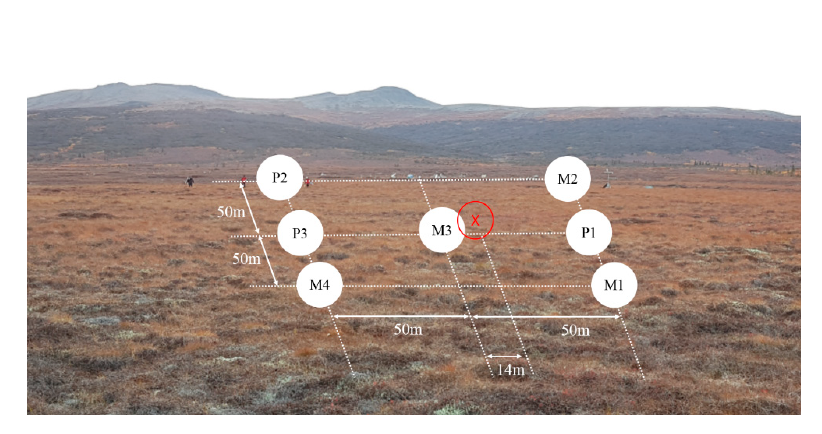
In this study, the air and soil temperatures of the active soil layer were identified from the active development periods in late spring, summer, and early autumn to more realistically describe the dynamic responses of the active layer to temperature changes in Council, west-central Alaska (
Figure 1). During the study period, when the temperature of the upper ground was ≥ 0 °C, the temperatures according to the soil depth were measured at various sampling sites, and air and soil temperatures were analyzed from various perspectives. When the soils freeze the thermal response is very complicated due to latent heat near freezing temperature of 0 °C. In addition, at the environment of the soil temperatures higher than 0 °C is highly associated with heat flux, heat energy productivity, heat productivity from thermal system, thawing of permafrost region, decomposition of microbes and organic matter, and plant growth.
In particular, to predict soil temperatures through the correlation of air and soil temperatures by depth, the model proposed by Park et al. [
21] was modified and employed. The model of Park et al. [
21] predicts the bottom soil temperature using the topsoil temperature.
Thermal response was presented using air temperature, for which sufficient measurement data are available. Further improvement to the results of Park et al. [
21] involved the proposal of a new model for efficiently estimating changes in soil temperatures from the air temperature and soil water content at a depth of 15 cm. The main purpose of this study was to use air temperatures and soil water contents, which are easy to measure, to predict the soil temperature at a shallow depth (15 cm) in an adjacent location. To achieve this goal, three fitting parameters required for predicting soil temperatures using the proposed model were determined and an assessment method that used the soil water content was developed. The accuracy of the proposed temperature model was also evaluated through regression analysis.
3. Results
3.1. Field Measurements of Air and Soil Temperatures and Soil Water Content
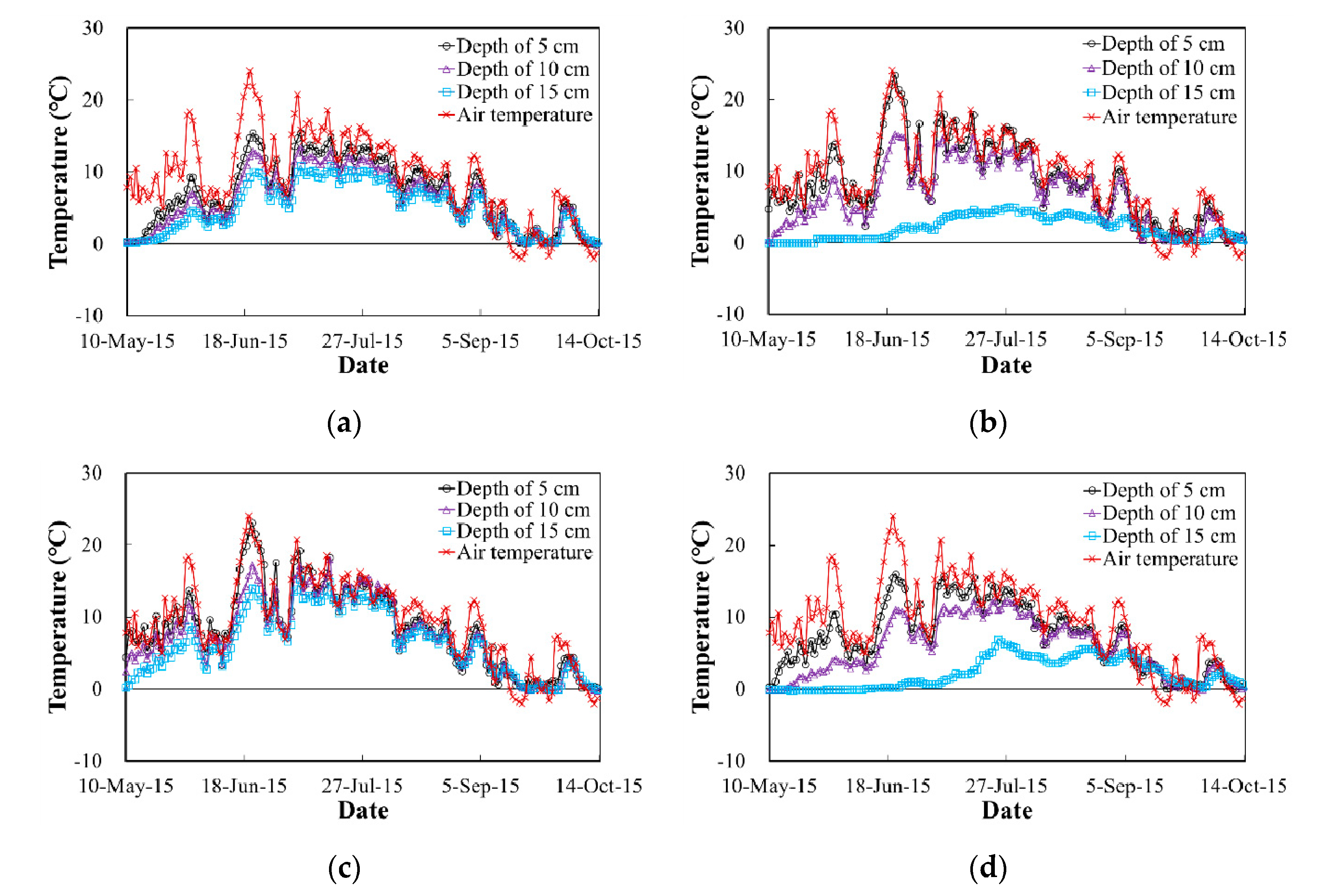
Figure 3 shows the air temperatures continuously measured for 160 days from 10 May to 14 October of 2015 and the soil temperatures measured at locations of M1–M4 during the same period. The air temperature measured at point
x fluctuated from the beginning and reached a maximum value of 24.1 °C around the 42nd day. It continued fluctuating until the 131st day, when it fell below 0 °C, but then fluctuated again until the 157th day, when it once again fell below 0 °C (three days before the end of the study period). During the measurement period, air temperature was generally > 0 °C, except for a few days (days 131–136, 144–145, and 157–160). During the same period, the soil temperatures at depths of 5–15 cm were > 0 °C. This appears to be due to the snow accumulated on the ground surface acting as an effective insulator, thereby causing a difference between the soil and air temperatures [
40,
41].
The air temperature measured at point
x and the soil temperatures measured at locations M1–M4 during the same period showed a tendency to slowly increase at the beginning and then gradually decrease after reaching the maximum values on approximately the 45th day. In
Figure 3, the maximum soil temperature at location M1 is shown to be 15.4 °C. The maximum soil temperatures at locations M2, M3, and M4 were 23.5 °C, 23.1 °C, and 16.0 °C, respectively. These maximum temperatures are indicative of summer in Alaska.
The soil temperatures at locations M1–M4 differed, even at the same depth. This appears to be because of the differences in the soil properties with depth and in the heat transfer of soil. In particular, the amplitude of the daily mean soil temperature changed more drastically as the depth was shallowed when compared to a depth of 15 cm due to the heat from the surface moving toward deeper positions and thus shallower depths were more affected by the heat from the surface. The changes in soil temperatures showed a tendency to decrease as the depth increased, and the maximum soil temperature decreased as the depth increased. Additionally, the soil temperatures of M2 and M4 at a depth of 15 cm showed different patterns of variation, as compared to those of M1 and M3, and temperature changes at other depths (
Figure 3). The reason for this difference may be that there are different thermal properties between the soil and water contents due to spatial heterogeneity in the soil layering and particle size distribution. Moreover, slight time delays between the maximum air temperature and the maximum soil temperature were observed from a depth of 5 cm. According to the observed temperature data during the same period, soil temperature changed from positive to negative values in October and increased to positive values in April–May, even though air temperature had changed significantly.
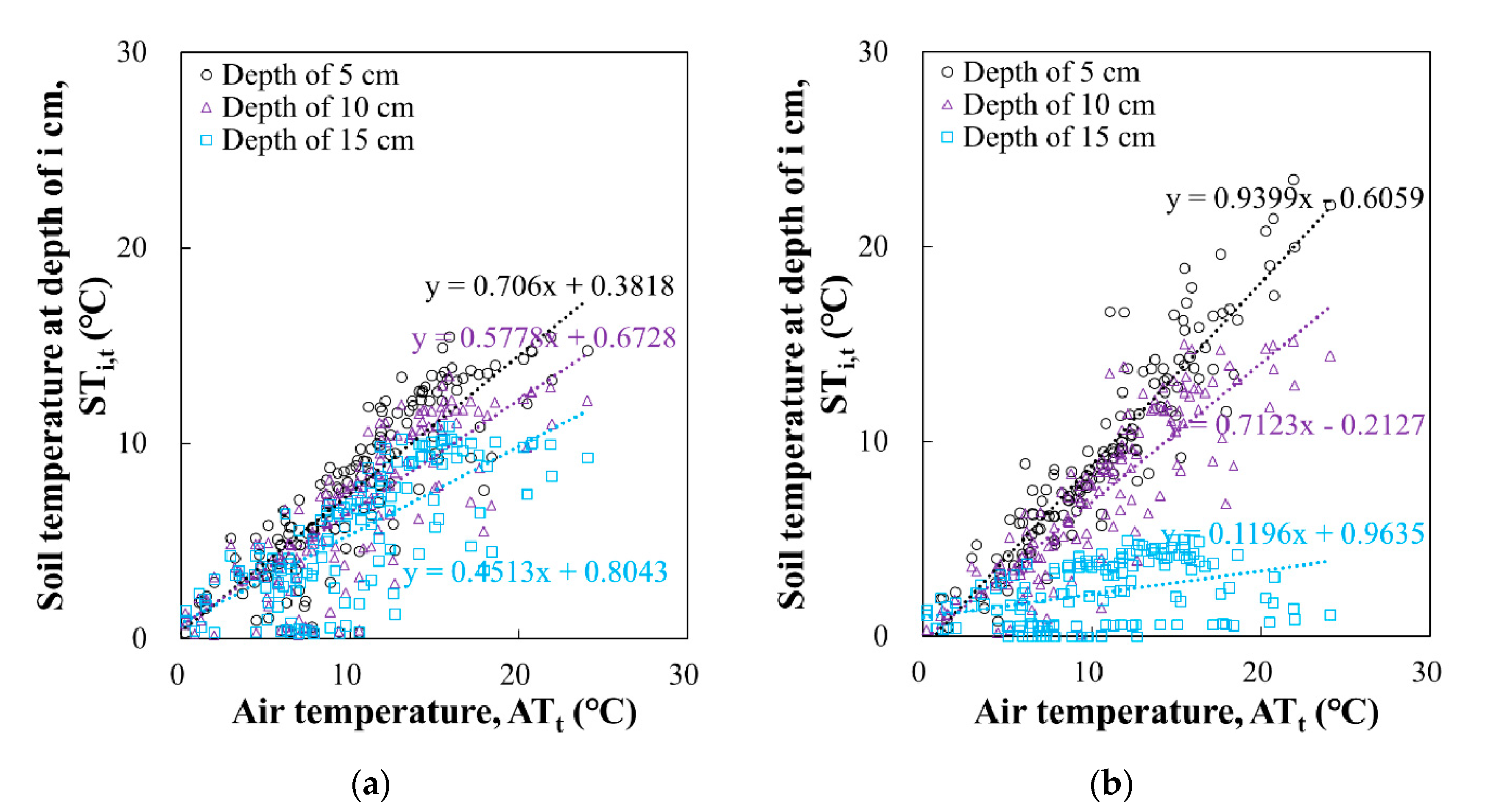
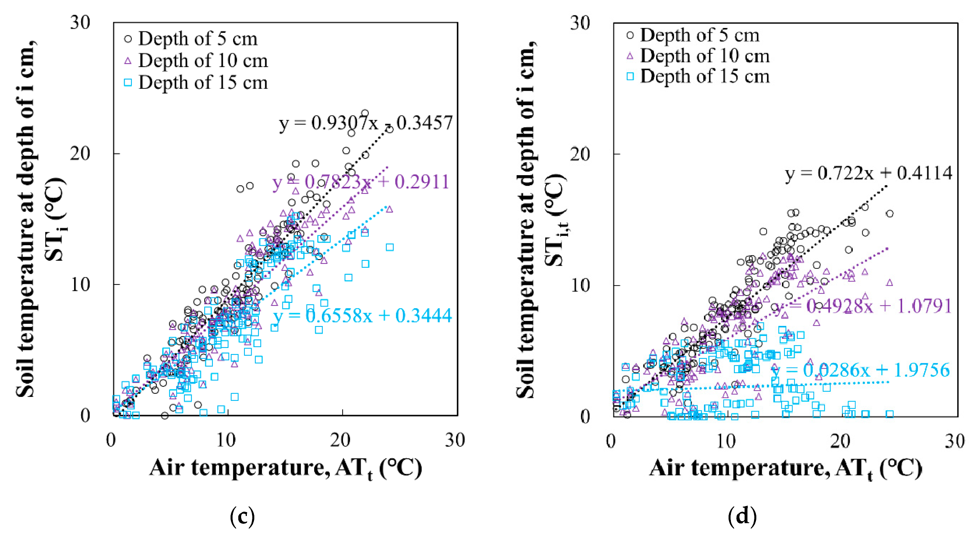
Figure 4 shows the relationships between air temperature (
ATt) and soil temperatures (
STi,t) at depths of 5, 10, and 15 cm; subscripts
i and
t represent the depth from surface and number of days from the start of the study period, respectively. As air temperatures increased, the soil temperatures also showed a tendency to increase. The fitting line equations in
Figure 4 were represented to show of different correlation degrees of soil temperature with air temperature with increasing soil depth. The decrease of gradient of the fitting equation with increasing soil depth in
Figure 4 indicate decrease of correlation between soil temperature and air temperature with increasing depth. The intercept points (soil temperature expected at air temperature of 0 °C) on y axis also increases with increasing soil depth. The fact also implies that soil temperature is less dependent on air temperature for deep depth.
The slopes of the changes in soil temperature for points M2 and M4 at a depth of 15 cm were found to be smaller, when compared to those of M1 and M3 and temperature changes at the same depth (15 cm;
Figure 4). This is because the measured soil temperatures for sites M2 and M4 at a depth of 15 cm were significantly lower, as shown in
Figure 3. Soil acted as a thermal insulator due to the significant differences in the heat transfer characteristics of the soil caused by the different soil properties of locations M2 and M4. The relationship between the two measurements (
ATt and
STi,t) could not be described using a simple mathematical form due to the scattering of the temperature data measured at each point (
Figure 4). This result agrees with the previous findings of Ahmad and Rasul [
42] and Barman et al. [
43].
In
Figure 3 and
Figure 4, the soil temperatures higher > 0 °C with increasing depth were measured based on the active layer development period. Based on the results shown in
Figure 3, the active layer development period was estimated to be between the 1st and 160th days (10 May–14 October in 2015). During this period, a model was developed to predict soil temperatures, which are important for the physical, chemical, and biological processes of terrestrial ecosystems, as noted by Wang et al. [
20] and Park et al. [
21]. To examine changes in soil water contents due to changes in the atmospheric environment, the soil water content was measured over time at a depth of 15 cm (
Figure 5). The soil water content was continuously measured at locations M1–M4 for the same period. The maximum soil water contents at a depth of 15 cm were 23.96% for M1, 11.29% for M2, 37.53% for M3, and 34.81% for M4. At M1, M2, and M3, the soil water content tended to increase and then decrease around the 15th day, increasing again on around the 100th day.
In the case of location M4, the overall soil water content increased until the 23rd day and then remained nearly constant. For location M4, the area was slightly topographically lower in comparison to other locations and thus, rainwater was stored, and snow melted later at this site. This delayed evaporation relative to the other locations, thereby causing the soil water content to be constantly maintained. It appears that the measured soil water contents were also different because the permeability coefficient varied depending on the ground composition, as with soil temperature. However, measurement of field permeability was not possible. This difference in soil water content resulted from the water transmitted to the soil from rain or snow melting on the ground surface. In other words, it occurred because the water content of the ground surface dominated that of the soil. While soil water contents may vary depending upon the flow of groundwater, no groundwater level was detected between the ground surface and a depth of 15 cm at the locations of this study. Therefore, it appears that the soil water content was dominantly affected by rain or snow on the ground surface.
The characteristics of soil particle size distributions and pore sizes among soil particles can be reflected by the standard deviation of the soil water content (wSD). When water is added into soil a medium, it is trapped within the voids (pores) among soil particles. Changes in water content with the moisture or humidity of adjacent environments are highly influenced by the sizes of soil particles and voids. Soils with smaller particles or well-graded soils are more likely to hold water; therefore, the water contents of these soils are less influenced by changes in the environment. Consequently, assessing the variability in water contents, such as the wSD, is important for reflecting temperature changes, considering the relative measures of particle size distributions and sizes of soil pores.
Variability in the soil water contents with time at the sample sites was evaluated and the results are summarized in
Table 2. The mean water contents at the M2 and M4 locations were the lowest and the highest, respectively. The w
SD, which we considered to be the most effective measure for reflecting changes in temperature, was the highest at the M3 location and the lowest at M2.
3.2. Thermal Response Transfer Process
If air temperature is continuously transferred to the ground, temperature changes will occur at shallow depths in the soil. According to Park et al. [
21], temperature changes in a certain area will induce increases in the size of the heat-transferred zone and decrease that of the zone lacking heat transfer. Assuming that the heat transferred by air temperature can be expressed as the cumulative temperature transfer, the thermal response to heat transferred to a soil can be characterized by the cumulative air temperature. Therefore, cumulative air temperature (
CATtr,m), which is the thermal response measured for
m days using Equation (1), can be defined as follows:
where
ATtr,t is the daily mean air temperature and
Tref is the reference temperature (0 °C in this study). Normalized cumulative air temperature,
CAT*
tr,m, is used to express the cumulative air temperature measured in the atmosphere from the start of the measurement period to
m days, as a uniform thermal response can be expressed as:
where
mmax is the number of days (160 days in this study) of the entire measurement period (i.e., the total number of samples for the daily mean temperature). On the basis of the
mth measurement day, the expected future normalized thermal response,
RCST*
tr, m (where RCST represents Reverse Cumulative Soil Temperature), for the rest of the measurement period (
mmax −
m days) can be defined using the
CAT*
tr,m for the measurement period of
m days as:
The relative expression for representing the portion of net heat transfer is denoted as RCAT*tr,m (where RCAT denotes Reverse Cumulative Air Temperature), and indicates the future normalized thermal response. In other words, and RCAT*tr,m of unity (i.e., equal to 1) indicates that the net heat transfer (cumulative air temperature) for the first m days is zero. When RCAT*tr,m = 0, this implies the maximum cumulative air temperature and no additional net heat transfer will occur after the mmax measurement day.
Thermal response was defined in this study based on the air temperature because air temperatures greatly influence soil temperatures. Air temperature has been measured over a long period of time and in various regions. However, there has been relatively little effort made to measure soil temperatures, as the measurement of soil temperature is more difficult than that of air temperature [
33,
34]. It is because and involves considerably higher costs and time investments [
17,
26]. Therefore, a model for predicting soil temperatures uses air temperatures may play an important and effective role in assessing the changes in soil conditions related to global climate change and local disturbances.
3.3. Accumulation of Soil Temperature Characteristics via CAT*tr,m
Abbey et al. [
34] and Dyrness [
44] defined cumulative air temperature to effectively analyze the effects of changes in ground heat flux on the environment. Isaksen et al. [
35], Olivero and Anderson [
45], Ferrant et al. [
46], and Isaksen et al. [
38] further developed cumulative air temperature into a parameter for assessing environmental changes (i.e., thermal responses) using integral-based air temperatures. In this study, the
CSTRCAT15,m (Cumulation of Soil Temperature multiplied by Reverse Cumulative Air Temperature at depth of 15 cm for the first
m days) that was used was based on the sum of thermal responses, which is related to the cumulative air temperature. The
CSTRCAT15,m equation is the sum of the product of the expected normalized thermal response (
RCAT*
tr,m) values until
m days and soil temperatures (
STi,t) at a depth of 15 cm.
In Equation (5), the
CSTRCAT15,m during the entire measurement period (
mmax) can be expressed as
CSTRCAT15,mmax, where
CSTRCAT15,mmax is the maximum cumulative air temperature at depth of 15 cm. Both
RCAT*
tr,t and (
ST15,t−
Tref) for any
mth day were >0 during the testing period.
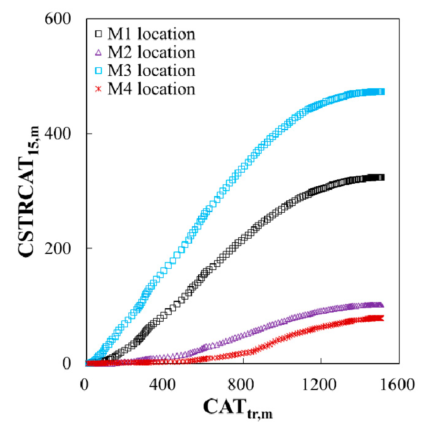
Figure 6 shows the relationship between
CATtr,m and
CSTRCAT15,m by substituting the air temperature measured at point
x and the soil temperatures measured at locations of M1–M4 into Equations (2) and (5). As shown in
Figure 4, the scattered relationship between
ATt and
STi,t was better expressed by implementing the relationship between
CATtr,m and
CSTRCAT15,m.
To normalize the relationship between
CATtr,m and
CSTRCAT15,m shown in
Figure 6,
CSTRCAT15,m was normalized by
CSTRCAT15,mmax at the same depth during the entire measurement period,
mmax, as follows:
where
CSTRCAT*
15,m is the sum of the product of the expected normalized thermal response values measured until
m days, and soil temperature and
CSTRCAT15,mmax is the maximum value of
CSTRCAT15,m at a depth of 15 cm during the entire measurement period,
mmax.
Figure 7 shows the relationship between
CAT*tr,m and
CSTRCAT*15,m for locations M1–M4 obtained using Equations (3) and (6). As shown in the figure, all data rapidly increased at the beginning and gradually converged at a specific point after a slow increase. Moreover, the results shown in
Figure 7 demonstrate that the correlations were improved relative to the
ATt–
STi,t relationship shown in
Figure 4 and the relationship between
CATtr,m and
CSTRCAT15,m shown in
Figure 6. This finding indicates that the quantification of air and soil temperatures using Equations (3) and (6) was more suitable and improved the correlations observed in
Figure 7.
All of the curves shown in
Figure 7 exhibit similar shapes and unique relationships were observed, even though the soil temperatures were measured from different locations. The good fit of the data to these curves indicates that such thermal responses were well expressed by
CAT*tr,m. It appears that the relationship between air and soil temperatures can be theoretically expressed by representing the correlations between
CAT*tr,m and soil temperatures, as shown in
Figure 7. Moreover, it was determined that the cumulative soil temperature was suitable for quantifying heat transfer using thermal responses. In particular, the measured
CSTRCAT*15,m values of M2 and M4 were quite low because the measured temperatures of M2 and M4 were lower than those of M1 and M3 at a depth of 15 cm. Additionally, the prediction curves shown in
Figure 7 accurately reflected the measured temperature differences, confirming that they reasonably represent the changes in temperature and the magnitudes of such changes over time.
The measured soil temperatures at a depth of 15 cm at sites M1 and M3 were lower than those at M2 and M4. The reason for this difference may be that these locations had different soil characteristics (e.g., soil particle size distributions and pore sizes). These soil characteristics were indirectly reflected by the w
SD. It was inferred that the void ratios, defined as the volume of pore spaces over the volume of soil, for sampling sites M2 and M4 were lower than those of M1 and M3; therefore, interactions between the soil water content and air moisture for M2 and M4 were expected to be less than those of M1 and M3. Consequently, the higher soil particle densities of M2 and M4, compared with those of M1 and M3, rendered these sites less dependent on air temperature, which has a lower heat transfer when compared to soils [
47] and more dependent upon underground soil temperatures below a depth of 15 cm.
3.4. Soil Temperature Dynamic Model Using CAT*tr,m
As shown in
Figure 7, a curve representing the relationship between
CSTRCAT*15,m and
CAT*tr,m can be approximated using a simple exponential function, as follows:
where
α and
β are fitting parameters. In Equation (7),
α and
β represent the scale and overall geometry of the relationship between
CSTRCAT*15,m and
CAT*tr,m, respectively. As
CSTRCAT*15,m represents a cumulative value in Equation (7), the actual soil temperature at a certain time point can be obtained by differentiating Equation (7). The mathematical difference between
CSTRCAT*15,m and
CSTRCAT*15,m-1 can be expressed as follows:
By multiplying all of the items in Equation (8) by the denominator (
CSTRCAT15,mmax) of Equation (6), the former may be modified into the product of the expected normalized thermal response and the current temperature, as follows:
Summarizing Equation (9) using Equations (3), (4), (6), and (8) for the current temperature, the soil temperature at a depth of 15 cm on the
mth day can be expressed as:
In this instance, STi,m can be evaluated based on the values of α, β, CSTRCAT15,mmax, and CAT*tr,m.
3.5. Determination of the Fitting Parameters, α and β, for Evaluating CSTRCAT15,mmax
The proposed predictive model for soil temperature using air temperature should account for the wide spatial heterogeneities of different soil properties (e.g., different properties and thermal responses at each location). To represent this, a property that represents the ground is required. The soil water content was selected to improve soil temperature modeling. The process of defining fitting parameters using the wSD was included in this study. Equations (11)–(13) were employed to identify fitting parameters for which the predicted values could be calculated by comparing the wSD measured at a depth of 15 cm with α, β, and CSTRCAT15,mmax.
Table 3 shows the values of
α and
β in Equation (7) at a depth of 15 cm according to the w
SD and
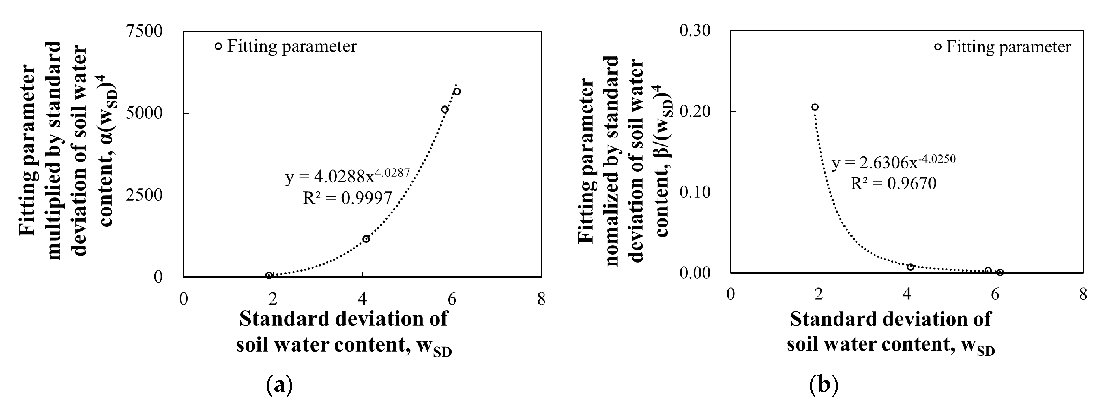
Figure 8 shows the
α and
β values based on
Table 3. Specifically,
Figure 8a,b shows
αw
SD and
β/w
SD. In
Figure 8, w
SD represents the standard deviation of the soil water content for each location. As the Pearson’s correlation coefficients (
R2) of
α and
β for the w
SD were > 0.967,
α and
β can be easily evaluated if only the w
SD is known.
If the least squares method is used, the fitting parameters of
α and
β in Equation (7) can be determined as a function of the w
SD through regression analysis. They can be expressed as follows:
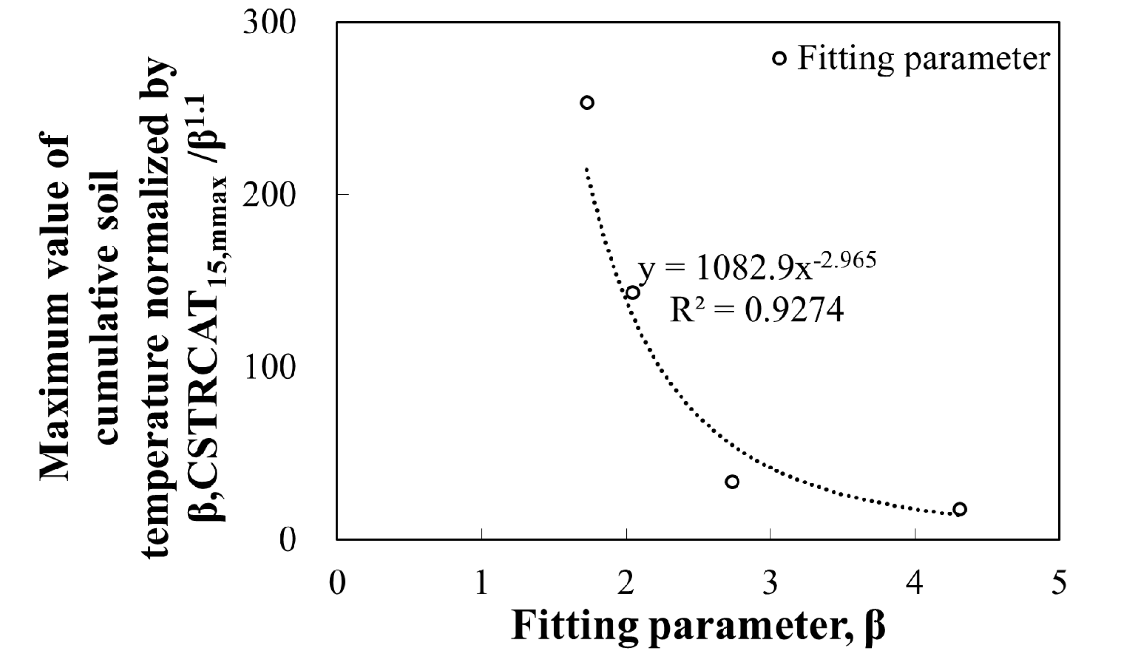
Table 4 and
Figure 9 show the relationship between the maximum cumulative soil temperature normalized by parameter
β (
CSTRCAT15,mmax/β) and
β at a depth of 15 cm. The correlation coefficient between
β and
CSTRCAT15,mmax was 0.9274, indicating that the
CSTRCAT15,mmax value can be easily evaluated if only the value of
β is given. Here, the
CSTRCAT15,mmax value for
β could be expressed as:
The values of α and β only account for when the wSD is within a range of 1.91–6.11, and β is also limited to the range of 1.7266–4.3087. In the case of the fitting parameters of the model, the water content or state variables of the ground must be fully considered. This requires further testing beyond the scope of this study. Here, the spatial heterogeneity of the ground that could not be predicted using air temperature alone was expressed using the soil water content at a depth of 15 cm. It appears that the spatial heterogeneity caused by the differing soil properties measured for each layer can be represented effectively, even if the fitting parameters are acquired by measuring the soil water content at the other depths of 5 cm and 10 cm.
3.6. Summary of Soil Temperature Evaluation
The procedure proposed in this study for evaluating shallow-depth soil temperatures consists of four main steps:
The thermal response of CAT*tr,m is calculated using Equation (3) and mean daily air temperature data;
The expected thermal response, RCAT*tr,m, at the air temperature sampling location during the remaining measurement period is calculated using Equation (4);
The fitting parameters of α and β are determined using Equations (11) and (12), and the maximum cumulative soil temperature, CSTRCAT15,mmax, during the entire measurement period is determined using Equation (13);
Based on the CSTRCAT*15,m and ΔCSTRCAT15,m calculated using Equations (7) and (8), the soil temperature, STi,m–Tref is determined at the depth of interest.
Equation (3) can be used to calculate CAT*tr,m through the air temperature time history. Meanwhile, RCAT*tr,m is obtained once CAT*tr,m is acquired, and CSTRCAT*15,m can be obtained using Equation (7). In this instance, α, β, and CSTRCAT15, mmax are determined using Equations (11)–(13) and the wSD. Finally, the soil temperature, STi,m–Tref, is predicted for the target area.
4. Validation and Discussion
Figure 10 shows the air temperatures measured at location
x (
Figure 2) and the soil water content measured at a depth of 15 cm at locations P1–P3. The additionally obtained w
SD = 6.7723 for P1, w
SD = 8.9907 for P2, and w
SD = 6.4885 for P3. In accordance with the procedure presented in
Section 3.6, the parameters of
α,
β, and
CSTRCAT15, mmax were obtained using the w
SD values obtained from locations P1–P3 (
Table 5). The developed model was implemented using the values shown in
Table 5, and the measured soil temperatures were compared with the predicted
STi,m–
Tref data (
Figure 11).
As shown in
Figure 11, dynamic changes in soil temperatures at a depth of 15 cm over time were effectively predicted. In particular, although the temperatures measured for validation at a depth of 15 cm had different tendencies than those measured for the main investigation at the same depth (
Figure 3), the proposed model exhibited excellent predictive performance for all of the three locations. For location P1, the measured mean and maximum soil temperatures were 2.002 °C and 4.687 °C, while the predicted values were 1.8768 °C and 4.7486 °C, respectively. For location P2, the measured mean and maximum soil temperatures were 5.954 °C and 11.409 °C, while the predicted values were 5.1139 °C and 13.0350 °C. Finally, for location P3, the measured mean and maximum soil temperatures were 2.747 °C and 6.165 °C, while the predicted values were 2.5548 °C and 6.7359 °C.
The difference between the measured and predicted mean soil temperatures was 0.125 °C for P1 and 0.190 °C for P3, while the difference between the measured and predicted maximum soil temperatures was 0.061 °C for P1 and 0.571 °C for P3. These differences in predicted soil temperatures appear to have been caused by the incompleteness of the model. However, the results indicate that it is possible to effectively predict the soil temperatures of all points for depths up to 15 cm at an adjacent location using three simple fitting parameters if air temperature is measured at a location and the wSD of the adjacent location can be measured.
To measure the suitability of the predicted and measured temperature data, the root mean square error (RMSE), mean absolute error (MAE), and
R2 were calculated for the corresponding data. The RMSE is the performance indicator of a regression equation in which the RMSE value increases as the error increases. Mean average error is an indicator of whether there are many or few areas that appear to be outliers [
48].
Table 6 shows the
R2, MAE, and RMSE values of the measured and predicted soil temperatures. As shown, the RMSE value for the data of the proposed model and the measured data ranged from 0.800–2.233, and the MAE ranged from 0.535–1.750. Location P1 exhibited the highest accuracy, as the MAE and RMSE values were 0.535 and 0.743, respectively. The results of P1–P3 exhibited better RMSE and MAE results than those of a previously proposed model [
49].
Figure 12 presents a comparison of the measured and predicted soil temperature data with one-to-one data (blue dotted lines) for each location. Through regression analysis, high
R2 values (0.769–0.809) between the measured and predicted values were obtained. This result is more also more promising than that of another model previously proposed by Abbey et al. [
34] and Hu et al. [
33].
In
Figure 11 and
Figure 12, P1 and P3 exhibited smaller ranges of variation in their maximum temperatures and soil temperatures than P2, as the soil temperatures were less affected by the dynamic changes in the air temperature. This is because the soil temperatures of P1 and P3 were dominantly affected by the soil water content and properties (i.e., thermal conductivity or diffusivity), and thus the uncertainty of soil temperatures [
19] was slightly reduced. Meanwhile, predictions of the soil temperatures at site P2 at a depth of 15 cm exhibited the highest uncertainty, the highest degree of scattering, and the lowest
R2 value. Especially for P2, the predicted temperatures deviated from the measured values in late spring and early summer. During this period, the proposed model underestimated soil temperatures when compared to the measured values (
Figure 11b).
Differences between measured and predicted soil temperatures have also been reported by other researchers (e.g., Romanovsky and Osterkamp [
50,
51]; Jiang et al. [
52]). In general, when the soil water content and air temperature increase, soil temperatures increase due to changes in the soil water content, which plays a larger role than temperature alone. The increase in soil water content increases the thermal conductivity of the soil, thereby directly affecting soil temperatures. In contrast, air temperatures indirectly affect soil temperatures as they change the energy available for heating the soil into soil water content [
52]. Such dynamics may have caused the differences observed between the parameters measured at M1–M4 and those measured at P2 [
33], thereby resulting in underestimated soil temperatures in the late spring and early summer.
As shown in
Figure 11a,c, the initial portions of soil temperatures at a depth of 15 cm for locations P1 and P3 were closed to 0. In regression analyses, data concentrated near a certain value would produce a bias result or a better correlation between measurements and predictions. For the examination of the effect of using concentrated data on a certain value (here, temperatures near 0 °C) on model prediction, the first 40 data points from the start of the temperature measurements at locations P1 and P3 were excluded. The same procedure proposed in this study was implemented. The optimal parameters determined from regression analysis are summarized in
Table 7. Comparison between the prediction and measurement of soil temperatures at a depth of 15 cm with increasing time is represented in
Figure 13. At the beginning of the prediction, the model underestimates the soil temperatures; however, the underestimation trends diminished with increasing time.
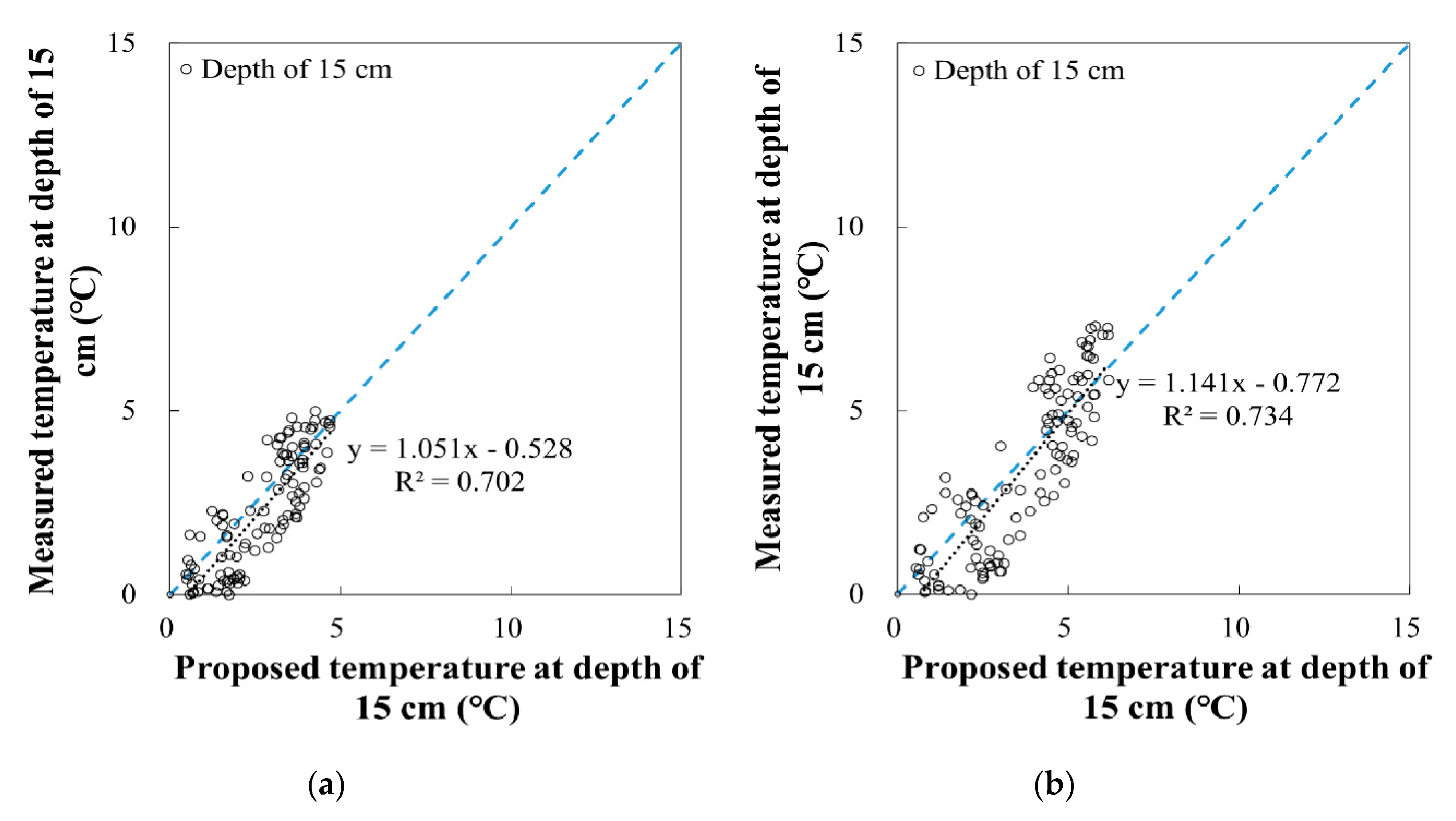
Figure 14 shows point-to-point comparison between predicted and measured soil temperatures at a depth of 15 cm for locations P1 and P3. From the comparison between
R2 values [0.809 in
Figure 12a and 0.804 in
Figure 12c] of the data including the first 40 points and those [0.702 in
Figure 14a and 0.734 in
Figure 14b], the model prediction of the data including the first 40 data points was the better that that excluding the first 40 data points. However, it was concluded that the prediction model implemented in this study reasonably predicts shallow depth soil temperatures based on air temperature and water content.
When developing models, long-term data, such as daily mean temperatures from spring to autumn, are used to reduce the biases of predictions and the variability of temperatures caused by climatic and ground factors, as proposed by Dwyer et al. [
53], and because studies predicting future global soil temperatures have been conducted for spring, summer, autumn, and winter [
24,
54]. Moreover, compared to the models for predicting soil temperatures on a monthly basis [
55,
56], the temperatures predicted on a daily basis are important for studies on sea ice [
57,
58] and crop growth [
35], which are highly temperature-sensitive.
In this study, experimental validation and regression analysis were conducted using long-term data, and important results for the suitability and utility of the proposed soil temperature model were obtained. In northern, high-latitude permafrost regions (e.g., central–northern Alaska), changes in soil temperatures may have serious impacts on the long-term stability of infrastructure, even though they do not present an immediate threat to natural or human systems [
35]. Therefore, the model here can be utilized in various ways and applied to areas where temperatures must be rapidly predicted.
An effective and practical shallow-depth soil temperature model was developed, and its use makes it possible to estimate soil temperatures for adjacent areas and ground layers if the air temperature and w
SD are available for a given location. In previous studies, the measurement of soil temperature has required many parameters [
22,
25], including environmental conditions (e.g., solar radiation, air temperature, and albedo) and soil characteristics (e.g., thermal conductivity, diffusivity, and soil properties), or long analytical periods, such as that used in the Weather Research Forecast model. In contrast, our newly developed model enables rapid analysis with fewer parameters and has a high degree of accuracy for estimating soil temperatures.
Predicting the spatial and temporal patterns of soil temperatures is important because it can promote the understanding of the physical and biological processes of plants, the properties of permafrost and sea ice, and CO
2 and NH
4 emission patterns [
20,
21]. Additionally, the model proposed her is able to determine the most suitable period, work timing, and productivity for field work related to soil heat flux, as well as the heat energy from the geothermal system, biomass, crop flowering time, and appropriate drought monitoring procedures by predicting the soil temperatures of adjacent areas in a rapid and reasonable manner [
59]. As the w
SD is an important factor for determining the model parameters, the application of the w
SD must not be neglected in the estimation of soil temperature.
The developed model has several limitations, despite its simplicity and user-friendliness. Although the mathematical procedure is independent of the measurement locations, at least three standard deviations of soil water content values are required at the target location to determine the three model fitting parameters, α, β, and CSTRCAT15,mmax. This is because these three parameters vary depending upon the temperature changes and soil properties (e.g., thermal conductivity, soil density, and moisture content). Further research is needed to quantify the effects of temperature changes and soil properties on the developed model. Moreover, the continuous measurement of air temperature is required for this model. If air temperature is not measured for a few days, the accuracy of the proposed model will be reduced. Additionally, the model may have prediction errors at shallow depths (depths < 15 cm from the ground surface) due to the spatial variability of soil properties (e.g., soil structure, fabric, or texture). In most cases, it was found that the proposed model can predict soil temperatures for areas where there are differences in soil water contents because it can be assumed that the spatial variability is somewhat uniform at shallow depths. Therefore, it is possible to predict the soil temperatures of areas adjacent to locations at which the air temperature has been measured with some degree of spatial heterogeneity using the soil water content and the measured air temperature.
The proposed model can be used to predict long-term daily mean soil temperature for daily mean air temperature and to evaluate changes in soil temperatures caused by the reactions of spatially heterogeneous (e.g., soil properties and thermal conductivity) soils to the climatic changes expected over a regional scale. The accuracy of the proposed model was improved by including the soil water content, which can reasonably represent soil properties. Therefore, it is expected that the model will be applied to evaluate temperature changes due to soil reactions (soil water content), which require further understanding [
19], as well as to predict daily mean soil temperatures under the influence of climate change, and the resultant changes in soil hydraulic properties (i.e., soil water content).
5. Conclusions
In this study, shallow-depth soil temperatures were measured in Council, Alaska from late spring to early autumn (i.e., the period in which soil temperatures up to a depth of 15 cm exceeded 0 °C). A predictive model of soil temperature for the soil layer located at a depth of 15 cm from the ground surface was developed. This model was developed to predict soil temperatures using air temperatures and soil water contents alone. The proposed model used the concept of thermal responses and the cumulative air temperature. In particular, thermal response (i.e., cumulative air temperature) was used instead of directly using air temperature, so that the soil temperature at a certain depth could be estimated over time in a more consistent and reliable manner.
The mathematical relationship between CSTRCAT*15,m and CAT*tr, m was developed based on the measurement results, and a procedure for predicting soil temperature was proposed. The model was capable of reducing the analytical time needed using only three parameters and yielded accurate prediction results for adjacent locations, even though they had different soil properties. To evaluate the dynamic behavior of soil temperature, the proposed model was validated using soil temperature data obtained from additional locations. When the measured and predicted soil temperatures were compared, it was found that the proposed model accurately predicted soil temperature at a 15 cm depth for various locations. Moreover, soil water content significantly affected soil temperatures. Therefore, the soil water content must not be neglected in the estimation of soil temperatures because the wSD is an important factor for determining the parameters of the proposed model.
The model developed in this study can contribute to the fast and accurate measurement of soil temperatures in the active soils layer of permafrost at various locations, and can provide useful information for studies related to spatial changes in soil environments. It will also be helpful for determining the most suitable periods, work timing, and productivity for field work when planning crop flowering times and drought monitoring. However, further research is needed to generate additional spatiotemporal information related to the variability of soil temperatures over large geographic areas.

