Range Localization of a Moving Source Based on Synthetic Aperture Beamforming Using a Single Hydrophone in Shallow Water

Abstract

To localize a moving source in shallow water with a single hydrophone, a passive range localization method based on synthetic aperture beamforming is proposed. First, the horizontal wavenumber spectrum excited by the source is obtained by synthetic aperture beamforming. Then, according to the theoretical derivation (when the integration time is short, the maximum value of the horizontal wavenumber spectrum is related to the average horizontal wavenumber and the radial velocity of the source), the radial velocity can be obtained after obtaining the average horizontal wavenumber. Finally, in the case where there is a closest point of approach (CPA), the range can be recovered from estimation of the range and time of CPA, and from the constant source speed alone the linear track by fitting the source velocity with the model of radial velocity. The only a priori information required is the sound velocity in water. The processing results using simulated data and SWellEx-96 experimental data show that the proposed method can effectively estimate the range of a moving source in shallow sea.

1. Introduction

Acoustic methods for localizing a source in an underwater acoustic waveguide, including direction finding and range and depth estimation, are a topic of great interest in the field of underwater acoustic signal processing. Popular methods for estimating the source range and depth are matched field processing (MFP) [1,2] and matched mode processing (MMP) [3,4], which require multiple hydrophones to form a vertical or horizontal array to receive the source radiated noise. Knowledge of the environment, such as the sound speed profile (SSP) and the geoacoustic parameters, is also needed to calculate the copy field vector for MFP or the modal coefficient vector for MMP using a propagation model to estimate source range and depth. The MFP and MMP methods are often plagued by environmental mismatch problems: if the assumed environment differs from the true environment, there may be large error in the final position estimate [5,6]. A number of robust localization algorithms have been developed to solve the mismatch problem [7,8,9,10], and will not be described here.

In actual use, the hydrophone array is expensive, and it is cumbersome to deploy at sea. Therefore, the idea of using a single hydrophone to perform source range localization emerged. A single hydrophone can be deployed more quickly and flexibly, at a lower cost, and monitoring of a large area can be realized by mass deployment. The principle of the early single-hydrophone localization methods is similar to the MFP method [11,12]. In general, a wideband acoustic signal or a pulsed acoustic signal is required, as well as accurate environmental information, so there is still the problem of environmental mismatch. Later, methods based on the inherent characteristics of the sound field were developed. Cockrell and Schmidt [13] developed a ranging method based on the waveguide invariant. This method calculates the slope of interference patterns in different regions on the range–frequency plane and uses the principle of waveguide invariance to achieve robust range measurement. Rakotonarivo and Kuperman [14] pointed out that the magnitude of the square of the difference between the acoustic field at two different ranges contains information about the range interval, and the range rate can be ascertained. Bonnel et al. [15] developed a single-hydrophone ranging method using the nonlinear signal processing method warping transform to filter the modes. Once modal arrivals have been separated, the source range can be estimated using the conventional modal dispersion technique. Kuznetsov et al. [16] have also developed a single-hydrophone ranging method based on repeat Fourier transformation of the interference pattern formed during source motion.

Here we derive a source range localization method based on single-hydrophone synthetic aperture beamforming. The horizontal wavenumber spectrum excited by the source can be obtained by the synthetic aperture beamforming of a single hydrophone. According to the relationship between the maximum value of the horizontal wavenumber spectrum, the average horizontal wavenumber, and the radial velocity of the source, range localization can be achieved.

The method is derived and illustrated with simulated results in Section 2 and Section 3, respectively. Then, the method is validated with data from a shallow water experiment in Section 4. Section 5 concludes the work.

2. The Range Localization Method

We consider a range-independent shallow ocean environment and a moving source with a depth z_s and constant speed v₀ during the observation time T. The radial velocity is given by

$$\begin{array}{cc}\hfill v_s\left(t\right)& =\frac{\delta r}{\delta t}\left(t\right)\hfill \\ & =\left|\frac{\sqrt{r_0^2+{\left(t-t_0\right)}^2{v}_0^2}-\sqrt{r_0^2+{\left(t-t_0-\delta t\right)}^2{v}_0^2}}{\delta t}\right|\hfill \end{array},$$

(1)

where $r_0$ and $t_0$ are the range at the closest point of approach (CPA) and the time of CPA, respectively, and $\delta t$ is the variation of time associated to $\delta r$, the radial range variation for each acquisition time $t$.

The normal mode theory expression of the pressure field received at a receiver at a depth z_r and time $t$ is

$$p\left(t\right)={\displaystyle \sum }_{m=1}^M\sqrt{\frac{2\pi }{k_m{r}_t}}{\varphi }_m\left(z_s\right){\varphi }_m\left(z_r\right)e^{-i{k}_m{r}_t-{\alpha }_m{r}_t-i\pi /4},$$

(2)

where $r_t$ is the source range at time $t$, ϕ_m(z) is the $m$th mode depth function, k_m is the $m$th horizontal wavenumber, and α_m is the $m$th mode attenuation coefficient. $M$ is the number of modes that can be propagated in the current environment.

The pressure field at different times is beamformed as follows [17,18]:

$$g(k_r)=\frac{e^{i\pi /4}}{\sqrt{2\pi k_r}}{\displaystyle {\int }_{t_1}^{t_2}p\left(t\right)e^{i{k}_{r}t}\sqrt{r_t}dt},$$

(3)

where $t_1$ and $t_2$ represent the start and end moments of the observation time $T$, respectively, and $e^{i{k}_{r}t}$ is the steering vector and $k_r$ is a variable.

In [17] the observation time $T$ should set to be long enough to separate different horizontal wavenumbers of modes. Here, we set the observation time in the opposite way. When the observation time $T$ is short, the radial velocity can be considered to be constant, which is represented by ${\overline{v}}_s$. Within the observation time $T$, the source range $r_t$ can be expressed as

$$r_t=r_{t_1}+{\overline{v}}_{s}t,$$

(4)

where $r_{t_1}$ represents the range at time $t_1$. After substituting the normal mode expression into Equation (3), one obtains

$$\begin{array}{cc}\hfill g\left(k_r\right)& \simeq {\displaystyle \sum _{m=1}^M\frac{{\varphi }_m\left(z_s\right){\varphi }_m\left(z_r\right)}{\sqrt{k_r{k}_m}}{\displaystyle {\int }_{t_1}^{t_2}{e}^{i{k}_{r}t-i{k}_m{r}_t-{\alpha }_m{r}_t}dt}}\hfill \\ & ={\displaystyle \sum _{m=1}^M{a}_m\frac{{\varphi }_m\left(z_s\right){\varphi }_m\left(z_r\right)}{k_r-k_m{\overline{v}}_s+i{\alpha }_m{\overline{v}}_s}}\hfill \\ & ={\displaystyle \sum _{m=1}^M{a}_m\frac{{\varphi }_m\left(z_s\right){\varphi }_m\left(z_r\right)}{k_r-\left(\overline{k}+\delta k_m\right){\overline{v}}_s+i{\alpha }_m{\overline{v}}_s}}\hfill \end{array},$$

(5)

where

$$a_m=\frac{e^{i{k}_r{t}_2-i{k}_m{v}_s{t}_2-{\alpha }_m{v}_s{t}_2}-e^{i{k}_r{t}_1-i{k}_m{v}_s{t}_1-{\alpha }_m{v}_s{t}_1}}{i\sqrt{k_r{k}_m}}{e}^{-i{k}_m{r}_{t_1}-{\alpha }_m{r}_{t_1}},$$

and the wavenumbers can be expressed as $k_m=\overline{k}+\delta k_m$, where $\overline{k}$ is the average horizontal wavenumber of the modes since $\delta k_m\ll \overline{k}$ (typically, $\delta k_m/\overline{k}\sim \mathcal{O}({10}^{-2})$ for discrete mode wavenumbers, which are between $k_{\min }=\omega /c_b$ and $k_{\max }=\omega /\min (c_w)$ where $c_b$ and $c_w$ are the sound speeds at the bottom surface and in the water, respectively [14]. For some lower frequencies’ cases, $\delta k_m/\overline{k}\sim {10}^{-1}$). Then $g\left(k_r\right)$ can be written as

$$g\left(k_r\right)\simeq {\displaystyle \sum _{m=1}^M\frac{a_m{\varphi }_m\left(z_s\right){\varphi }_m\left(z_r\right)}{k_r-\overline{k}{\overline{v}}_s+i{\alpha }_m{\overline{v}}_s}}.$$

(6)

It can be seen from Equation (6) that the horizontal wavenumber spectrum $g\left(k_r\right)$ will have maxima for $k_r=\overline{k}{\overline{v}}_s$, noting that the mode attenuation coefficient is generally orders of magnitude smaller than the horizontal wavenumber. The average phase speed ${\overline{v}}_p$ can be approximated by the sound speed in water: ${\overline{v}}_p\approx c_w$, and we can easily obtain the average horizontal wavenumber since we have that $\overline{k}\left(f\right)=2\pi f/{\overline{v}}_p$ for a particular frequency (narrowband case). Furthermore, the average radial velocity within the observation time $T$ can be obtained as

$${\overline{v}}_s=\frac{k_r}{\overline{k}}.$$

(7)

In the calculation process, the term $\sqrt{r_t}$ in Equation (3) can be considered to be constant within a short observation period $T$, and thus can be set to 1 without affecting the subsequent results. Further, Equation (3) can be conveniently calculated using a method such as fast Fourier transform (FFT).

After obtaining the radial velocity, we can easily obtain the source speed $v_0$, the range and time of CPA, $r_0$ and $t_0$, according to Equation (1) using the least squares criterion and then calculate the source range as follows

$$r_t=\sqrt{r_0^2+{\left(t-t_0\right)}^2{v}_0^2}.$$

(8)

For a broadband case, the frequency processing gain can be obtained in a manner of sub-band division and non-coherent accumulation. Assume that the number of sub-bands divided is $L$, and the center frequency corresponding to each sub-band is $f_l$, where $l=1,2,\cdots ,L$. Each sub-band is processed according to Equation (3) to obtain the sub-band horizontal wavenumber spectrum $g{\left(k_r\right)}_{f_l}$, where $l=1,2,\cdots ,L$. Since the average horizontal wavenumbers corresponding to different frequencies are different, the peak positions of the sub-band horizontal wavenumber spectrums are also different. Therefore, the sub-band horizontal wavenumber spectrum cannot be directly added together. Here, we choose any one of the sub-band center frequencies as the reference frequency $f_{\mathrm{ref}}$, and convert the horizontal wavenumber spectrum of each sub-band into a form relative to the reference frequency by stretching/compression transformation ($g{\left(k_r\right)}_{f_l}\Rightarrow g{\left(k_r\left(f_l/f_{\mathrm{ref}}\right)\right)}_{f_l}$). Finally, we can obtain the following broadband horizontal wavenumber spectrum

$$G\left(k_{r,\mathrm{ref}}\right)={\displaystyle \sum }_{l=1}^L{\left|g{\left(k_{r,\mathrm{ref}}\frac{f_l}{f_{\mathrm{ref}}}\right)}_{f_l}\right|}^2,$$

(9)

where $k_{r,\mathrm{ref}}$ is the variable corresponding to the reference frequency $f_{\mathrm{ref}}$. The broadband horizontal wavenumber spectrum is similar to the narrowband horizontal wavenumber spectrum at a frequency $f_{\mathrm{ref}}$, so that the average radial velocity can be estimated as shown in Equation (10), similarly to the process of obtaining Equation (7)

$${\overline{v}}_s=\frac{k_{r,\mathrm{ref}}}{{\overline{k}}_{\mathrm{ref}}},$$

(10)

where the average horizontal wavenumber ${\overline{k}}_{\mathrm{ref}}=2\pi f_{\mathrm{ref}}/{\overline{v}}_p$.

It can be seen from Equation (7) that the approximation of the average horizontal wavenumber by the wavenumber in water causes a bias on the estimation of the average radial velocity, which will in turn affect the accuracy of the range estimation. Assuming that the error of the average horizontal wavenumber is $\delta k$, then the estimation error of the average radial velocity is given here [14]

$$\begin{array}{cc}\hfill \Delta {\overline{v}}_s& ={\overline{v}}_s-{{\overline{v}}_s|}_{\mathrm{error}}=\frac{k_r}{\overline{k}}-\frac{k_r}{\overline{k}+\delta k}\hfill \\ & ={\overline{v}}_s\frac{\delta k/\overline{k}}{1+\delta k/\overline{k}}\hfill & \end{array},$$

(11)

and the maximum error of the horizontal wavenumber is $\delta k=k_{\max }-k_{\min }$. According to the previous description, $\delta k/\overline{k}$ is small since $\delta k\ll \overline{k}$, so the radial velocity estimation error is also small, ensuring the accuracy of the range localization.

So far, we have completed the theoretical derivation of the source range localization. The effectiveness of the method will be verified using simulation and at-sea data in the next two sections.

3. Simulation and Results

We consider an 88 m depth waveguide with a negative gradient SSP as shown in Figure 1. It consists of a 10 m isothermal mixed layer with a sound speed of 1533 m/s. The sound speed reduces linearly to 1478 m/s at a depth of 40 m and then remains unchanged until the bottom at 88 m. The bottom sound speed is 1650 m/s, the bottom density is 1.76 g/cm³, and the bottom attenuation is 0.8 $\mathrm{dB}/\mathsf{\lambda }$. We assume that the source speed is $v_0=2.0 \mathrm{m}/\mathrm{s}$, the range of CPA is $r_0=1000 \mathrm{m}$, the time of CPA is $t_0=1000 \mathrm{s}$, the source depth is 50 m, a narrowband signal of 350 Hz is emitted, and the depth of the receiver is 70 m.

The received sound pressure is calculated using the Kraken normal mode model [19]. The relationship between the real part of the sound pressure and time is shown in Figure 2a. After zooming in to reveal the details, it can be seen from Figure 2b that the real part of the sound pressure exhibits obvious periodicity. According to the above theoretical derivation, this period is related to the average horizontal wavenumber and the radial velocity.

In the simulation, the observation period is set to be $T=0.5\mathrm{s}$, and Equation (3) is calculated using the 128-point FFT. The horizontal wavenumber spectrum of the first-time step is obtained and shown in Figure 3. It can be seen that the maximum value of the spectrum appears at $k_r=2.651$. We set the average phase velocity to be ${\overline{v}}_p=1478\mathrm{m}/\mathrm{s}$ and obtain $\overline{k}=1.4879{\mathrm{m}}^{-1}$. Then an estimated value of the radial velocity ${\overline{v}}_s=1.7817\mathrm{m}/\mathrm{s}$ can be obtained according to Equation (7). Following this method, the radial velocity in the observation time of 6000 seconds is obtained as shown in Figure 4, from which we can see that the estimated radial velocity remains consistent with its theoretical value (the black solid line in the figure). After calculating the source speed $v_0$, and the range and time of CPA, $r_0$ and $t_0$, using Equation (1), we can obtain the source range estimation using Equation (8). The result is shown in Figure 5.

It can be seen from the above analysis that the range localization result obtained by the simulation data is good. The processing result of the SWellEx-96 experimental data is given below.

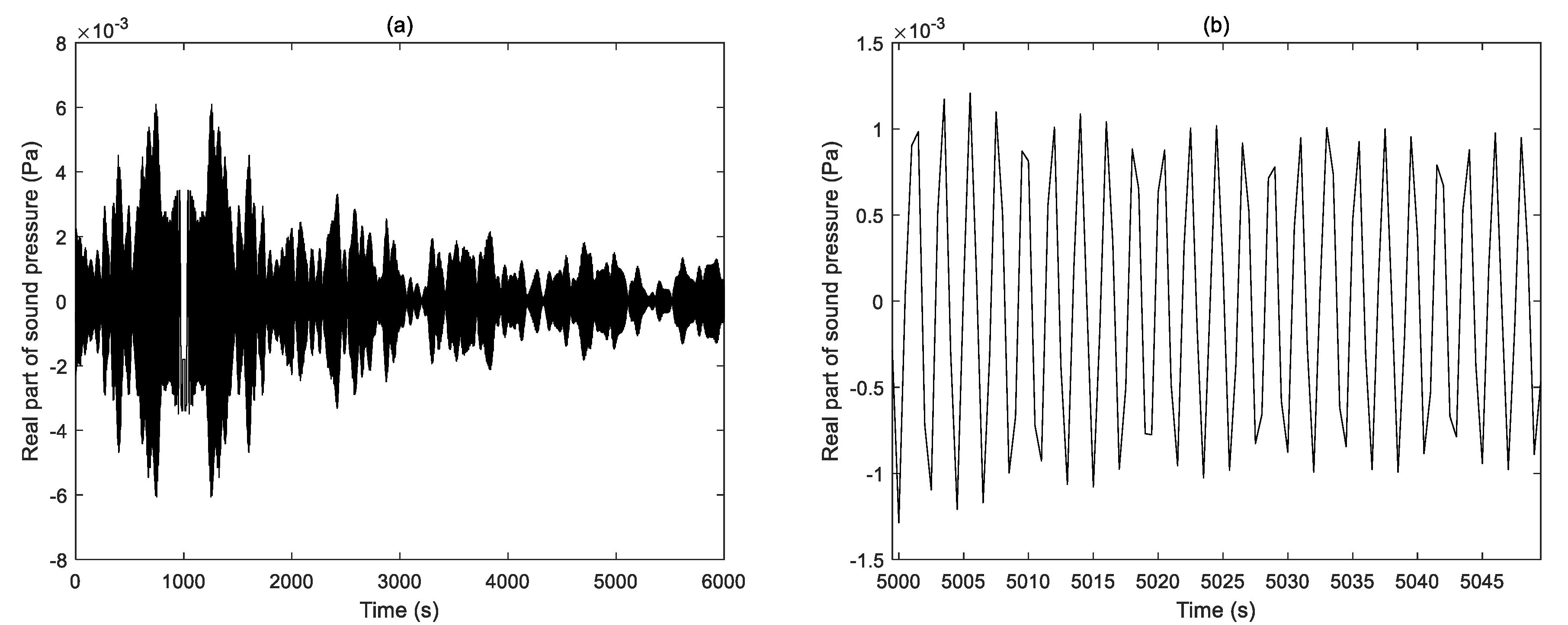
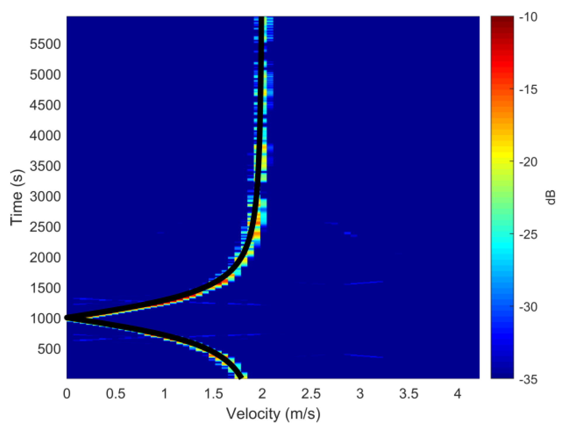
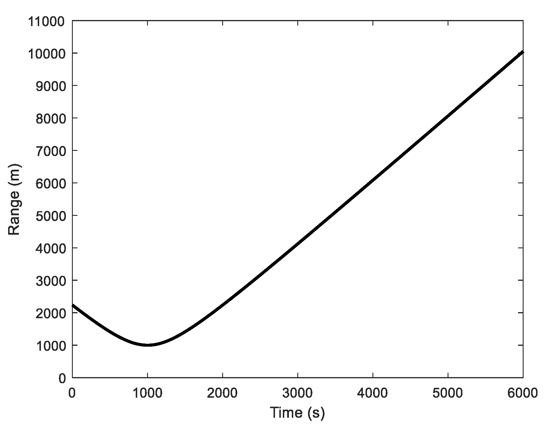
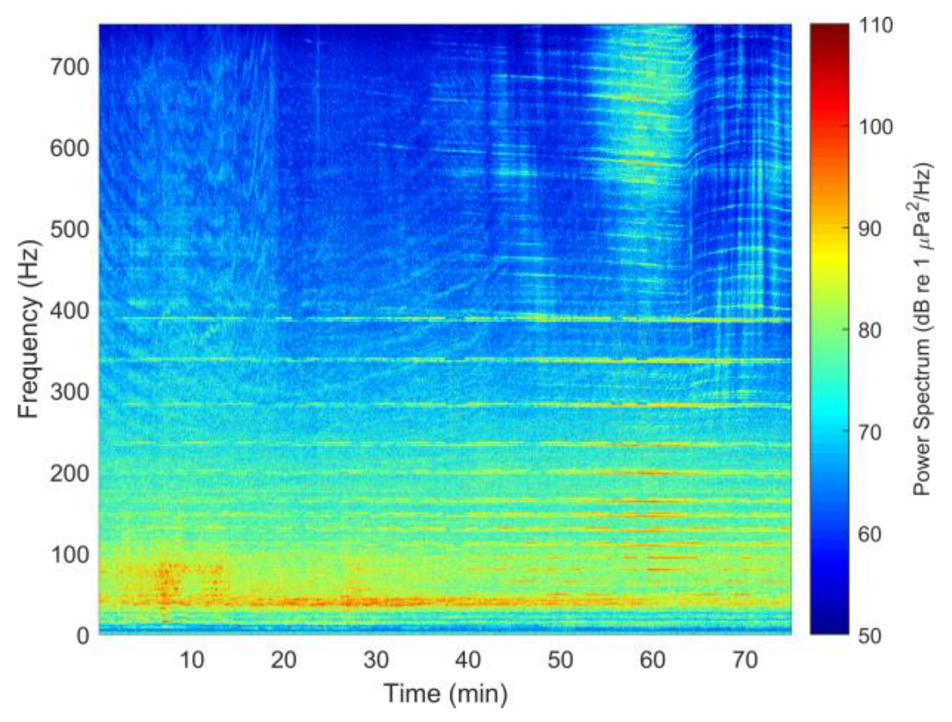
4. SWellEx-96 Experimental Data Analysis

4.1. Experiment Description

Data from the SWellEx-96 experiment were used. The SWellEx-96 experiment was conducted by the Marine Physical Lab in the littoral waters just outside the port of San Diego in May 1996. The environmental information and data are available online [20]. Therefore, they are widely used to verify the performance of underwater target detection [21], localization [22], tracking [23], and underwater acoustic inversion [24] methods.

The receiving arrays used in the experiment include a vertical line array (VLA), a tilt line array (TLA), and two horizontal line arrays (HLA). The experiment is divided into two events: S5 and S59. Sound sources in both events travel along the contour line and are suitable for signal processing in a range-independent sound field environment, and event S59 has one more interference source than event S5. Here, the data of the vertical array from event S5 are used to verify the performance of the proposed range localization method.

Figure 6 shows the ship trajectory for event S5, with two sources being towed at depths of 54 m and 9 m, respectively. The deeper source emits comb-like single-frequency signals at various signal-to-noise ratios (SNR) and frequencies from 49 to 400 Hz, and the shallower source emits 9 single-frequency signals with a frequency range of 109 to 385 Hz. The sampling rate is 1500 Hz. The SSP was measured using a CTD several times during the 75 min duration of the experiment.

The environmental parameters of the waveguide and the configuration of the VLA are shown in Figure 7. The depth of the highest array element is 94.125 m and the depth of the lowest one is 212.25 m.

4.2. Data Processing Results and Analysis

In the following, the source range is estimated from the analysis of the signal received at the deepest array sensor. The results given below are similar when processing the signal measured at the other array elements. As shown in Figure 8, the time–frequency diagram of the measured signal shows that there is a suspected strong interference in the frequency band below 100 Hz around the 10th minute, which will have an impact on the radial velocity estimation based on single-frequency signal processing. Around the 60th minute, there are strong interference patterns in the ~500 to 700 Hz frequency band, which is caused by the noise radiated by the source ship.

4.2.1. Narrowband Source Range Localization

For the narrowband case, $p\left(t\right)$ in Equation (2) is calculated and the 127 Hz line is extracted from the spectrogram of the time series that was acquired continuously during the 75 min of the experiment, which is shown in Figure 9. The size of the window for the FFT is 1 s and the number of FFT points is 1500.

The time step is set to be $T=1\mathrm{s}$, and Equation (3) is calculated using the 128-point FFT. The horizontal wavenumber spectrum of the first-time step is obtained and shown in Figure 10. The maximum value of the spectrum appears at $k_r=1.325$. We set the average phase velocity to be ${\overline{v}}_p=1490\mathrm{m}/\mathrm{s}$ and obtain $\overline{k}=0.5355{\mathrm{m}}^{-1}$. Then an estimated value of the radial velocity ${\overline{v}}_s=2.4741\mathrm{m}/\mathrm{s}$ can be obtained according to Equation (7). Following this method, the radial velocity in the 75 min duration of the experiment is obtained as shown in Figure 11, wherein the black solid line is the maximum point. It can be seen that the estimation of the radial velocity is good for most of the time. Around the 10th minute, some points with large deviations appear, caused by the strong interference mentioned above.

The best fit between the model of radial velocity given in Equation (1) and the estimated source velocity can be obtained using the least squares criterion, as shown in Figure 12. This provides a range and time of CPA of $r_0=1058\mathrm{m}$ and $t_0=3520\mathrm{s}$, respectively, and a linear source velocity along the track of $v_0=2.48\mathrm{m}/\mathrm{s}$. These estimated values are in good agreement with the GPS data, for which the range and time of CPA are $r_{0,\mathrm{GPS}}=902\mathrm{m}$ and $t_{0,\mathrm{GPS}}=3540\mathrm{s}$, respectively, and the linear source velocity is $v_{0,\mathrm{GPS}}=2.55\mathrm{m}/\mathrm{s}$. This also indicates that the outliers of the radial velocity estimate have little impact on the final range parameter estimates.

The source range is estimated and shown in Figure 13. It can be seen that the estimated source ranges are in good agreement with the ranges from GPS data, and exhibit a bias of 6.23%.

4.2.2. The Broadband Case

In the experiment, the sound source emits signals of multiple frequencies, so the broadband range localization method can also be used to estimate the source range. Three frequencies of 109, 127, and 130 Hz are selected to estimate the source range, and the remaining parameter settings are the same as the narrowband case. According to the calculation of Equation (9), the radial velocity estimation result is obtained and shown in Figure 14. It can be seen from the figure that the interference in the 10th minute has no effect on the radial velocity estimation result, showing the advantage of broadband processing. After obtaining the radial velocity using the broadband method, the source range estimation can be accomplished following the same steps as the narrowband case, which will not be described herein again.

5. Conclusions

In this paper, the estimation of the source radial velocity is realized based on the synthetic aperture beamforming method. Then, the least squares criterion is used to estimate the range and time of CPA and the source velocity. Finally, source range localization is accomplished. The proposed method is validated to be effective by both simulation data and SWellEx-96 experimental data. This paper presents a method for estimating the radial velocity in both narrowband and broadband forms. The broadband form is more stable in the presence of interference in the environment or low SNR case. Because the FFT algorithm is used in the calculation of the horizontal wavenumber spectrum, the running speed of the method can be increased and a shorter running time can be obtained. Since only the sound speed in water is needed as a priori information, the proposed method is robust to the environmental uncertainty. It should be noted that for the case of no CPA present, after the radial velocity is obtained, the estimation of the source range can still be realized based on the waveguide invariant method. In this case, some broadband signal information is needed, and the specific process can be found in [14].

References

1. Bucker, H.P. Use of calculated sound fields and matched-field detection to locate sound sources in shallow water. J. Acoust. Soc. Am. 1976, 59, 368–373. [Google Scholar] [CrossRef]
2. Baggeroer, A.B.; Kuperman, W.A.; Mikhalevsky, P.N. An overview of matched field methods in ocean acoustics. IEEE J. Ocean. Eng. 1993, 18, 401–424. [Google Scholar] [CrossRef]
3. Shang, E.C.; Clay, C.S.; Wang, Y.Y. Passive harmonic source ranging in waveguides by using mode filter. J. Acoust. Soc. Am. 1985, 78, 172–175. [Google Scholar] [CrossRef]
4. Yang, T.C. A method of range and depth estimation by modal decomposition. J. Acoust. Soc. Am. 1987, 82, 1736–1745. [Google Scholar] [CrossRef]
5. Balzo, D.R.D.; Feuillade, C.; Rowe, M.M. Effects of water-depth mismatch on matched-field localization in shallow water. J. Acoust. Soc. Am. 1988, 83, 2180–2185. [Google Scholar] [CrossRef]
6. Tolstoy, A. Sensitivity of matched field processing to sound-speed profile mismatch for vertical arrays in a deep water Pacific environment. J. Acoust. Soc. Am. 1989, 85, 2394–2404. [Google Scholar] [CrossRef]
7. Yang, K.; Ma, Y.; Zhang, Z.; Zou, S. Robust adaptive matched field processing with environmental uncertainty. Acta Acust. 2006, 31, 255–262. [Google Scholar]
8. Debever, C.; Kuperman, W.A. Robust matched-field processing using a coherent broadband white noise constraint processor. J. Acoust. Soc. Am. 2007, 122, 1979–1986. [Google Scholar] [CrossRef]
9. Liu, Z.-W.; Sun, C.; Xiang, L.-F.; Yi, F. Robust source localization based on mode subspace reconstruction in uncertain shallow ocean environment. Acta Phys. Sin. 2014, 63, 034304. [Google Scholar]
10. Yang, T.C. Data-based matched-mode source localization for a moving source. J. Acoust. Soc. Am. 2014, 135, 1218–1230. [Google Scholar] [CrossRef]
11. Frazer, L.N.; Pecholcs, P.I. Single-hydrophone localization. J. Acoust. Soc. Am. 1990, 88, 995–1002. [Google Scholar] [CrossRef]
12. Jesus, S.M.; Porter, M.B.; Stephan, Y.; Demoulin, X.; Rodriguez, O.C.; Coelho, E.M.M.F. Single hydrophone source localization. IEEE J. Ocean. Eng. 2000, 25, 337–346. [Google Scholar] [CrossRef]
13. Cockrell, K.L.; Schmidt, H. Robust passive range estimation using the waveguide invariant. J. Acoust. Soc. Am. 2010, 127, 2780–2789. [Google Scholar] [CrossRef] [PubMed]
14. Rakotonarivo, S.T.; Kuperman, W.A. Model-independent range localization of a moving source in shallow water. J. Acoust. Soc. Am. 2012, 132, 2218–2223. [Google Scholar] [CrossRef] [Green Version]
15. Bonnel, J.; Thode, A.M.; Blackwell, S.B.; Kim, K.; Macrander, A.M. Range estimation of bowhead whale (Balaena mysticetus) calls in the Arctic using a single hydrophone. J. Acoust. Soc. Am. 2014, 136, 145–155. [Google Scholar] [CrossRef]
16. Kuznetsov, G.; Kuz’kin, V.; Pereselkov, S. Spectrogram and localization of a sound source in shallow water. Acoust. Phys. 2017, 63, 449–461. [Google Scholar] [CrossRef]
17. Yang, T.C. Source depth estimation based on synthetic aperture beamfoming for a moving source. J. Acoust. Soc. Am. 2015, 138, 1678–1686. [Google Scholar] [CrossRef]
18. Frisk, G.V.; Lynch, J.F.; Rajan, S.D. Determination of compressional wave speed profiles using modal inverse techniques in a range-dependent environment in Nantucket Sound. J. Acoust. Soc. Am. 1989, 86, 1928–1939. [Google Scholar] [CrossRef]
19. Duncan, A. Underwater Acoustic Propagation Modelling Software. Available online: https://cmst.curtin.edu.au/products/underwater/ (accessed on 17 December 2019).
20. MPL. The SWellEx-96 Experiment. Available online: http://www.mpl.ucsd.edu/swellex96/index.htm (accessed on 10 October 2019).
21. Sha, L.; Nolte, L.W. Bayesian sonar detection performance prediction with source position uncertainty using SWellEx-96 vertical array data. IEEE J. Ocean. Eng. 2006, 31, 345–355. [Google Scholar] [CrossRef]
22. Michalopoulou, Z.-H. Matched-impulse-response processing for shallow-water localization and geoacoustic inversion. J. Acoust. Soc. Am. 2000, 108, 2082–2090. [Google Scholar] [CrossRef]
23. Yardim, C.; Gerstoft, P.; Hodgkiss, W.S. Geoacoustic and source tracking using particle filtering: Experimental results. J. Acoust. Soc. Am. 2010, 128, 75–87. [Google Scholar] [CrossRef] [PubMed] [Green Version]
24. Musil, M.; Chapman, N.R.; Wilmut, M.J. Range-dependent matched-field inversion of SWellEX-96 data using the downhill simplex algorithm. J. Acoust. Soc. Am. 1999, 106, 3270–3281. [Google Scholar] [CrossRef]
Figure 1. Typical shallow-ocean sound field environment for simulation.
Applsci 10 01005 g001
Figure 2. Variation of the real part of sound pressure versus time: (a) the overall view of the first 6000 seconds and (b) the enlarged detail between the 5000th and 5050th seconds.
Applsci 10 01005 g002
Figure 3. The horizontal wavenumber spectrum of the first-time step. The maximum value is at k r = 2.651 .
Applsci 10 01005 g003
Figure 4. Comparison of radial velocity estimates with theoretical values (the black solid line in the figure) versus time.
Applsci 10 01005 g004
Figure 5. Estimated source range.
Applsci 10 01005 g005
Figure 6. Map of the ship trajectory for event S5.
Applsci 10 01005 g006
Figure 7. Environmental parameters of the waveguide and configuration of the VLA.
Applsci 10 01005 g007
Figure 8. Time–frequency diagram of measured signal.
Applsci 10 01005 g008
Figure 9. Variation of the real part of 127 Hz sound pressure during the 75 min of the experiment.
Applsci 10 01005 g009
Figure 10. The horizontal wavenumber spectrum of the first-time step. The maximum value is at k r = 1.325 .
Applsci 10 01005 g010
Figure 11. Estimated source velocities versus time.
Applsci 10 01005 g011
Figure 12. Estimated radial velocity from Figure 11 and best fit to the model given in Equation (1).
Applsci 10 01005 g012
Figure 13. Comparison of moving source range from GPS data and from estimated radial velocity.
Applsci 10 01005 g013
Figure 14. Estimated radial velocities versus time using the broadband method.
Applsci 10 01005 g014