Machine Learning-Based Prediction of Air Quality

Abstract

Air, an essential natural resource, has been compromised in terms of quality by economic activities. Considerable research has been devoted to predicting instances of poor air quality, but most studies are limited by insufficient longitudinal data, making it difficult to account for seasonal and other factors. Several prediction models have been developed using an 11-year dataset collected by Taiwan’s Environmental Protection Administration (EPA). Machine learning methods, including adaptive boosting (AdaBoost), artificial neural network (ANN), random forest, stacking ensemble, and support vector machine (SVM), produce promising results for air quality index (AQI) level predictions. A series of experiments, using datasets for three different regions to obtain the best prediction performance from the stacking ensemble, AdaBoost, and random forest, found the stacking ensemble delivers consistently superior performance for R² and RMSE, while AdaBoost provides best results for MAE.

1. Introduction

Worldwide, air pollution is responsible for around 1.3 million deaths annually according to the World Health Organization (WHO) [1]. The depletion of air quality is just one of harmful effects due to pollutants released into the air. Other detrimental consequences, such as acid rain, global warming, aerosol formation, and photochemical smog, have also increased over the last several decades [2]. The recent rapid spread of COVID-19 has prompted many researchers to investigate underlying pollution-related conditions contributing to COVID-19 pandemics in countries. Several shreds of evidence have shown that air pollution is linked to significantly higher COVID-19 death rates, and patterns in COVID-19 death rates mimic patterns in both high population density and high PM_2.5 exposure areas [3]. All the above mentioned raises an urgent need to anticipate and plan for pollution fluctuations to help communities and individuals better mitigate the negative impact of air pollution. To do so, air quality evaluation plays a significant role in monitoring and controlling air pollution.

The Environmental Protection Agency (EPA) tracks the commonly known criteria pollutants, i.e., ground-level ozone (O₃), Sulphur dioxide (SO₂), particulates matter (PM₁₀ and PM_2.5), carbon monoxide (CO), carbon dioxide (CO₂), and nitrogen dioxide (NO₂). These substances are in compositions of a common index, called the Air Quality Index (AQI), indicating how clean or polluted the air is currently or forecasted to become in areas. As the AQI increases, a higher percentage of the population is exposed. Different countries have their air quality indices, corresponding to different air quality standards. In the United States, the US Environmental Protection Agency monitors six pollutants at more than 4000 sites: O₃, PM₁₀, PM_2.5, NO₂, SO₂, and lead. Rybarczyk and Zalakeviciute [4] reviewed a selection of the 46 most relevant journal papers and found more studies with O₃, NO₂, PM₁₀ and PM_2.5, and less on an overall AQI.

Recent researches focus more on advanced statistical learning algorithms for air quality evaluation and air pollution prediction. Raimondo et al. [5], Garcia et al. [6], and Park et al. [7] have used neural networks to build models for predicting the prevalence of individual pollutants, e.g., particulates matter measuring less than 10 microns (PM₁₀). Raimondo et al. [5] used a support vector machine (SVM) and artificial neural network (ANN) to train models. Their best ANN model attained almost 79% for specificity with only a 0.82% false-positive rate, while their best SVM model at a specificity of 80% with a false positive rate of only 0.13%. Yu et al. [8] proposed a random forest approach, named RAQ, for AQI category prediction. Then, Yi et al. [9] applied deep neural networks for AQI category prediction. Veljanovska and Dimoski [10] applied different settings to outperform k-nearest neighbor (k-NN), decision tree, and SVM for predicting AQI levels. Their ANN model achieved an accuracy of 92.3%, outperforming all other tested algorithms.

The work presented in this paper focuses on the development of AQI prediction models for acute air pollution events 1, 8, and 24 h in advance. The following machine learning (ML) algorithms are investigated, i.e., random forest, adaptive boosting (AdaBoost), support vector machine, artificial neural network, and stacking ensemble methods to train models. As well, this research observes how prediction performance decays over longer time frames, and the precision is measured with three commonly used scale-dependent error indexes: mean absolute error (MAE), root mean squared error (RMSE), and R-squared (R²).

2. Machine Learning Prediction Methods

Machine learning involves computational methods which learn from complex data to build various models for prediction, classification, and evaluation. The study attempts to build forecasting models capable of efficient pattern recognition and self-learning. In this section, the underlying principle of five machine learning methods as the canonical procedure will be discussed respectively.

2.1. Support Vector Machine

Support vector machine, a supervised learning method for classification, regression, and outlier detection, constructs the hyperplane that acts as a boundary between distinct data points and thus the output can be deduced hereafter [11]. Two distinctive versions of SVM are shown in Figure 1. For classification problem in Figure 1a, data points that lie at the edge of an area closest to the hyperplanes are considered as support vectors. The space between these two regions is the margin between the classes. Hyperplanes will determine the number of classes incurred in the dataset and the output of unseen data will be predicted according to which class holds the most similarity with the new data. As for regression problem in Figure 1b, an approximation of such hyperplane to a non-linear function is constructed at the maximal margin with linear regression. Hence, the additional parameter, known as the ε-insensitive loss is introduced to tolerate some deviations that lie inside the ε region tube [12].

The boundary lines (dashed lines) across the hyperplane (solid line) in SVR (stands for support vector regression) are defined with regards to parameter ε, in which the resulting lines are the shifted function in the amount of –ε and +ε from the hyperplane (assume it is a straight line with an equation of <w, x_i > +b). The SVR uses a penalty concept introduced by parameter C (cost factor) for output variables outside the boundaries either above $\left({\xi }_i\right)$ or below (${\xi }_i^{*})$. Nevertheless, data points inside the boundaries will be exempted. Since support vectors represent the data points located near these boundary lines (see Figure 1b), if the ε moves further from the hyperplane, the number of support vectors decreases; otherwise, the number of support vectors increases as the ε approximates towards the hyperplane. Finally, since most realistic problems aren’t linear, the kernel trick is commonly performed by mapping training data onto the high-dimensional feature space. Kernel functions, e.g., linear, polynomial, radial basis function (RBF), sigmoid, hyperbolic tangent, etc., are used to convert the once inseparable input data into the separable ones.

The parameter ε has brought a couple of advantages, yet is sometimes difficult to tune. Hence, scholars from Australian National University proposed the substitution of parameter ε into parameter ν (hereinafter referred to as ν-SVM) to avoid such a tedious parameter tuning process for regression [13]. Moreover, parameter ν is also applicable for classification, where it becomes the replacement for cost factor C [14]. Values of parameter v with the upper bound of training margin errors and lower bound for the support vectors are recommended from 0 to 1 so that the ν-SVM can offer a more meaningful parameter interpretation [15].

2.2. Random Forest

Another prominent machine learning method, random forest, a supervised learning ensemble algorithm, combines multiple decision trees to form a forest and the bagging concept, that latter adds the randomness into the model building. The random selection of features is used to split the individual tree while the random selection of instances is used to create training data subset for each decision tree. At each decision node in every tree, the variable from the random number of features is considered for the best split. If the target attribute is categorical, random forests will choose the most frequent as its prediction. On the other hand, if it’s numerical, the average of all predictions will be chosen.

Similar to SVM, the random forest can tackle both classification and regression case. For prediction, each test data point is passed through every decision tree in the forest. The trees then vote on an outcome and the prediction is produced from a majority vote among the models and henceforth resulting in a stronger and more robust single learner. Random forests can overcome the prediction variance that each decision tree has, in the way that the prediction average will approximate the ground truth (classification) or true value (regression). Figure 2 shows the illustration of a random forest that consists of m number of trees.

2.3. Adaptive Boosting

The next method, Adaptive Boosting, also came from a branch of ensemble methods where combine several weak learners yet with the sequential arrangement instead of a parallel setting as what random forest does. Boosting trains the base models in sequence one by one and assigns weights to the classifiers based on their accuracy to predict a random set of input instances. By such means, the more accurate classifiers will have more contribution in the final answer. The weights are also attributed to each input item depending on how difficult the instance to be predicted as on average by all classifiers. The higher the weight, the harder it is to estimate the ground truth for the instance and therefore this item will have a higher chance to appear as the training subset in the succeeding iteration. In other words, the boosting process concentrates on the training data that are hard to classify and over-represents them in the training set for the next iteration. The loop will start to be more substantial, as the focus is gathered to solve the difficult-to-predict instances using the stronger classifiers. Classifiers are the base algorithms utilized to perform the prediction, where the common one used in AdaBoost is a decision tree. It also can be constructed from different types of algorithms, e.g., mix of a decision tree, logistic regression, and naïve Bayes (for classification).

2.4. Artificial Neural Network

The next approach preferred in this study is the artificial neural network. Being the earliest algorithm invented among all, ANN is not only seen as the “universal approximator” which can estimate any arbitrary function well [16], but also as the initiator of the most recent progress in the artificial intelligence field as of now, called as deep learning or deep neural network. The neural network simulates the structure and networks of the human brain in the process of information learning. For a human, new things are learned by training the biological neurons in the brain using some examples, where the knowledge extracted will later be stored in the memory. In an ANN, a considerable amount of input data is fed into the artificial neurons where all neurons are trained and the network is adjusted to get a better response, or more specifically output, e.g., in a prediction, or a recognition task. The adjustment of the network is performed by updating the weight (w_i,1, w_i,2, w_i,3,…, w_i,r) that each neuron has and biases which are the adder for each summation procedure (see Figure 3). The complexity of the network itself is determined by the number of hidden layers. Furthermore, the net output, denoted by $a_i$, will be transformed non-linearly by the activation function ($f)$ to form an output $y_{i }$ that will be forwarded to the next hidden layer. There are numerous types of activation function that are employed to bring the non-linearity property to the input signal as to adapt with a variety of instances and hence results to the highly adaptable network. These are including sigmoid, ReLU, leaky ReLU, hyperbolic tangent (tanh) function, and so on.

2.5. Linear Regression

Linear regression is probably the method where most of the academicians started their first machine learning experience. Its main working principle lies behind the fitting of one or more independent variables with the dependent variable into a line in n dimensions. n usually denotes the number of variables within a dataset. This line is supposedly created as it would be minimizing the total errors when trying to fit all the instances into the line. Under machine learning, linear regression is equipped with the capability to learn continuously by optimizing the parameters in the model. These parameters are including w₀, w₁, w₂,…, w_m (as illustrated in Figure 4). Most commonly, optimization is carried out by a method called gradient descent. It works by partially deriving the loss function and all parameters will be updated by subtracting the previous value with the derivative times a specified learning rate. The learning rate can be tuned by the simplest way, which is rule of thumb (trial and error), or a more sophisticated rule, e.g., meta-heuristic. Another parameter that is left for tuning is the amount of generalization added to the model. Regularization is undergone as an effort to lessen the chance of overfitting and increase the robustness of the model. Two types of regularization used in linear regression are lasso and ridge regression. Lasso regularization will eliminate less important feature by letting the feature’s coefficient to zero, and retain another more important one. Ridge regularization on the other hand will not try to eliminate a feature, but instead, tries to shrink the magnitude of coefficients to get a lower variance in the model.

2.6. Stacking Ensemble

Though coming from the same branch, stacking is quite different from the random forest and boosting strategy in AdaBoost in several ways. In bagging, variance in the final ensemble model is reduced by the random selection of a subset of features as well as instances for each predictor to execute the parallel and independent learning. The outcomes are then aggregated by the averaging method to generate an ensemble prediction. Boosting, on the other hand, will pass the dataset through all the learners which are set sequentially. Each instance and learner are given the attribute, the so-called weight, that is going to be updated on each pass (instance) and each iteration (learner). The weighting procedure results in the uneven contribution of each learner to the final prediction, and uneven prioritization to each instance for the training process - which substitutes the output averaging process mechanism and randomization for training subset in the bagging concept.

For stacking, each base predictor takes the whole dataset without any differentiation on the input and works in the canonical way to produce the result. The special property of this method lies in the aggregation mechanism. After the learning, the outputs from the predictors then become the inputs for the aggregator algorithm to produce the final prediction. The training set in the first learning process occupied by the base predictors is different with the one utilized by the aggregator algorithm because the dataset fed into the predictors has been transformed into the models which are later combined to form the new features. Fitting the aggregator algorithm onto the same instances causes a bias since the inputs are created from these instances. However, splitting two types of datasets raises another problem for a limited amount of data. To overcome this, the common k-folds cross-validation approach is usually adopted to provide more data for training both predictors and aggregators thereby facilitate a more accurate performance measure [17]. In practice, stacking usually considers multiple types of learners to build the prediction, while bagging and boosting are more common to have only homogenous learners. Besides the algorithms used, the design of stacking ensemble can also be altered by the stacking level. If the number of levels is more than 2, the layer in the middle will be filled with multiple aggregators. However, since increasing the number of levels will cost on the time computation, this parameter usually remains in default (i.e., level size = 2).

3. Implementation Methodology

The methodology in this study consists of the following procedures: data collection and preprocessing, feature selection, time windowing, and model building. All the machine learning models exploited in this study will be constructed on the open-source data mining platform, Orange, a software programmed under the python script. In this section, the details of procedures will be discussed respectively.

3.1. Data Collection

The main pollutant emissions in Taiwan are due to energy production industry, traffic, waste incineration and agriculture. In Taiwan, six pollutants (O₃, PM_2.5, PM₁₀, CO, SO₂, and NO₂) are monitored and controlled based on their concentration time-series. Types of data used as predictors to perform analysis involve AQ: air quality data, MET: meteorological data, and TIME: the day of the month, day of the week, and the hour of the day. From 1 January 2008 to 31 December 2018, air quality data are collected from several monitoring stations across Taiwan and reported via the EPA’s website [18]. With the same timeframe, meteorological data are provided in 1-h intervals by Taiwan’s Central Weather Bureau (CWB) from three air monitoring stations: Zhongli (Northern Taiwan), Chuanghua (Central Taiwan), and Fengshan (Southern Taiwan). The datasets represent different environmental conditions related to air pollutant concentration.

3.2. Data Pre-Processing

The number of raw data points for the Zhongli, Changhua, and Fengshan monitoring stations includes 91,672, 94,453, and 94,145, respectively. The analysis of these readings begins with a crucial phase – data preprocessing. Various preprocessing operations precede the learning phase. At any particular time, one invalid variable will not affect the whole data group, and thus it will just be either marked blank or, where available, replaced by a value sourced from the CWB, without eliminating the full row. The missing values are treated by imputation to recover the corresponding values. Given the lack of spatial proximity of the readings to the original monitoring stations, the missing values are imputed for relative humidity, temperature, and rainfall, without using wind speed or wind direction. The next imputation process used the k-NN algorithm to substitute the rest of the invalid or missing data that did not qualify for the previous imputation process. Note that the percentage of missing values is lower than 1.3% in all three-station datasets.

Then, input and target data are normalized to eliminate potential biases; thus, variable significance won’t be affected by their ranges or their units. All raw data values are normalized to the range of [0, 1]. Inputs with a higher scale than others will tend to dominate the measurement and are consequently given greater priority. Normalization not only improves the model learning rate, but also supports k-NN algorithm performance because the imputation is decided by the distance measure.

3.3. Feature Engineering

In regard to selecting features in the predictive models, the hourly AQI readings with the highest index out of 6 pollutants: O₃, PM_2.5, PM₁₀, CO, SO₂, and NO₂ are selected. To convert the time-window-specific concentration of 6 pollutants, the AQI Taiwan Guidelines [18] are adopted and the AQI is manually calculated using the following Equations (1) and (2), where index values of O₃, PM_2.5, and PM₁₀ are needed to define AQI in Taiwan, and the lack of one or more of these values will significantly reduce the accurate assessment of current air quality.

$$AQI=\left\{\begin{array}{cc}\hfill \underset{}{max}\left\{I_{O3},I_{PM2.5},I_{PM10},I_{CO},I_{SO2},I_{NO2}\right\},& I_{O3},I_{PM2.5},I_{PM10}\ne \varnothing \hfill \\ \hfill \varnothing ,& otherwise\hfill \end{array}\right.$$

(1)

Pollutant concentration ($valu{e}_i$) is converted to pollutant index ($I_i$) by the following formula:

$$I_i= L{B}_j+\frac{valu{e}_i-l{b}_i}{u{b}_i-l{b}_i}\times \left(U{B}_j-L{B}_j\right)$$

(2)

where $i=$O₃, PM_2.5, PM₁₀, CO, SO₂, NO₂; $j$ denotes which level in AQI system occupied by the concentration of the specific pollutant using categories of good, moderate, unhealthy which includes specific groups, unhealthy, very unhealthy, and hazardous. The data transformation defines the time-window-specific concentration to calculate $I_i$ values. For example, based on the AQI from Taiwan’s EPA website [18], the concentration $valu{e}_{O3}=0.06 \mathrm{ppm}$ will fall in the interval with $l{b}_{O3}$= 0.055 ppm and $u{b}_{O3}=$0.070 ppm corresponding to the “moderate” pollutant level with $L{B}_{moderate}$ = 51 and $U{B}_{moderate}$= 100. The $valu{e}_{O3}$ is defined by matching either of two conditions: if the 8-h average concentration is more precautionary for a specific site and is also below 0.2 ppm, then this value is used; otherwise, the 1-h average concentration will be considered. Both $valu{e}_{PM2.5}$ and $valu{e}_{PM10}$ are the moving average values which consider two time-windows, i.e., the last 12 h and 4 h (see

Table 1. Other features added to the prediction model.

No	Feature	Type	Description
1	O3 8-hr	Numeric	Calculated based on O3 average of last 8 h
2	PM10 moving average	Numeric	Calculated as follows: (0.5$\times$ average of PM10 in the last 12 h)$+$(0.5$\times$ average of PM10 in the last 4 h)
3	PM2.5 moving average	Numeric	Calculated using the same rule as the PM10 moving average
4	CO 8-hr	Numeric	The average concentration for the last 8 h
5	AQI index	Numeric	AQI value based on the maximum index between the AQI pollutants (PM10, PM2.5, NO2, SO2, O3, and CO)

). Other variables, such as $valu{e}_{CO}$ and $valu{e}_{NO2}$ only account for a single time window, i.e., last 8 h and 1 h, respectively. Meanwhile, $valu{e}_{SO2}$ emphasizes the 24-h average concentration if the 1-h average concentration exceeds 185 ppb; otherwise, the 1-h average value will be used.

The AQI mechanism introduces several new variables to train the prediction model (Table 1). For several pollutants, time windows other than hourly are more sensitive in determining AQI; therefore, the prediction interval related to the accuracy of long-term predictions is under investigation to clarify the time dependency between consecutive data points. As the AQI calculation is already established, the future value of the AQI readings in three different time intervals will be regarded as target variables and are summarized in

Table 2. Description of target variables.

No.	Target	Type	Description
1	F1-AQI	Numeric	AQI index for the next 1 h
2	F8-AQI	Numeric	AQI index for the next 8 h
3	F24-AQI	Numeric	AQI index for the next 24 h

.

3.4. Performance Evaluation

According to Isakndaryan et al. [19], the most used metrics are RMSE (root mean squared error) and MAE (mean average error), calculated based on the difference between the prediction result and the true value, while another metric, R² (R-squared) is essential to explain the strength of the relationship between predictive models and target variables [20]. These three metrics provide a baseline for comparative analysis across different parameter settings for each model and across different methods. However, performance validation leads to a bias when the data set is split, trained, and tested only one time. This also means the result drawn from the testing dataset may no longer be valid after the testing subset is changed. To overcome this problem, each model is re-built 20 times using different random subsets of training and testing samples. The splitting proportion remains the same (80:20). All metrics report only a single value from the average performance of 20 identical models validated into 20 different subsets of testing instances.

4. Results and Discussion

This section is organized into three parts. First, a general description of the dataset is provided. The datasets are mainly based on geographic distribution across Taiwan. The second part discusses the detailed development of AQI prediction models following their parameter setting and imputation. The last part evaluates the performance of the AQI forecasting models.

4.1. Data Summary

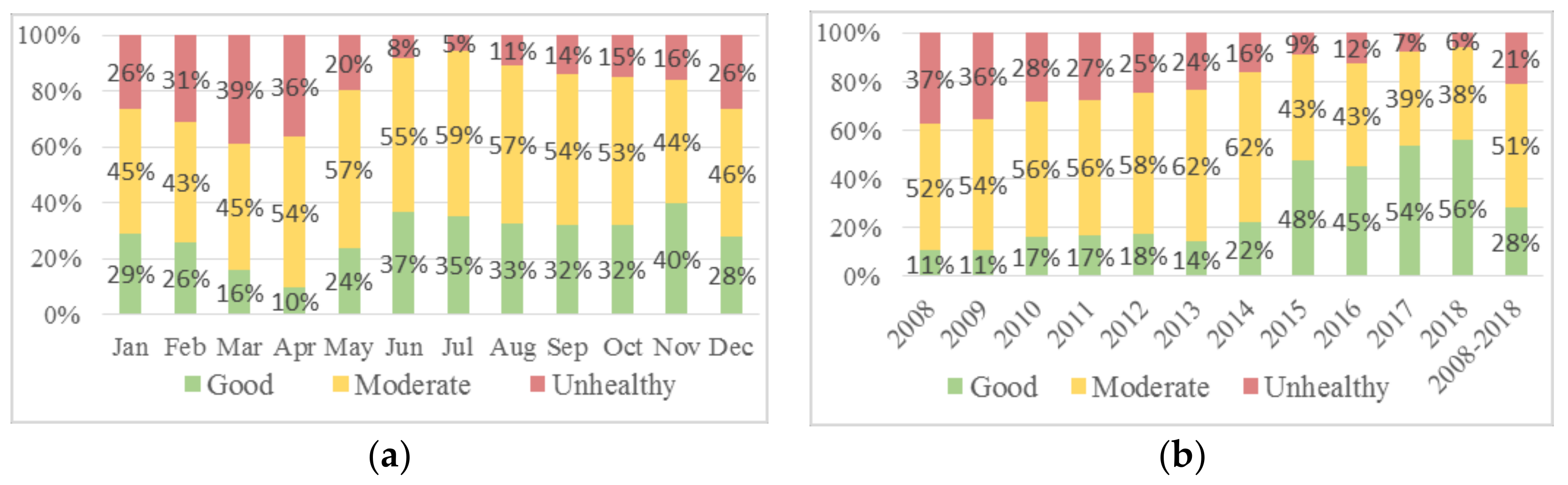
In the Zhongli dataset, moderate is the most frequent AQI level in any given month (Figure 5a). Unhealthy occurs more frequently in December through April, indicating that peak pollution usually occurs in winter and spring. The year-based grouping (Figure 5b) clearly shows a general drop in pollution levels from 2014 to 2018, with a small uptick in 2016. In general, the moderate class accounts for 51% cases while good and unhealthy, respectively, account for 28% and 21%.

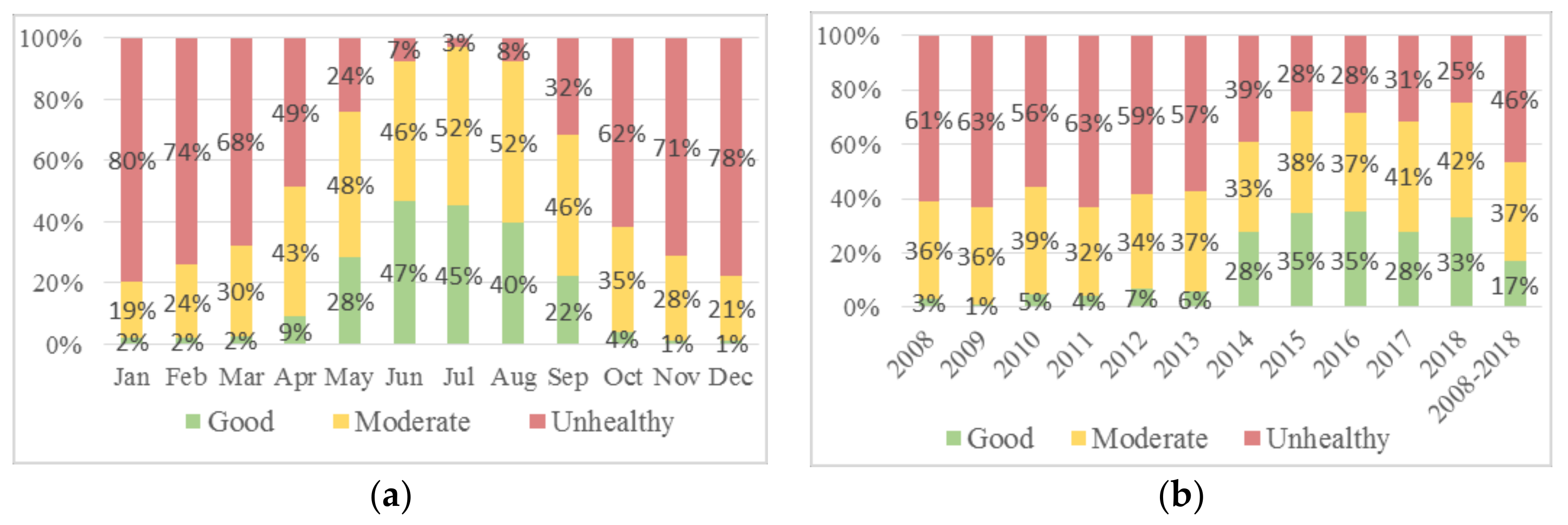
Similar to the Zhongli AQI pattern, pollution in Changhua peaks in March (Figure 6a). However, the degree of air pollution is more severe in Changhua, with unhealthy accounting for 59% of March readings, as opposed to 39% for Zhongli. Like Zhongli, higher AQI levels in Changhua are also clustered in winter and spring, but September, October, and November also featured significant instances of the unhealthy class (respectively 35%, 38%, and 41%). In general, Changhua has poorer air quality than Zhongli, with more frequent AQI > 100 incidents both monthly and annually. However, the full-year AQI readings in Figure 6b show that air quality has gradually improved over time, with a 34% drop in instances of unhealthy from 2008 to 2018.

Southern Taiwan, especially Kaohsiung City, is notorious for its poor air quality due not only to emissions from nearby industrial parks but from particulate matter blowing in from China and Southeast Asia. Figure 7a,b shows significant instances of the unhealthy class (red bars) air quality for most of the year, with reduced pollution levels only in May to September. The worst air quality is concentrated in December and January (respectively 78% and 80% unhealthy).

The winter spike in air pollution is partly due to seasonal atmospheric phenomena that trap air pollution closer to the ground for extended periods. From October to March, Fengshan air quality readings are good less than 5% of the time. In terms of year-based AQI class composition, not much improvement is seen until in 2014–2015 with a sharply declined unhealthy scores after which levels remain relatively stable. Overall, for the 11 years, the Fengshan dataset is dominated by AQI $>$ 100 (46%) followed by 51 $\le$ AQI $\le$ 100 (37%), and AQI $\le$ 50 (17%).

4.2. AQI Prediction Model

Table 3. Parameter Design of ML Methods.

Method		Parameter Design (F1/F8/F24)
		Zhongli	Changhua	Fengshan
Random Forest		No. of Trees = 100/200/200	No. of Trees = 200	No. of Trees = 200/100/200
		m= 4
		Min. observation = 6/6/3	Min. observation = 6/3/3	Min. observation = 6/3/3
AdaBoost		# of Trees= 100
		α = 0.8/0.9999/0.9	α = 0.8/0.9/0.9999	α = 0.8/0.9/0.8
SVM	Linear	C = 3/0.1/0.12, v = 0.5	C = 3/0.12/0.1, v = 0.5	C = 3/0.12/0.1, v = 0.5/0.5/0.9
	Polynomial	C = 3/0.7/0.9, v = 0.5/0.2/0.1, γ = auto, c = 3/5/3, d = 1	C = 3/0.9/0.9, v = 0.5/0.2/0.1, γ = auto, c = 3, d = 1	C =3/0.9/0.9, v = 0.5/0.2/0.9, γ = auto, c = 3, d = 1
	RBF	C = 3/1/1, v = 0.5, γ = auto	C = 3/3/1, v = 0.5, γ = auto	C = 3/3/1, v = 0.5/0.5/0.2, γ = auto
		Max. # of Iterations = 3000
ANN		Activation function: Identity; Optimizer: L-BFGS-B;
		No. of Input neurons = 24; No. of Hidden neurons over layers = 50/50/50; No. of Output neurons = 1
		α = 0.0001; Max. of Iterations = 300
Stacking Ensemble		Regularization: L2 Ridge regression; α = 0.3

specifies the design of the parameters used to generate the prediction models for all dataset (Zhongli, Changhua, and Fengshan). Note that each particular constant for each dataset supposedly contains three values. However, to ease the documentation, any similar value being used across all datasets or at least across different time steps will be written only once. For example, Changhua dataset which uses the number of trees (i.e., 100) in AdaBoost for all time step categories. Additionally, parameter m in the random forest has only one value in all models. To be able to evaluate the ability of each model in accomplishing the task, 80% of data points will be fed into each training process, while the remaining 20% are spared for the testing purpose.

Table 4. Results of ML Algorithms for Zhongli F1-AQI Prediction.

Method	Without Imputation			With Imputation
	RMSE	MAE	R2	RMSE	MAE	R2
SVM-Polynomial	9.836	8.275	0.923	8.145	6.827	0.947
SVM-RBF	9.298	5.119	0.931	8.832	4.617	0.938
SVM-Linear	7.659	6.050	0.953	6.790	5.217	0.963
Random Forest	3.255	2.208	0.992	3.257	2.207	0.992
AdaBoost-Square	3.291	2.187	0.991	3.337	2.185	0.991
AdaBoost-Linear	3.328	2.191	0.991	3.308	2.189	0.991
AdaBoost-Exponential	3.336	2.193	0.991	3.327	2.193	0.991
ANN	3.572	2.438	0.990	3.378	2.396	0.991
Stacking Ensemble	3.236	2.196	0.992	3.243	2.199	0.992

describes the evaluation results of Zhongli F1-AQI prediction using 5 methods with and without imputation. It can be inferred that machine learning algorithms performed very well in predicting future AQI levels in Zhongli for the following hour. The linear kernel is shown to be the best input transformation technique for SVM, with R² results of 0.953 (without imputation) and 0.963 (with imputation). Imputation allows SVM to produce improvement in all evaluation metrics. Furthermore, in terms of MAE score, SVM-RBF outperforms SVM-Linear, but the opposite is true for the RMSE score. This may be due to RBF having more samples with a larger prediction error despite a smaller average error (larger errors produce a greater penalty for RMSE).

The performance of random forest, AdaBoost, ANN, and stacking ensemble algorithm are all comparable. Random forest and stacking ensemble algorithm obtain slightly better R² performance (0.001). Unlike with SVM, imputation does not affect the prediction results for AdaBoost, random forest or the stacking ensemble algorithm, indicating their robustness to missing data. On the other hand, imputation only provides a small degree of improvement on ANN, resulting in tied R² values with AdaBoost. Several loss regression functions (square, linear, exponential) are tested on AdaBoost but without a decisive performance outcome due to efforts to avoid bias since the interpretation could be distorted by randomness, especially given very minor degrees of difference.

Table 5. Results of ML Algorithms for Zhongli F8-AQI Prediction.

Method	Without Imputation			With Imputation
	RMSE	MAE	R2	RMSE	MAE	R2
SVM-Polynomial	24.308	17.981	0.526	23.244	17.135	0.567
SVM-RBF	23.375	17.283	0.562	23.358	17.278	0.563
SVM-Linear	24.262	18.327	0.528	26.674	20.174	0.430
Random Forest	17.471	12.408	0.755	17.477	12.413	0.755
AdaBoost-Square	17.386	11.801	0.758	17.352	11.788	0.759
AdaBoost-Linear	17.273	11.693	0.761	17.221	11.679	0.762
AdaBoost-Exponential	17.283	11.691	0.761	17.284	11.685	0.761
ANN	18.786	13.502	0.717	18.759	13.486	0.718
Stacking Ensemble	17.167	11.804	0.764	17.178	11.799	0.764

summarizes the results for the 8-h Zhongli AQI prediction. The R² value of 0.764 is the best value obtained by the stacking ensemble method. Nonetheless, the performance of SVM becomes worse with an R² value less than 0.6 across all kernels. The values of MAE and RMSE are 17 and 23, respectively. However, ANN and random forest perform better than SVM, with R² scores exceeding 0.7 and error metrics just slightly lower than those obtained with AdaBoost and stacking ensemble. The results match the expectation since the uncertainty increases with the longer period and leads to higher difficulty in the forecast. The study also finds that the overall values are worse than that of the F1-AQI prediction.

Table 6. Results of ML Algorithms for Zhongli F24-AQI Prediction.

Method	Without Imputation			With Imputation
	RMSE	MAE	R2	RMSE	MAE	R2
SVM-Polynomial	33.639	24.799	0.098	34.194	25.034	0.068
SVM-RBF	30.635	23.340	0.252	30.335	23.053	0.267
SVM-Linear	37.001	28.904	0.091	36.835	28.595	0.081
Random Forest	24.974	18.648	0.503	25.007	18.667	0.502
AdaBoost-Square	24.219	16.724	0.533	24.226	16.753	0.532
AdaBoost-Linear	24.039	16.586	0.540	24.074	16.614	0.538
AdaBoost-Exponential	24.053	16.574	0.539	24.099	16.620	0.537
ANN	29.150	21.957	0.323	29.113	21.927	0.325
Stacking Ensemble	23.825	16.667	0.548	23.831	16.693	0.548

shows that no method used for targeting F24-AQI prediction produced an R² score above 0.6, with the lowest score of 0.091. Simply put, the yielded predictions fit the dataset poorly. Stacking ensemble still ranks first, but the R² gap to the second-best method (AdaBoost-Linear) is larger than in the previous cases. SVM performance tracked far behind the other methods with the highest score for evaluation metrics obtained by RBF kernel. However, the R² score is so low that the SVM method is considered not preferable for 24-h prediction.

Predictive model results for F1-AQI Changhua are similar to those for F1-AQI Zhongli. Stacking ensemble, AdaBoost, and random forest provide the best performance for one-hour AQI level prediction (see

Table 7. Results of ML Algorithms for Changhua F1-AQI Prediction.

Method	Without Imputation			With Imputation
	RMSE	MAE	R2	RMSE	MAE	R2
SVM-Polynomial	12.419	11.09	0.907	14.116	12.683	0.880
SVM-RBF	9.672	4.639	0.944	9.596	4.497	0.944
SVM-Linear	9.169	7.055	0.949	10.033	7.638	0.939
Random Forest	3.059	2.055	0.994	3.105	2.066	0.994
AdaBoost-Square	3.093	2.046	0.994	3.126	2.054	0.994
AdaBoost-Linear	3.089	2.043	0.994	3.115	2.048	0.994
AdaBoost-Exponential	3.093	2.046	0.994	3.126	2.054	0.994
ANN	3.914	2.505	0.991	3.870	2.541	0.991
Stacking Ensemble	3.039	2.043	0.994	3.076	2.057	0.994

). These algorithms perform better for all evaluation metrics in Changhua than in Zhongli. Also, the imputation process reduces the performance of SVM, but not the other algorithms.

When it comes to the F8-AQI prediction (as shown in

Table 8. Results of ML Algorithms for Changhua F8-AQI Prediction.

Method	Without Imputation			With Imputation
	RMSE	MAE	R2	RMSE	MAE	R2
SVM-Polynomial	26.225	20.082	0.585	25.818	19.919	0.598
SVM-RBF	25.548	19.422	0.606	25.730	19.597	0.600
SVM-Linear	31.189	23.412	0.413	25.628	19.623	0.603
Random Forest	18.435	13.711	0.795	18.423	13.707	0.795
AdaBoost-Square	17.877	12.747	0.807	17.871	12.734	0.807
AdaBoost-Linear	17.825	12.732	0.808	17.810	12.718	0.809
AdaBoost-Exponential	17.822	12.733	0.808	17.815	12.729	0.808
ANN	20.451	15.329	0.748	20.312	15.213	0.751
Stacking Ensemble	17.801	12.855	0.809	17.792	12.856	0.809

), the Changhua prediction again outperforms that of Zhongli. AdaBoost and stacking ensemble both yield R² scores exceeding 0.8. Without imputation, stacking ensemble outperforms the other methods. However, with imputation, AdaBoost performance is comparable to that of stacking ensemble. SVM-linear gives the highest MAE and RMSE results, i.e., 23.412 and 31.189, respectively. These error metrics can be further reduced to 19.623 and 25.628 by imputation.

In the Zhongli dataset, the time step selection affects the performance of machine learning methods, and this is consistent with the results for the F24-AQI prediction models in Changhua (

Table 9. Results of ML Algorithms for Changhua F24-AQI Prediction.

Method	Without Imputation			With Imputation
	RMSE	MAE	R2	RMSE	MAE	R2
SVM-Polynomial	40.662	31.689	0.006	41.834	32.727	0.052
SVM-RBF	34.879	26.977	0.269	34.852	26.948	0.270
SVM-Linear	37.451	29.047	0.157	37.092	28.703	0.173
Random Forest	26.765	20.281	0.570	26.786	20.299	0.569
AdaBoost-Square	26.282	18.781	0.585	26.288	18.799	0.585
AdaBoost-Linear	25.786	18.204	0.600	25.817	18.246	0.599
AdaBoost-Exponential	25.747	18.144	0.602	25.773	18.185	0.601
ANN	30.919	23.753	0.426	30.803	23.647	0.430
Stacking Ensemble	25.630	18.255	0.605	25.655	18.294	0.604

). Declination occurs across all models with a very low R². The SVM-Polynomial gives the worst performance for the imputed dataset and an MAE value exceeding 30, and an RMSE value exceeding 40. The best performance is still obtained by the stacking ensemble method, with an R² score of 0.605, and MAE and RMSE values respectively below 19 and 26. Among all kernels used by SVM, the radial basis function appears to be the most effective for 24-h AQI predictions. Moreover, AdaBoost-exponential slightly underperforms stacking ensemble in terms of R² and RMSE, but consistently provides better MAE results.

Table 10. Results of ML Algorithms for Fengshan F1-AQI Prediction.

Method	Without Imputation			With Imputation
	RMSE	MAE	R2	RMSE	MAE	R2
SVM-Polynomial	7.072	5.556	0.974	7.275	5.821	0.973
SVM-RBF	9.119	5.542	0.957	8.324	4.702	0.964
SVM-Linear	9.529	7.400	0.953	8.485	6.621	0.963
Random Forest	2.971	1.869	0.995	2.979	1.868	0.995
AdaBoost-Square	3.020	1.771	0.995	2.996	1.766	0.995
AdaBoost-Linear	2.995	1.767	0.995	2.983	1.760	0.995
AdaBoost-Exponential	3.020	1.771	0.995	2.996	1.766	0.995
ANN	3.966	2.544	0.992	3.821	2.585	0.992
Stacking Ensemble	2.925	1.823	0.996	2.921	1.814	0.996

summarizes the results for the one-hour prediction model without and with k-NN imputation step in the Fengshan dataset. Stacking ensemble learning outperforms other techniques in terms of RMSE and R², while SVM obtains the worst performance in every prediction case. However, imputation slightly enhances the results, particularly for the RBF and linear kernels, but not for the polynomial kernel which shows a performance decline using the imputed dataset. Also note that while comparing with the results in the other two cities, Zhongli and Changhua, Fengshan shows the best performance in all evaluation measures.

In terms of eight-hour prediction, imputation has a significant impact on SVM-Linear, increasing R² from 0.318 to 0.546 (as shown in

Table 11. Results of ML Algorithms for Fengshan F8-AQI Prediction.

Method	Without Imputation			With Imputation
	RMSE	MAE	R2	RMSE	MAE	R2
SVM-Polynomial	25.658	19.806	0.659	25.512	19.606	0.663
SVM-RBF	25.810	20.392	0.655	25.665	20.248	0.659
SVM-Linear	36.292	26.859	0.318	29.598	23.028	0.546
Random Forest	16.634	12.111	0.857	16.606	12.100	0.857
AdaBoost-Square	16.440	11.399	0.860	16.498	11.391	0.859
AdaBoost-Linear	16.367	11.364	0.861	16.339	11.367	0.862
AdaBoost-Exponential	16.387	11.373	0.861	16.398	11.367	0.861
ANN	19.112	14.285	0.811	18.975	14.182	0.814
Stacking Ensemble	16.302	11.517	0.862	16.279	11.527	0.863

). RMSE and MAE are also improved by 10% and shift closer to the performance of other SVM kernels. Of the three locations, application of machine learning algorithms has the biggest impact on 8-h predictions in Fengshan, with stacking ensemble providing the greatest improvement, followed by AdaBoost, random forest, ANN, and SVM. This sequence is consistent for all results.

As summarized in

Table 12. Results of ML Algorithms for Fengshan F24-AQI Prediction.

Method	Without Imputation			With Imputation
	RMSE	MAE	R2	RMSE	MAE	R2
SVM-Polynomial	35.203	28.025	0.357	35.330	28.140	0.353
SVM-RBF	37.696	30.300	0.263	35.368	28.485	0.351
SVM-Linear	35.954	28.520	0.329	36.511	28.763	0.309
Random Forest	23.388	17.476	0.716	23.384	17.485	0.716
AdaBoost-Square	22.935	15.932	0.727	22.927	15.939	0.727
AdaBoost-Linear	22.663	15.743	0.734	22.654	15.753	0.734
AdaBoost-Exponential	22.708	15.777	0.733	22.723	15.790	0.732
ANN	27.008	20.542	0.622	26.882	20.416	0.625
Stacking Ensemble	22.872	16.372	0.729	22.618	16.105	0.735

, for the 24-h predictions in Fengshan, while overall SVM results are not promising, the other methods show quite acceptable evaluation scores. The top three methods (stacking ensemble, AdaBoost, and random forest) obtained R² scores exceeding 0.71 for which the MAE and RMSE results are comparable to the F8-AQI prediction for Fengshan. Surprisingly, the stacking ensemble is found to be affected by imputation but, even with imputation, the MAE value is still higher than that of all AdaBoost versions (linear, square, and exponential). AdaBoost and stacking ensemble show consistent results, and AdaBoost generally obtains worse RMSE and R² but better MAE.

4.3. Implementation of AQI Forecasting Model

This section describes a simulation-like AQI forecasting using stacking ensemble and AdaBoost (the two best methods from the analyses in Section 4.2) as backend techniques. Each prediction is accompanied by a prediction interval (PI) within a 95% confidence level, which describes a given tolerance for the prediction value such that there is 95% chance that the actual observation could fall within this range. The prediction interval is calculated using the formula below [21]:

$$PI=z_{\alpha ∕2}\times \sigma \left(3\right)$$

(3)

where $\sigma$ represents the standard deviation of the residual errors defined as [22]:

$$\sigma = \sqrt{\frac{1}{n-2}{\displaystyle \sum }_{i=1}^n{(y_i-{\widehat{y}}_i)}^2}$$

(4)

Prediction intervals that reflect the uncertainty of a model’s output should be adjusted dynamically as new observations are received every hour, thus ensuring that the prediction interval is always current. The one-month samples (December 2018) from the Zhongli dataset are used to obtain the standard deviation.

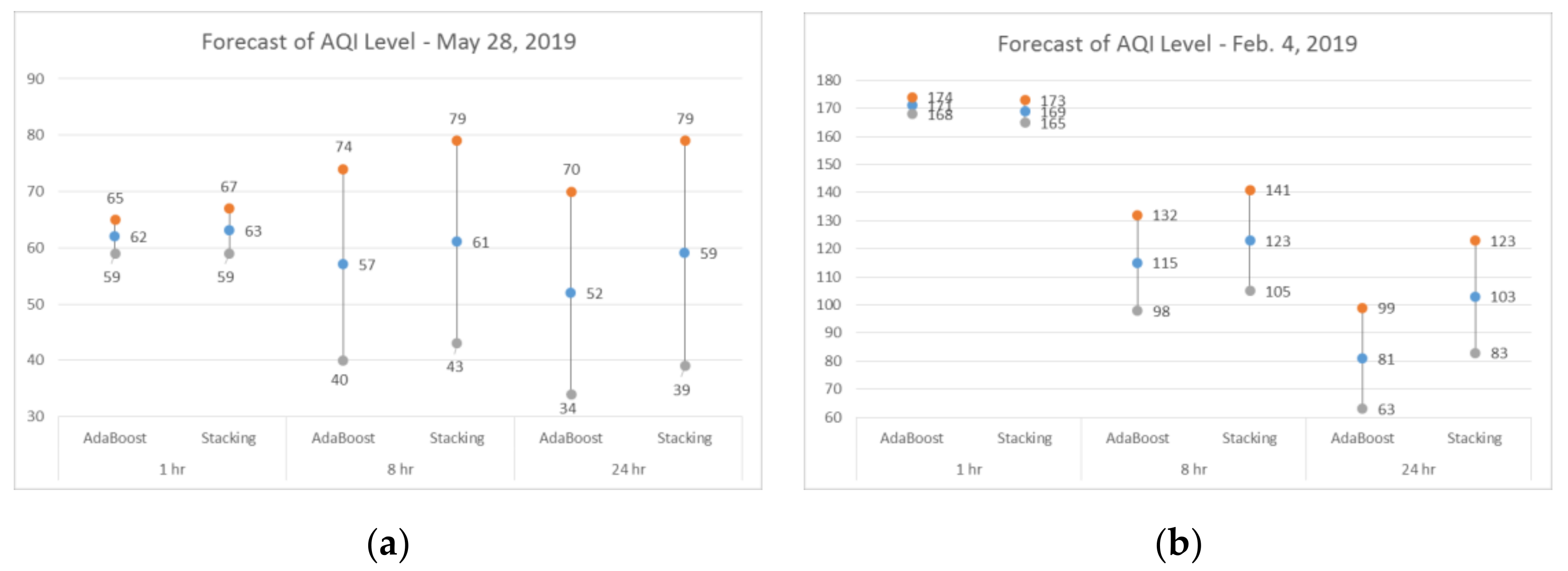
As shown in Figure 8a, the higher the prediction time step, the wider the tolerance needed to represent the estimation. AdaBoost and stacking ensemble outperform the other techniques tested in the previous section, obtaining similar predictions and prediction intervals. The predictions here are all based on authentic data, where the best models in each prediction category are reused. Figure 8b shows another forecast constructed during winter, providing an example of poor air quality cases captured in the prediction of F1-AQI, F8-AQI, and F24-AQI using AdaBoost and stacking ensemble.

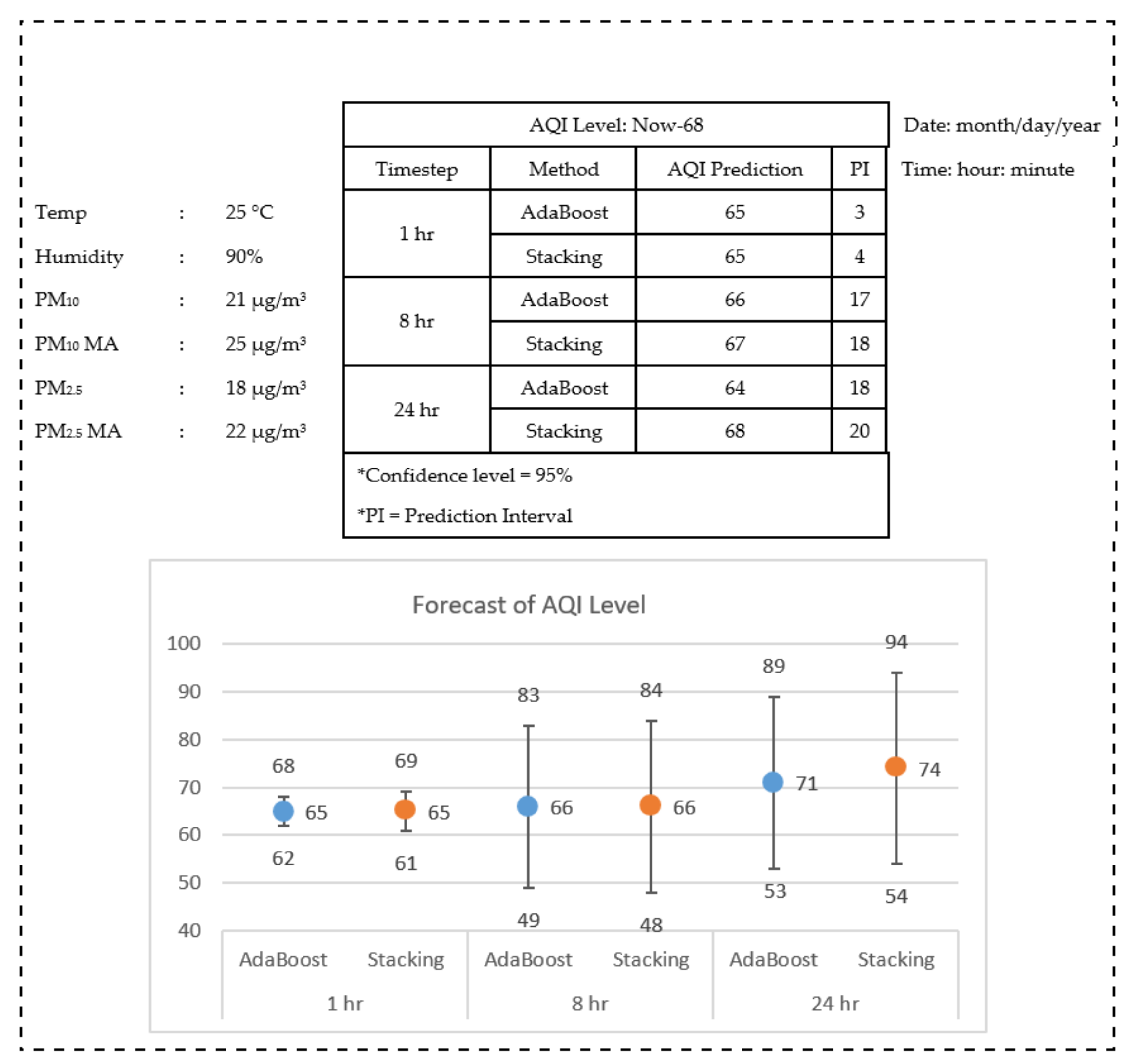
Figure 9 provides an illustration on how the information will be provided and visualized given a sample of upcoming data for the monitoring and forecasting of the air quality. Noted that as shown by the graph, the higher the time step of prediction the wider the tolerance needed to escort the estimation. AdaBoost and stacking are two methods that outperform other techniques tested in the previous section. Their predictions are close to each other and so are the prediction intervals. The predictions here are based on the real scheme, where the best models of them in each category of prediction were reused again by incorporating the actual values from 24 features.

5. Conclusions

Applying artificial intelligence methods provides promising results for AQI forecasting. This study obtained data collected by EPA and CWB of Taiwan over 11 years. Three regions (North: Zhongli, Central: Changhua, South: Fengshan) in Taiwan were considered, including two notorious places (Changhua and Fengshan) for their bad air quality all year round. With good results for R², stacking ensemble and AdaBoost offer the best performance of target predictions based on three different datasets. To be more specific, the stacking ensemble delivers the best RMSE results, while AdaBoost provides the best MAE results. All results show that SVM yields the worst results among all methods explored, and only provides meaningful results for 1-h predictions. The results also confirm that the two machine learning methods, AdaBoost and stacking ensemble, employed in this study can outperform popular methods in the literature, such as SVM, random forest, and ANN. In other words, AdaBoost and stacking ensemble can be considered new and superior alternatives for AQI forecast.

This study also indicates that prediction performance varies over different regions in Taiwan. Comparing results from datasets sourced from three different regions displays best results for Fengshan AQI prediction (Southern Taiwan), where performance decay with increased time step is less pronounced than those in Zhongli (north) and Changhua (central). Also, 95% confidence intervals for 1-h, 8-h and 24-h forecast are calculated, respectively. Compared to the single value prediction, the 95% C.I. can provide a better reference to the decision-maker. For example, an event planner can decide if the outdoor activities can go on based on the air quality forecast with better confidence. Future work should focus on improving performance using stacking ensemble, AdaBoost and random forest with hyperparameter optimization, particularly for predictions with larger time steps (F8-AQI and F24-AQI).

References

1. World Health Organization. Air Pollution. Available online: https://www.who.int/health-topics/air-pollution#tab=tab_1/ (accessed on 13 March 2020).
2. Ghorani-Azam, A.; Riahi-Zanjani, B.; Balali-Mood, M. Effects of Air Pollution on Human Health and Practical Measures for Prevention in Iran. J. Res. Med. Sci. 2016, 21, 1–12. [Google Scholar]
3. Conticini, E.; Frediani, B.; Caro, D. Can Atmospheric Pollution Be Considered a Co-factor in Extremely High Level of SARS-CoV-2 Lethality in Northern Italy? Environ. Pollut. 2020, 261, 114465. [Google Scholar] [CrossRef] [PubMed]
4. Rybarczyk, Y.; Zalakeviciute, R. Machine Learning Approaches for Outdoor Air Quality Modelling: A Systematic Review. Appl. Sci. 2018, 8, 2570. [Google Scholar] [CrossRef] [Green Version]
5. Raimondo, G.; Montuori, A.; Moniaci, W.; Pasero, E.; Almkvist, E. A Machine Learning Tool to Forecast PM10 Level. In Proceedings of the Fifth Conference on Artificial Intelligence Applications to Environmental Science, San Antonio, TX, USA, 14–18 January 2007; pp. 1–9. [Google Scholar]
6. Garcia, J.M.; Teodoro, F.; Cerdeira, R.; Coelho, R.M.; Kumar, P.; Carvalho, M.G. Developing a Methodology to Predict PM10 Concentrations in Urban Areas Using Generalized Linear Models. Environ. Technol. 2016, 37, 2316–2325. [Google Scholar] [CrossRef] [PubMed] [Green Version]
7. Park, S.; Kim, M.; Kim, M.; Namgung, H.-G.; Kim, K.-T.; Cho, K.H.; H, K.; Kwon, S.-B. Predicting PM10 Concentration in Seoul Metropolitan Subway Stations Using Artificial Neural Network (ANN). J. Hazard. Mater. 2018, 341, 75–82. [Google Scholar] [CrossRef] [PubMed]
8. Yu, R.; Yang, Y.; Yang, L.; Han, G.; Move, O.A. RAQ A Random Forest Approach for Predicting Air Quality in Urban Sensing Systems. Sensors 2016, 16, 86. [Google Scholar] [CrossRef] [PubMed] [Green Version]
9. Yi, X.; Zhang, J.; Wang, Z.; Li, T.; Zheng, Y. Deep Distributed Fusion Network for Air Quality Prediction. In Proceedings of the 24th ACM SIGKDD International Conference on Knowledge Discovery and Data Mining, London, UK, 19–23 August 2018; pp. 965–973. [Google Scholar]
10. Veljanovska, K.; Dimoski, A. Air Quality Index Prediction Using Simple Machine Learning Algorithms. Int. J. Emerg. Trends Technol. Comput. Sci. 2018, 7, 25–30. [Google Scholar]
11. Muhammad, I.; Yan, Z. Supervised Machine Learning Approaches: A Survey. Ictact J. Soft Comput. 2015, 5, 946–952. [Google Scholar] [CrossRef]
12. Awad, M.; Khanna, R. Support Vector Regression. In Efficient Learning Machines; Apress: Berkeley, CA, USA, 2015. [Google Scholar]
13. Schölkopf, B.; Smola, A.J.; Williamson, R.; Bartlett, P. New Support Vector Algorithms. Neural Comput. 2000, 12, 1207–1245. [Google Scholar] [CrossRef] [PubMed]
14. Chang, C.-C.; Lin, C.-J. Training ν-Support Vector Regression: Theory and Algorithms. Neural Comput. 2002, 14, 1959–1977. [Google Scholar] [CrossRef] [PubMed]
15. Wu, X.; Srihari, R. New v-Support Vector Machines and Their Sequential Minimal Optimization. In Proceedings of the Twentieth International Conference on Machine Learning, Washington, DC, USA, 21–24 August 2003; AAAI Press: Washington, DC, USA, 2003; pp. 824–831. [Google Scholar]
16. Yu, L.; Wang, S.; Lai, K.K. Basic Learning Principles of Artificial Neural Networks. In Foreign-Exchange-Rate Forecasting With Artificial Neural Networks; Yu, L., Wang, S., Lai, K.K., Eds.; Springer: Boston, MA, USA, 2007; pp. 27–37. [Google Scholar]
17. Rocca, J. Ensemble Methods: Bagging, Boosting and Stacking. Available online: https://towardsdatascience.com/ensemble-methods-bagging-boosting-and-stacking-c9214a10a205 (accessed on 23 April 2019).
18. Taiwan’s Environmental Protection Administration. Taiwan Air Quality Monitoring Network. Available online: https://taqm.epa.gov.tw/taqm/en/b0201.aspx (accessed on 13 March 2020).
19. Iskandaryan, D.; Ramos, F.; Trilles, S. Air Quality Prediction in Smart Cities Using Machine Learning Technologies Based on Sensor Data: A Review. Appl. Sci. 2020, 10, 2401. [Google Scholar] [CrossRef] [Green Version]
20. Dufour, J.M. Coefficients of Determination; McGill University: Québec, QC, Canada, 2011. [Google Scholar]
21. Brownlee, J. Prediction Intervals for Machine Learning. Available online: https://machinelearningmastery.com/prediction-intervals-for-machine-learning/ (accessed on 30 May 2018).
22. Shrestha, D.L.; Solomatine, D.P. Machine Learning Approaches for Estimation of Prediction Interval for the Model Output. Neural Netw. 2006, 19, 225–235. [Google Scholar] [CrossRef] [PubMed]
Figure 1. Overview of SVM algorithm: (a) SVM for classification; (b) SVM for regression.
Applsci 10 09151 g001
Figure 2. Illustration of a random forest algorithm.
Applsci 10 09151 g002
Figure 3. Illustration of artificial neural network.
Applsci 10 09151 g003
Figure 4. Demonstration of linear regression’s learning process.
Applsci 10 09151 g004
Figure 5. Composition of AQI classes in Zhongli: (a) Month-based; (b) Year-based and Overall-based.
Applsci 10 09151 g005
Figure 6. Composition of AQI classes in Changhua: (a) Month-based; (b) Year-based and Overall-based.
Applsci 10 09151 g006
Figure 7. Composition of AQI classes in Fengshan: (a) Month-based; (b) Year-based and Overall-based.
Applsci 10 09151 g007
Figure 8. Forecast of AQI: (a) on 28 May 2019, 07:00; (b) on 4 February 2019, 03:00.
Applsci 10 09151 g008
Figure 9. Illustration of Air Quality Monitoring and Forecasting System.
Applsci 10 09151 g009