Non-Intrusive Load Disaggregation Based on a Multi-Scale Attention Residual Network


Abstract
1. Introduction
2. Multi-Scale Attention Residual Network
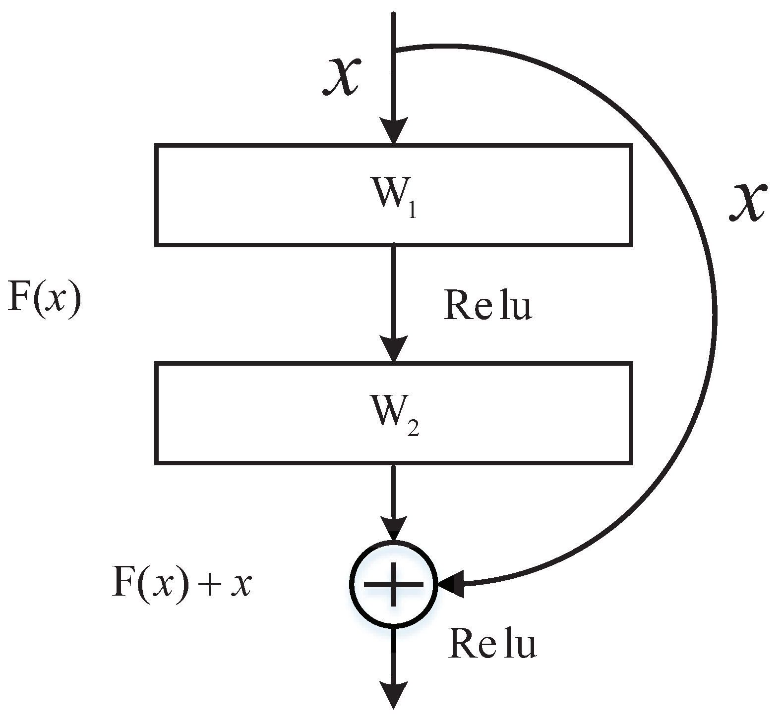
2.1. Deep Residual Network
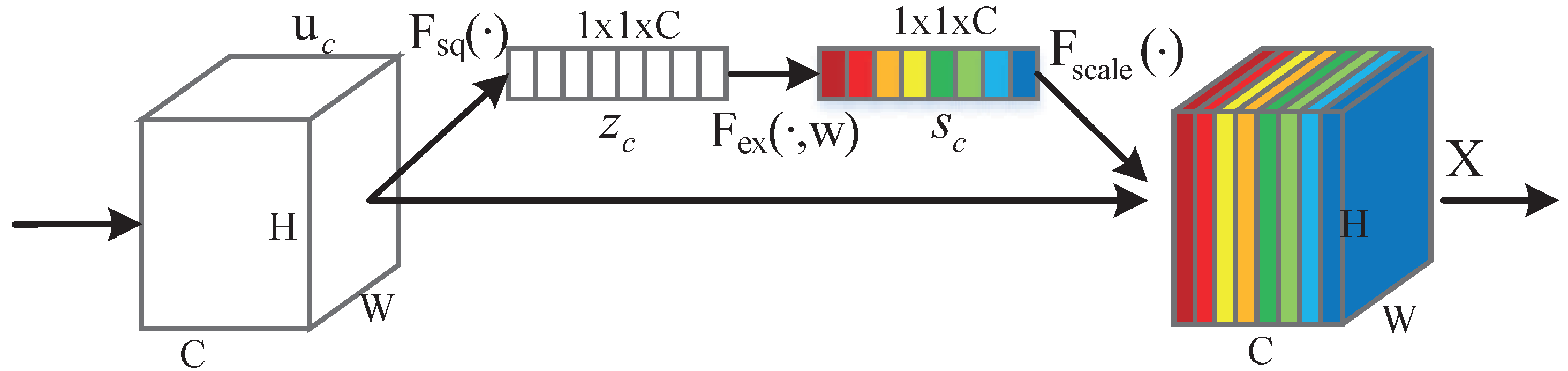
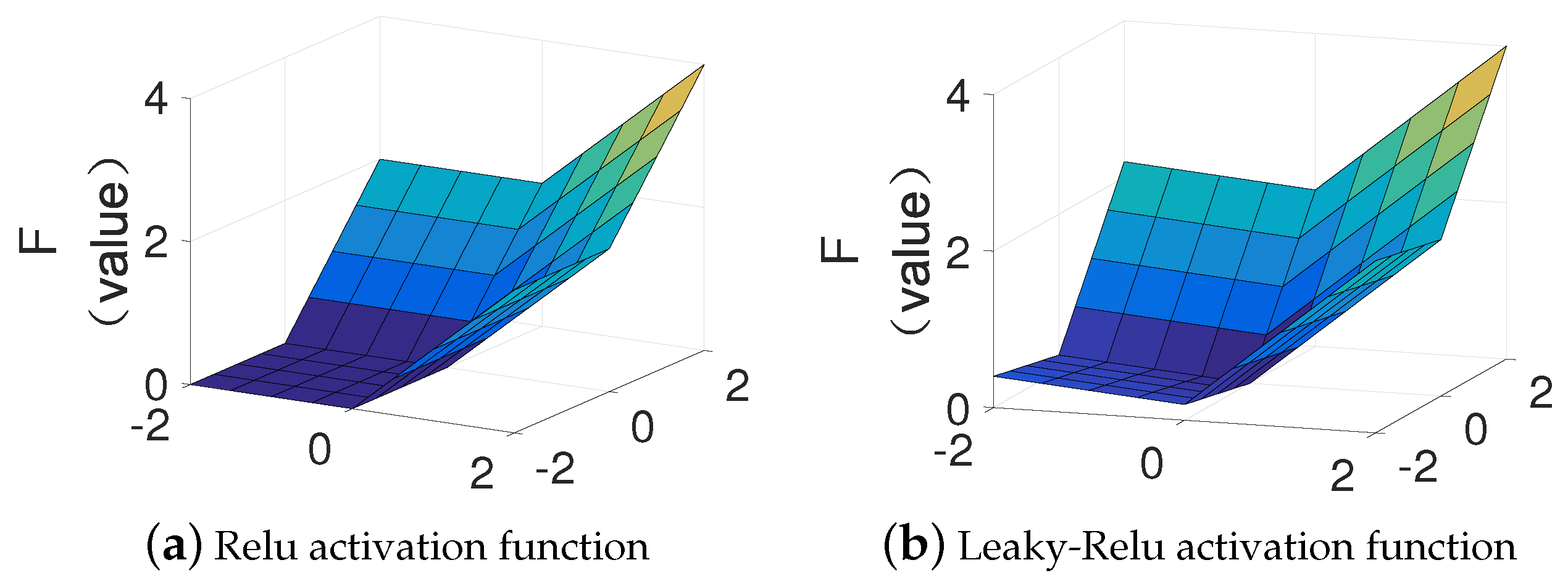
2.2. Attention Mechanism
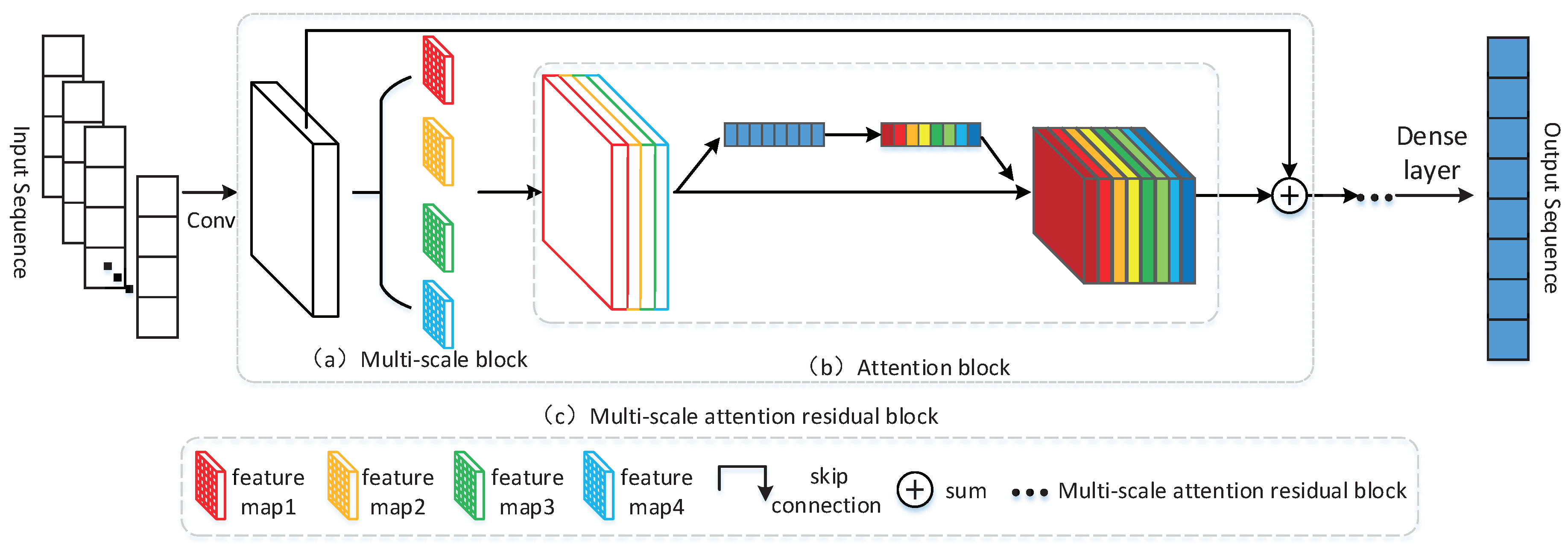
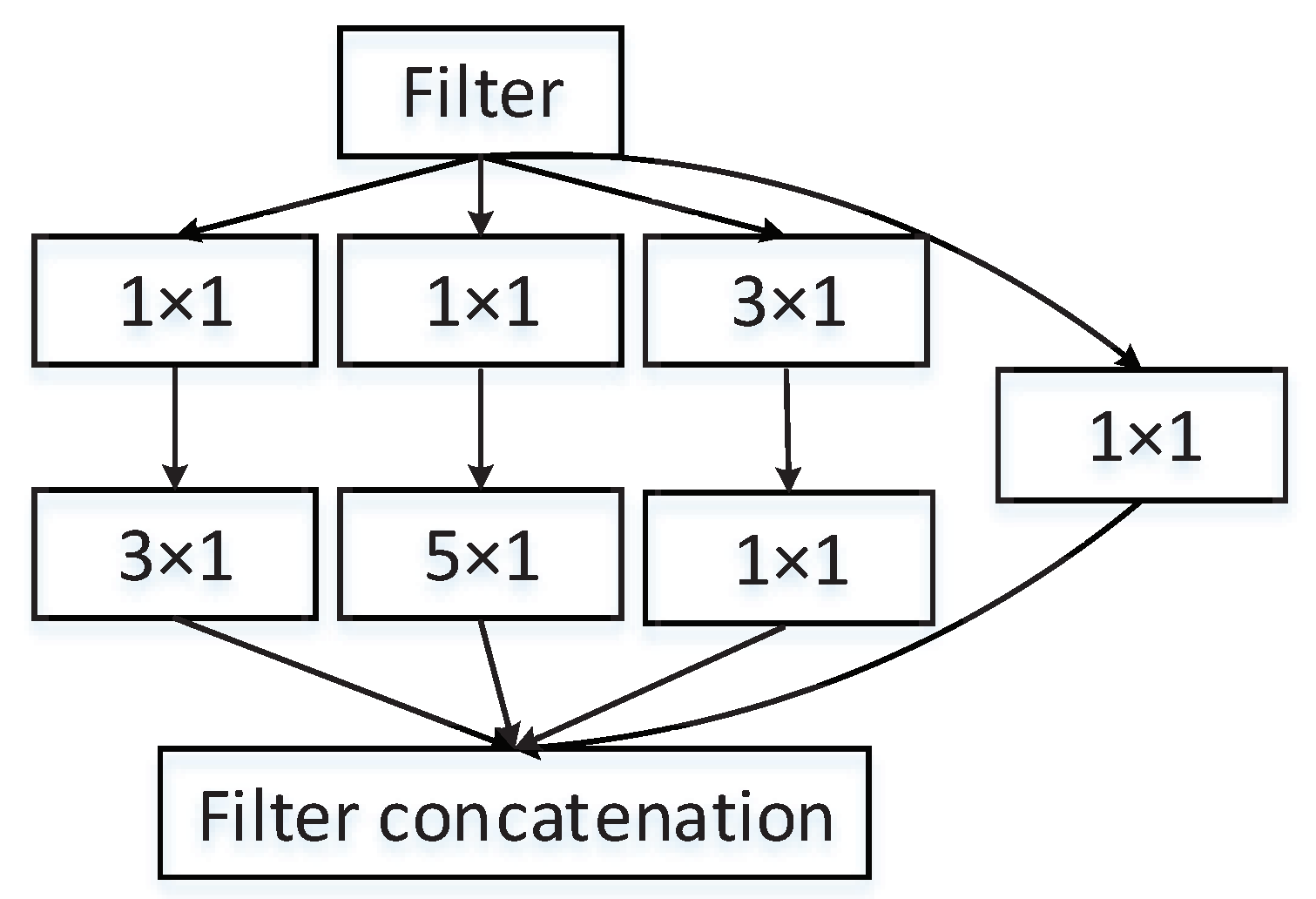
2.3. Multi-Scale Attention Resnet Based NILD
3. Data Selection and Preprocessing
3.1. Data Sources
3.2. Data Preprocessing
3.3. Sliding Window
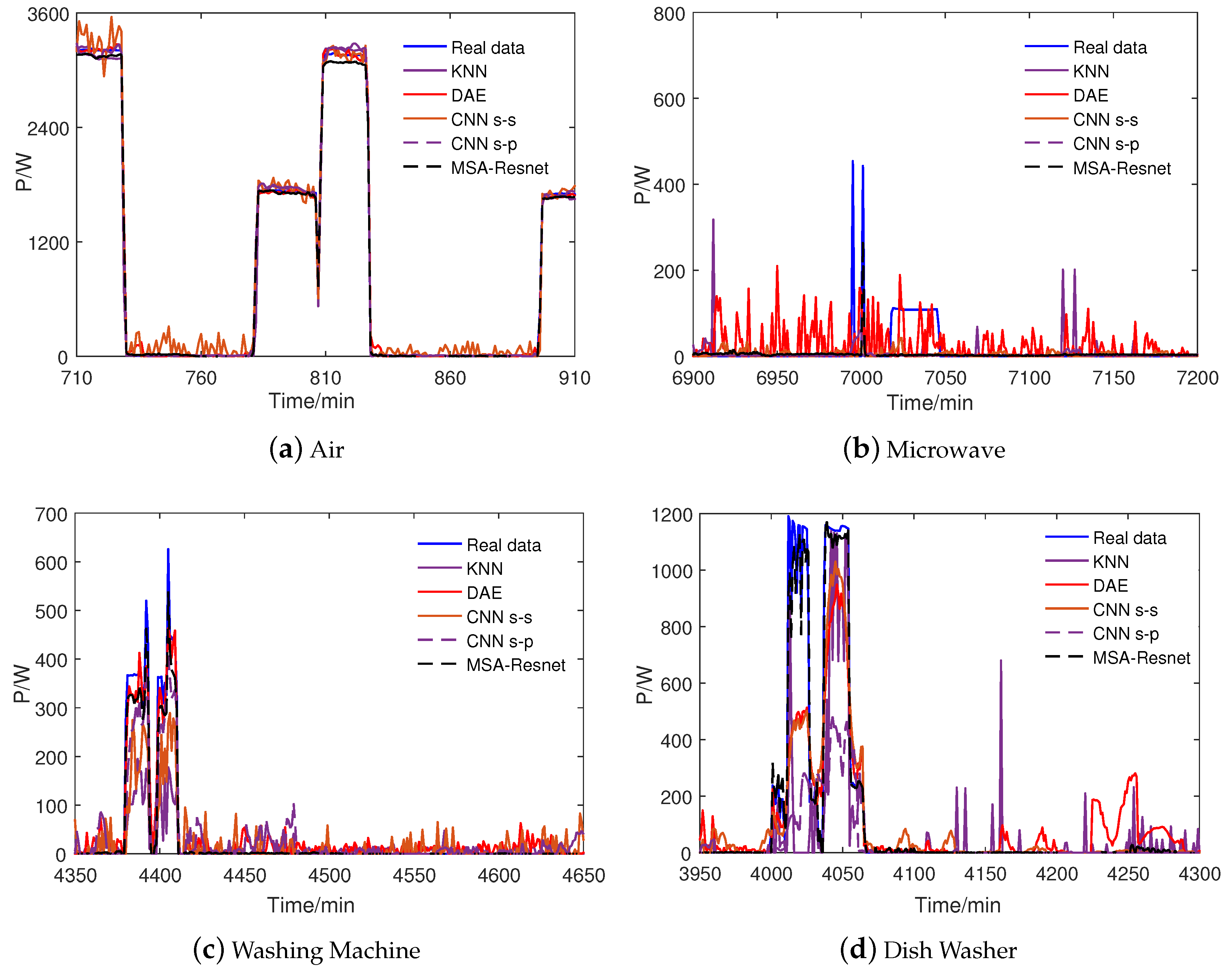
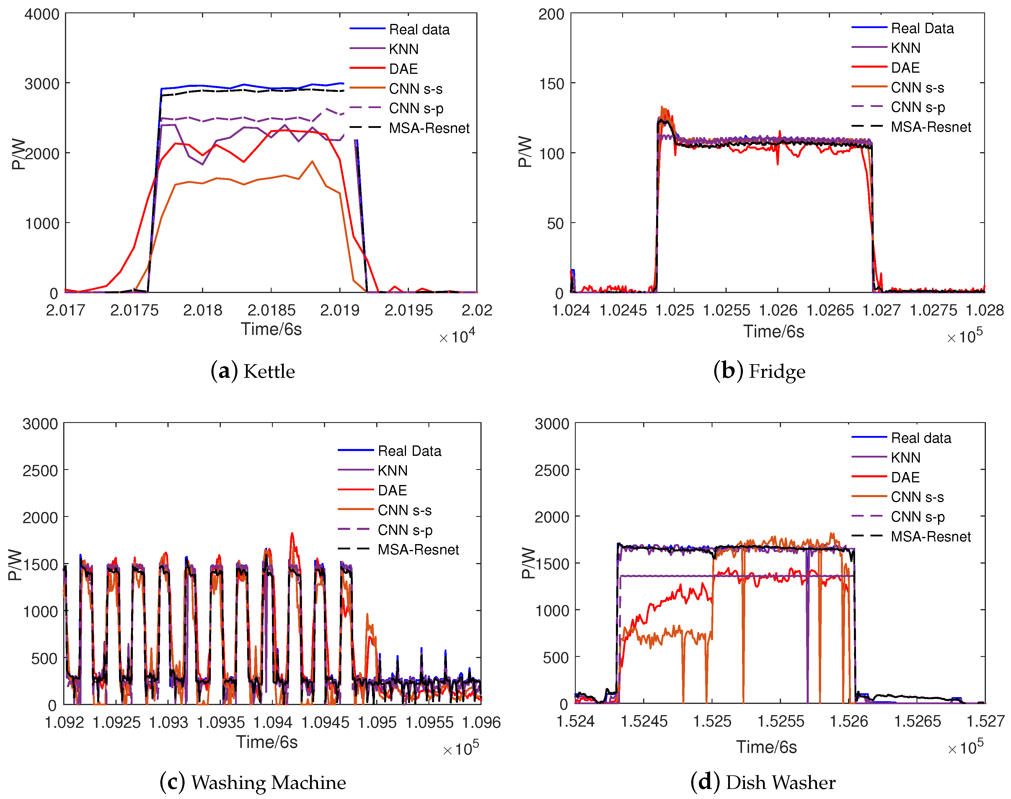
4. Result
5. Conclusions
Author Contributions
Funding
Acknowledgments
Conflicts of Interest
References
- Wong, Y.F.; Şekercioğlu, Y.A.; Drummond, T.; Wong, V.S. Recent approaches to non-intrusive load monitoring techniques in residential settings. In Proceedings of the 2013 IEEE Computational Intelligence Applications in Smart Grid, Singapore, 16–19 April 2013; pp. 73–79. [Google Scholar]
- Prada, J.; Dorronsoro, J.R. General noise support vector regression with non-constant uncertainty intervals for solar radiation prediction. J. Mod. Power Syst. Clean Energy 2018, 6, 268–280. [Google Scholar] [CrossRef]
- Liu, H.; Zeng, P.; Guo, J.; Wu, H.; Ge, S. An optimization strategy of controlled electric vehicle charging considering demand side response and regional wind and photovoltaic. J. Mod. Power Syst. Clean Energy 2015, 3, 232–239. [Google Scholar] [CrossRef]
- Tostado-Véliz, M.; Arévalo, P.; Jurado, F. A Comprehensive Electrical-Gas-Hydrogen Microgrid Model for Energy Management Applications. Energy Convers. Manag. 2020, 228, 113726. [Google Scholar] [CrossRef]
- Hart, G.W. Nonintrusive appliance load monitoring. Proc. IEEE 1992, 80, 1870–1891. [Google Scholar] [CrossRef]
- Rahimpour, A.; Qi, H.; Fugate, D.; Kuruganti, T. Non-intrusive energy disaggregation using non-negative matrix factorization with sum-to-k constraint. IEEE Trans. Power Syst. 2017, 32, 4430–4441. [Google Scholar] [CrossRef]
- Zoha, A.; Gluhak, A.; Imran, M.A.; Rajasegarar, S. Non-intrusive load monitoring approaches for disaggregated energy sensing: A survey. Sensors 2012, 12, 16838–16866. [Google Scholar] [CrossRef]
- Chang, H.H.; Lin, L.S.; Chen, N.; Lee, W.J. Particle-swarm-optimization-based nonintrusive demand monitoring and load identification in smart meters. IEEE Trans. Ind. Appl. 2013, 49, 2229–2236. [Google Scholar] [CrossRef]
- Lin, Y.H.; Tsai, M.S. Development of an improved time–frequency analysis-based nonintrusive load monitor for load demand identification. IEEE Trans. Instrum. Meas. 2013, 63, 1470–1483. [Google Scholar] [CrossRef]
- Piga, D.; Cominola, A.; Giuliani, M.; Castelletti, A.; Rizzoli, A.E. Sparse optimization for automated energy end use disaggregation. IEEE Trans. Control Syst. Technol. 2015, 24, 1044–1051. [Google Scholar] [CrossRef]
- Batra, N.; Singh, A.; Whitehouse, K. Neighbourhood nilm: A big-data approach to household energy disaggregation. arXiv 2015, arXiv:1511.02900. [Google Scholar]
- Tsai, M.S.; Lin, Y.H. Modern development of an adaptive non-intrusive appliance load monitoring system in electricity energy conservation. Appl. Energy 2012, 96, 55–73. [Google Scholar] [CrossRef]
- Kolter, J.; Batra, S.; Ng, A. Energy disaggregation via discriminative sparse coding. Adv. Neural Inf. Process. Syst. 2010, 23, 1153–1161. [Google Scholar]
- Johnson, M.J.; Willsky, A.S. Bayesian nonparametric hidden semi-Markov models. J. Mach. Learn. Res. 2013, 14, 673–701. [Google Scholar]
- Kim, H.; Marwah, M.; Arlitt, M.; Lyon, G.; Han, J. Unsupervised disaggregation of low frequency power measurements. In Proceedings of the 2011 SIAM International Conference on Data Mining, Society for Industrial and Applied Mathematics, Mesa, AZ, USA, 28–30 April 2011; pp. 747–758. [Google Scholar]
- Saitoh, T.; Osaki, T.; Konishi, R.; Sugahara, K. Current sensor based home appliance and state of appliance recognition. SICE J. Control Meas. Syst. Integr. 2010, 3, 86–93. [Google Scholar] [CrossRef]
- Hassan, T.; Javed, F.; Arshad, N. An empirical investigation of VI trajectory based load signatures for non-intrusive load monitoring. IEEE Trans. Smart Grid 2013, 5, 870–878. [Google Scholar] [CrossRef]
- Xia, M.; Wang, K.; Zhang, X.; Xu, Y. Non-intrusive load disaggregation based on deep dilated residual network. Electr. Power Syst. Res. 2019, 170, 277–285. [Google Scholar] [CrossRef]
- Xia, M.; Zhang, X.; Weng, L.; Xu, Y. Multi-Stage Feature Constraints Learning for Age Estimation. IEEE Trans. Inf. Forensics Secur. 2020, 15, 2417–2428. [Google Scholar] [CrossRef]
- Kuo, P.H.; Huang, C.J. A high precision artificial neural networks model for short-term energy load forecasting. Energies 2018, 11, 213. [Google Scholar] [CrossRef]
- Kelly, J.; Knottenbelt, W. Neural nilm: Deep neural networks applied to energy disaggregation. In Proceedings of the 2nd ACM International Conference on Embedded Systems for Energy-Efficient Built Environments, Seoul, Korea, 4–5 November 2015; pp. 55–64. [Google Scholar]
- Zhang, C.; Zhong, M.; Wang, Z.; Goddard, N.; Sutton, C. Sequence-to-point learning with neural networks for nonintrusive load monitoring. arXiv 2016, arXiv:1612.09106. [Google Scholar]
- Liu, Y.; Liu, Y.; Liu, J.; Li, M.; Ma, Z.; Taylor, G. High-performance predictor for critical unstable generators based on scalable parallelized neural networks. J. Mod. Power Syst. Clean Energy 2016, 4, 414–426. [Google Scholar] [CrossRef]
- Yang, Y.; Zhong, J.; Li, W.; Gulliver, T.A.; Li, S. Semi-Supervised Multi-Label Deep Learning based Non-intrusive Load Monitoring in Smart Grids. IEEE Trans. Ind. Inform. 2019, 16, 6892–6902. [Google Scholar] [CrossRef]
- Yadav, A.; Sinha, A.; Saidi, A.; Trinkl, C.; Zörner, W. NILM based Energy Disaggregation Algorithm for Dairy Farms. In Proceedings of the 5th International Workshop on Non-Intrusive Load Monitoring, Yokohama, Japan, 18 November 2020; pp. 16–19. [Google Scholar]
- Faustine, A.; Pereira, L.; Bousbiat, H.; Kulkarni, S. UNet-NILM: A Deep Neural Network for Multi-tasks Appliances State Detection and Power Estimation in NILM. In Proceedings of the 5th International Workshop on Non-Intrusive Load Monitoring, Yokohama, Japan, 18 November 2020; pp. 84–88. [Google Scholar]
- Jin, Y.; Guo, H.; Wang, J.; Song, A. A Hybrid System Based on LSTM for Short-Term Power Load Forecasting. Energies 2020, 13, 6241. [Google Scholar] [CrossRef]
- de Paiva Penha, D.; Castro, A.R.G. Home appliance identification for NILM systems based on deep neural networks. Int. J. Artif. Intell. Appl. 2018, 9, 69–80. [Google Scholar] [CrossRef]
- He, K.; Zhang, X.; Ren, S.; Sun, J. Deep residual learning for image recognition. In Proceedings of the IEEE Conference on Computer Vision and Pattern Recognition, Las Vegas, NV, USA, 27–30 June 2016; pp. 770–778. [Google Scholar]
- Wang, F.; Jiang, M.; Qian, C.; Yang, S.; Li, C.; Zhang, H.; Wang, X.; Tang, X. Residual attention network for image classification. In Proceedings of the IEEE Conference on Computer Vision and Pattern Recognition, Honolulu, HI, USA, 21–26 July 2017; pp. 3156–3164. [Google Scholar]
- Hu, J.; Shen, L.; Sun, G. Squeeze-and-excitation networks. In Proceedings of the IEEE Conference on Computer Vision and Pattern Recognition, Salt Lake City, UT, USA, 18–22 June 2018; pp. 7132–7141. [Google Scholar]
- Vaswani, A.; Shazeer, N.; Parmar, N.; Uszkoreit, J.; Jones, L.; Gomez, A.N.; Kaiser, Ł.; Polosukhin, I. Attention is all you need. Adv. Neural Inf. Process. Syst. 2017, 30, 5998–6008. [Google Scholar]
- Szegedy, C.; Liu, W.; Jia, Y.; Sermanet, P.; Reed, S.; Anguelov, D.; Erhan, D.; Vanhoucke, V.; Rabinovich, A. Going deeper with convolutions. In Proceedings of the IEEE Conference on Computer Vision and Pattern Recognition, Boston, MA, USA, 7–12 June 2015; pp. 1–9. [Google Scholar]
- Lin, M.; Chen, Q.; Yan, S. Network in network. arXiv 2013, arXiv:1312.4400. [Google Scholar]
- Wang, B.; Li, T.; Huang, Y.; Luo, H.; Guo, D.; Horng, S.J. Diverse activation functions in deep learning. In Proceedings of the 2017 12th International Conference on Intelligent Systems and Knowledge Engineering (ISKE), Nanjing, China, 24–26 November 2017; pp. 1–6. [Google Scholar]
- Nalmpantis, C.; Vrakas, D. Machine learning approaches for non-intrusive load monitoring: From qualitative to quantitative comparation. Artif. Intell. Rev. 2019, 52, 217–243. [Google Scholar] [CrossRef]
- Kelly, J.; Batra, N.; Parson, O.; Dutta, H.; Knottenbelt, W.; Rogers, A.; Singh, A.; Srivastava, M. Nilmtk v0.2: A non-intrusive load monitoring toolkit for large scale data sets: Demo abstract. In Proceedings of the 1st ACM Conference on Embedded Systems for Energy-Efficient Buildings, Memphis, TN, USA, 4–6 November 2014; pp. 182–183. [Google Scholar]
- Biansoongnern, S.; Plungklang, B. Non-intrusive appliances load monitoring (nilm) for energy conservation in household with low sampling rate. Procedia Comput. Sci. 2016, 86, 172–175. [Google Scholar] [CrossRef]
- Xia, M.; Wang, K.; Song, W.; Chen, C.; Li, Y. Non-intrusive load disaggregation based on composite deep long short-term memory network. Expert Syst. Appl. 2020, 160, 113669. [Google Scholar] [CrossRef]
- Krystalakos, O.; Nalmpantis, C.; Vrakas, D. Sliding window approach for online energy disaggregation using artificial neural networks. In Proceedings of the 10th Hellenic Conference on Artificial Intelligence, Patras, Greece, 9–12 July 2018; pp. 1–6. [Google Scholar]
- Xia, M.; Tian, N.; Zhang, Y.; Xu, Y.; Zhang, X. Dilated multi-scale cascade forest for satellite image classification. Int. J. Remote Sens. 2020, 41, 7779–7800. [Google Scholar] [CrossRef]


| Index | Method | Air | Fridge | Microwave | Washing Machine | Dish Washer |
|---|---|---|---|---|---|---|
| MAE | KNN | 38.484 | 34.014 | 6.928 | 6.677 | 10.630 |
| DAE | 36.964 | 39.520 | 17.015 | 12.081 | 25.107 | |
| CNN s-s | 61.129 | 38.413 | 9.973 | 18.497 | 19.084 | |
| CNN s-p | 39.635 | 13.760 | 13.155 | 11.959 | 11.624 | |
| MSA-Resnet | 36.388 | 10.440 | 4.862 | 2.161 | 2.013 | |
| SAE | KNN | 0.0006 | 0.026 | 0.060 | 0.323 | 0.121 |
| DAE | 0.0001 | 0.071 | 2.317 | 2.835 | 1.405 | |
| CNN s-s | 0.013 | 0.051 | 0.060 | 3.925 | 0.886 | |
| CNN s-p | 0.006 | 0.074 | 0.319 | 2.467 | 0.098 | |
| MSA-Resnet | 0.014 | 0.025 | 0.143 | 0.152 | 0.052 |
| Index | Method | Air | Fridge | Microwave | Washing Machine | Dish Washer |
|---|---|---|---|---|---|---|
| Recall | KNN | 0.998 | 0.996 | 0.759 | 0.290 | 0.561 |
| DAE | 0.999 | 0.996 | 1 | 0.451 | 0.833 | |
| CNN s-s | 0.999 | 0.990 | 0.949 | 0.290 | 0.868 | |
| CNN s-p | 0.999 | 1 | 0.987 | 0.129 | 0.596 | |
| MSA-Resnet | 1 | 0.986 | 0.880 | 0.806 | 1 | |
| Precision | KNN | 0.987 | 0.870 | 0.198 | 0.236 | 0.336 |
| DAE | 0.987 | 0.853 | 0.050 | 0.229 | 0.281 | |
| CNN s-s | 0.939 | 0.847 | 0.033 | 0.428 | 0.391 | |
| CNN s-p | 0.995 | 0.996 | 0.050 | 0.047 | 0.414 | |
| MSA-Resnet | 0.999 | 0.988 | 0.795 | 0.962 | 0.884 | |
| Accuracy | KNN | 0.991 | 0.889 | 0.967 | 0.993 | 0.978 |
| DAE | 0.991 | 0.872 | 0.812 | 0.992 | 0.967 | |
| CNN s-s | 0.958 | 0.864 | 0.729 | 0.995 | 0.978 | |
| CNN s-p | 0.997 | 0.980 | 0.816 | 0.986 | 0.982 | |
| MSA-Resnet | 0.999 | 0.981 | 0.997 | 0.999 | 0.998 | |
| F1 | KNN | 0.993 | 0.928 | 0.314 | 0.260 | 0.421 |
| DAE | 0.993 | 0.919 | 0.095 | 0.304 | 0.421 | |
| CNN s-s | 0.968 | 0.913 | 0.064 | 0.346 | 0.539 | |
| CNN s-p | 0.997 | 0.986 | 0.096 | 0.069 | 0.489 | |
| MSA-Resnet | 0.999 | 0.987 | 0.835 | 0.877 | 0.938 |
| Index | Function | Air | Fridge | Microwave | Washing Machine | Dish Washer |
|---|---|---|---|---|---|---|
| MAE | Relu | 46.029 | 10.799 | 6.954 | 3.403 | 4.539 |
| Leaky-Relu | 36.388 | 10.440 | 4.862 | 2.161 | 2.013 | |
| SAE | Relu | 0.015 | 0.034 | 0.234 | 0.287 | 0.157 |
| Leaky-Relu | 0.014 | 0.025 | 0.143 | 0.152 | 0.052 |
| Index | Method | Kettle | Fridge | Microwave | Washing Machine | Dish Washer |
|---|---|---|---|---|---|---|
| MAE | KNN | 1.413 | 2.407 | 0.378 | 4.032 | 3.274 |
| DAE | 8.867 | 8.218 | 1.226 | 14.920 | 12.756 | |
| CNN s-s | 8.829 | 3.866 | 1.125 | 20.696 | 9.101 | |
| CNN s-p | 4.002 | 4.517 | 1.159 | 23.881 | 9.747 | |
| MSA-Resnet | 0.804 | 2.136 | 0.906 | 3.618 | 2.601 | |
| SAE | KNN | 0.076 | 0.015 | 0.054 | 0.018 | 0.001 |
| DAE | 0.377 | 0.021 | 0.748 | 0.006 | 0.340 | |
| CNN s-s | 0.522 | 0.032 | 0.880 | 0.315 | 0.213 | |
| CNN s-p | 0.242 | 0.024 | 0.845 | 0.302 | 0.154 | |
| MSA-Resnet | 0.001 | 0.013 | 0.720 | 0.0007 | 0.050 |
| Index | Method | Kettle | Fridge | Microwave | Washing Machine | Dish Washer |
|---|---|---|---|---|---|---|
| Recall | KNN | 0.987 | 0.988 | 0.944 | 0.911 | 0.968 |
| DAE | 0.985 | 0.944 | 0 | 0.921 | 0.938 | |
| CNN s-s | 0.969 | 0.990 | 0 | 0.857 | 0.904 | |
| CNN s-p | 0.993 | 0.923 | 0 | 0.838 | 0.928 | |
| MSA-Resnet | 1 | 0.994 | 0.951 | 0.927 | 0.946 | |
| Precision | KNN | 0.998 | 0.974 | 0.933 | 0.617 | 0.799 |
| DAE | 0.650 | 0.932 | 0 | 0.471 | 0.813 | |
| CNN s-s | 0.946 | 0.944 | 0 | 0.663 | 0.835 | |
| CNN s-p | 1 | 0.968 | 0 | 0.701 | 0.829 | |
| MSA-Resnet | 0.996 | 0.996 | 1 | 0.672 | 0.850 | |
| Accuracy | KNN | 0.999 | 0.986 | 0.999 | 0.981 | 0.996 |
| DAE | 0.997 | 0.955 | 0.999 | 0.967 | 0.996 | |
| CNN s-s | 0.999 | 0.975 | 0.999 | 0.983 | 0.996 | |
| CNN s-p | 0.999 | 0.961 | 0.999 | 0.984 | 0.996 | |
| MSA-Resnet | 1 | 0.996 | 0.999 | 0.985 | 0.997 | |
| F1 | KNN | 0.992 | 0.981 | 0.939 | 0.736 | 0.875 |
| DAE | 0.783 | 0.938 | Nan | 0.623 | 0.871 | |
| CNN s-s | 0.957 | 0.967 | Nan | 0.748 | 0.868 | |
| CNN s-p | 0.996 | 0.945 | Nan | 0.764 | 0.876 | |
| MSA-Resnet | 0.998 | 0.995 | 0.975 | 0.779 | 0.895 |
| Index | Function | Kettle | Fridge | Microwave | Washing Machine | Dish Washer |
|---|---|---|---|---|---|---|
| MAE | Relu | 2.449 | 4.506 | 1.371 | 25.126 | 4.706 |
| Leaky-Relu | 0.804 | 2.136 | 0.906 | 3.618 | 2.601 | |
| SAE | Relu | 0.286 | 0.061 | 0.950 | 0.253 | 0.036 |
| Leaky-Relu | 0.001 | 0.013 | 0.720 | 0.0007 | 0.050 |
Publisher’s Note: MDPI stays neutral with regard to jurisdictional claims in published maps and institutional affiliations. |
© 2020 by the authors. Licensee MDPI, Basel, Switzerland. This article is an open access article distributed under the terms and conditions of the Creative Commons Attribution (CC BY) license (http://creativecommons.org/licenses/by/4.0/).
Share and Cite
Weng, L.; Zhang, X.; Qian, J.; Xia, M.; Xu, Y.; Wang, K. Non-Intrusive Load Disaggregation Based on a Multi-Scale Attention Residual Network. Appl. Sci. 2020, 10, 9132. https://doi.org/10.3390/app10249132
Weng L, Zhang X, Qian J, Xia M, Xu Y, Wang K. Non-Intrusive Load Disaggregation Based on a Multi-Scale Attention Residual Network. Applied Sciences. 2020; 10(24):9132. https://doi.org/10.3390/app10249132
Chicago/Turabian StyleWeng, Liguo, Xiaodong Zhang, Junhao Qian, Min Xia, Yiqing Xu, and Ke Wang. 2020. "Non-Intrusive Load Disaggregation Based on a Multi-Scale Attention Residual Network" Applied Sciences 10, no. 24: 9132. https://doi.org/10.3390/app10249132
APA StyleWeng, L., Zhang, X., Qian, J., Xia, M., Xu, Y., & Wang, K. (2020). Non-Intrusive Load Disaggregation Based on a Multi-Scale Attention Residual Network. Applied Sciences, 10(24), 9132. https://doi.org/10.3390/app10249132