Species Distribution Modelling via Feature Engineering and Machine Learning for Pelagic Fishes in the Mediterranean Sea

Abstract

In this work a fish species distribution model (SDM) was developed, by merging species occurrence data with environmental layers, with the scope to produce high resolution habitability maps for the whole Mediterranean Sea. The final model is capable to predict the probability of occurrence of each fish species at any location in the Mediterranean Sea. Eight pelagic, commercial fish species were selected for this study namely Engraulis encrasicolus, Sardina pilchardus, Sardinella aurita, Scomber colias, Scomber scombrus, Spicara smaris, Thunnus thynnus and Xiphias gladius. The SDM environmental predictors were obtained from the databases of Copernicus Marine Environmental Service (CMEMS) and the European Marine Observation and Data Network (EMODnet). The probabilities of fish occurrence data in low resolution and with several gaps were obtained from Aquamaps (FAO Fishbase). Data pre-processing involved feature engineering to construct 6830 features, representing the distribution of several mean-monthly environmental variables, covering a time-span of 10 years. Feature selection with the ensemble Reciprocal Ranking method was used to rank the features according to their relative importance. This technique increased model’s performance by 34%. Ten machine learning algorithms were then applied and tested based on their overall performance per species. The XGBoost algorithm performed better and was used as the final model. Feature categories were explored, with neighbor-based, extreme values, monthly and surface ones contributing most to the model. Environmental variables like salinity, temperature, distance to coast, dissolved oxygen and nitrate were found the strongest ones in predicting the probability of occurrence for the above eight species.

1. Introduction

The marine world is rapidly changing as humans perform a number of activities, such as fish stocking, shipping, aquaculture, pollution and habitat modification, which result in ecological and economic damage. Species distribution models (SDMs) provide a measure of species occupancy in response to the local/regional oceanographic and environmental conditions and habitat [1]. Such models combine occurrence locations of known species with a series of environmental layers, by developing a statistical inference system which unveils the impact of environmental parameters on specific species distribution patterns and by expanding the species distribution layer towards unknown areas. Distribution models for marine organisms and habitat mapping are essential tools in understanding the links between the ecology of marine fishes and the factors that affect species presence/absence patterns [2].

The ecosystem approach to fisheries has been gaining attention, with spatial fishing restrictions and marine protected areas being considered as vital tools against overfishing [3]. Reliable distribution models with high resolution and extensive coverage are required to improve and replace existing ones (i.e., AquaMaps www.aquamaps.org from FishBase www.fishbase.de).

Furthermore, the improvement of fish distribution models is of great importance within the context of climate change [4], especially in the case of the Mediterranean Sea, where the number of marine species migrating through the Suez Canal—as a result of sea warming (among other factors)—has been increasing rapidly during the last 20 years [5]. Sea warming also affects the native marine fauna of the Mediterranean Sea, by changing their geographical distribution, depending on thermal preferences of each species [6]. Species with preference for warmer waters expand northwards and increase their abundance, whereas species with preference for colder waters decline in abundance and restrict their range [7].

Small and medium pelagic fishes are highly affected by oceanographic, environmental, and climatic changes, as well as by human impact. They correspond to about one quarter of the globally exploited marine fisheries catch, while clupeoid species account to more than 40% of the total catches in the Mediterranean Sea [8]. European sardine (Sardina pilchardus) and European anchovy (Engraulis encrasicolus) make up the vast majority of landings across the western, central, and eastern Mediterranean [9]. In the Mediterranean Sea, small pelagic fishes are mainly being exploited by the purse-seine fleet, which also collects, albeit at lower quantities, medium pelagic fishes such as Atlantic mackerel (Scomber scombrus), Atlantic chub mackerel (Scomber colias), and horse mackerels (Trachurus spp.). Limited quantities of small and medium pelagic fishes are also caught by bottom-trawlers and boat-seiners depending on the area and the season.

The landings of most small pelagic species in most areas of the Mediterranean Sea appear to be declining partly due to their overexploitation and partly due to climate and environmental forcing. Because of their fast life history strategy (rapid growth, early maturity, short lifespan), small pelagic fishes and especially their recruitment [10] are dependent on climate and environmental factors [9,11,12,13].

Although the environmental effects on fish species distribution and population dynamics in terms of presence/absence or probability of occurrence have been described well enough at various parts of the Mediterranean [14,15,16], a comprehensive approach to the relative impact of each environmental component on fish species distribution for the whole Sea is still missing. SDMs, or else ‘environmental niche models’, may provide quantified relationships between fish species occurrence and environmental predictors, while assuming other ecological processes as unimportant.

Several researchers have developed models for various species using different training samples, predictors, study areas, machine learning algorithms, and models [17,18,19,20,21,22,23,24,25]. Almost all models follow the presence/absence approach with observation records obtained from online data collections like OBIS, GBIF, Catalog of Life, ICES, Reef Life Survey (RLS) [17,19,20,22], museums and literature [20,23,25], environmental projects [22], and own sampling [21,26]. Some studies also create pseudo-absence records in their attempt to device a reliable model [17,27].

A potential drawback of the above mentioned data-driven models would be the generally limited records in the databases used (ranging from 30 to 8000, with 250 on average). The spatial resolution of the variables varies depending on spatial coverage—mostly $0.5$ arc-minutes for large-scale studies, with the exceptions of low resolutions of 1 to 2 arc-minutes [23] and high resolutions of $0.05$ arc-minutes for local studies [28]. The most frequently studied seas are the Atlantic [20,23] and the North Sea [22], while there are a few models for the Mediterranean, mostly for regional seas [18,28], and rarely for the whole basin [17].

The machine learning algorithms that have been used in these fishery SDMs are Logistic Regression [17], other Generalized Linear Models (GLM) [19,22,25], Support Vector Machines (SVM) [17,22], Gradient Boosting Models (GBM) [22,25], Decision Trees [18], Genetic Algorithms for Rule Set Production (GARP) [22,23], Random Forests [19,22,25], Multivariate Adaptive Regression Splines (MARS) [22,25], Maximum Entropy (MaxEnt) [19,22,25,29] and Artificial Neural Network (ANN) [17,18]. Some studies use ensembles [17], while others test existing environmental models [17,19,22] and Favourability Functions [30].

Regarding the number of predictors, to our knowledge, all studies except one [29] used about 5 to 20 features. Very few took advantage of feature selection and variable importance pre-processing, and the ones that did used correlation [19,28], some filter methods [18], permutation importance [25], and embedded MaxEnt variable importance [29]. Finally, there are various SDM approaches [24], that model the distribution of multiple species and their interrelations simultaneously. These approaches are out of scope of the current work.

As it can be concluded from the previous works and according to Leidenberger et al. [20] and Elith et al. [31], there are some limitations to SDMs and most of them can be improved in a number of ways. Typically, there are insufficient observations and a limited number of environmental variables available to train effective machine learning models, presence-absence data are unbalanced, absence data are often not available or artificially created, resolution is poor, and there is collinearity in the data. Therefore, the principal aim of the present work is to overcome these challenges.

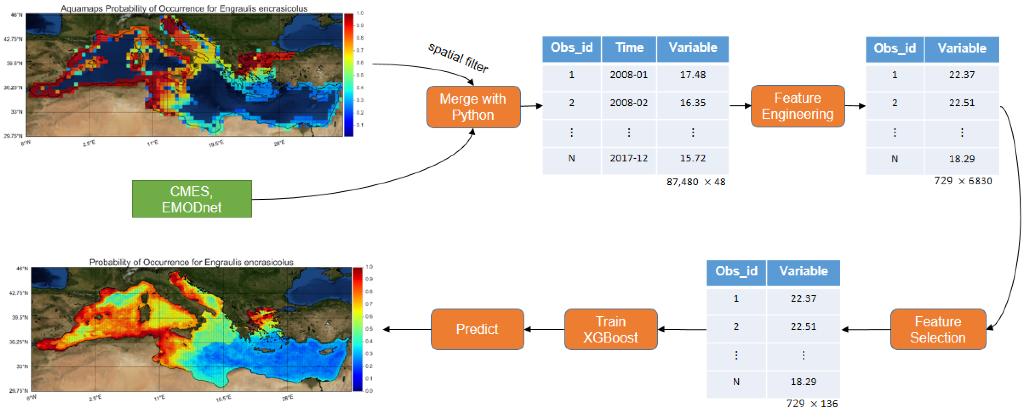
More specifically, the herein developed model was trained with roughly $\times 3.5$ times more observations than the average related work (improvement over observations). With the use of feature engineering, 6830 features were extracted and subsequently, feature selection was performed, leading to the selection of the most important ones (improvement over features and collinearity). Finally, a machine learning algorithm that has never been applied in previous SDM literature, namely, XGBoost [32] was used. XGBoost offers regularization preventing the model from overfitting, it can handle missing values and it provides the optimum number of boosting iterations in a single run, minimizing the time needed for its performance. Instead of using presence-absence data for binary classification, like most studies do, the problem was transformed to a regression one (improving the unbalance of presence-absence datasets) and predict the probability of occurrence based on data provided by the AquaMaps database. Furthermore, fish species distributions were interrelated to oceanographic and environmental conditions, utilizing the high resolution Copernicus Marine Environmental Service (CMEMS) products [33] and the European Marine Observation and Data Network (EMODnet) [34] databases for the whole Mediterranean Sea. The best feature categories and environmental predictors for each species and overall were analyzed. Finally, with the use of the trained SDM, AquaMaps spatial resolution was improved ($\times 8$ higher) and high resolution maps (0.0625 arc-minutes) without any spatial gaps were constructed, covering the whole Mediterranean Sea, for the eight commercial pelagic fish species.

2. Materials and Methods

2.1. Study Area

All species observations and environmental variables are situated in the Mediterranean Sea. With regard to environmental conditions, Mediterranean Sea exhibits a unique structure as evaporation exceeds river flux and precipitation, leading to the intrusion of Atlantic water masses. The limited river discharge makes the Sea predominantly oligotrophic to ultra oligotrophic. Salinity decreases from east to west; temperature decreases from north-west to south-east; thermal boundaries in deep waters are absent [35], and areas near the coast are affected locally by human activities [36]. The current oceanographic, environmental, and climatic challenges of the Med, together with the presently operating Observing and Forecasting Systems and existing platforms which offer downstreaming services for users and stakeholders, are extensively reviewed by Tintoré et al. [37]. According to Reference [38] there are approximately 17,000 marine species occurring in the Mediterranean Sea, while AquaMaps [39] provides distribution ranges for 1971 fish species and invertebrates.

2.2. Species Data

In this study, eight commercial fish species were chosen for analysis and prediction. This selection was based on the following criteria: (i) these species represent the most common commercial fish in the Mediterranean Sea, occurring in a plethora of locations, (ii) they are pelagic species living in different depth ranges, and (iii) they demonstrate a variety of preferred environmental conditions, especially at the upper parts of the water column. It is a challenging task to create a single generic model that performs the best for all species. Most of these pelagic fish species are small and medium-sized, and the depth range of each appears in

Table 1. Species of the present study and number of observations.

Scientific Name	Common Name	Depth	Samples
E. encrasicolus	European anchovy	0–400	729
S. pilchardus	European pilchard	10–100	596
S. aurita	Round sardinella	0–80	720
S. colias	Atlantic chub mackerel	0–300	676
S. scombrus	Atlantic mackerel	0–1000	807
S. smaris	Picarel	15–328	1225
T. thynnus	Bluefin tuna	0–1000	1237
X. gladius	Swordfish	0–3000	1230

: European anchovy (Engraulis encrasicolus), European pilchard or sardine (Sardina pilchardus), round sardinella (Sardinella aurita), Atlantic chub mackerel (Scomber colias), Atlantic mackerel (Scomber scombrus), picarel (Spicara smaris), Atlantic bluefin tuna (Thunnus thynnus) and Swordfish (Xiphias gladius).

Anchovy is a summer spawning (April to September in the Mediterranean), fast growing, short living, and early maturing small pelagic fish [40,41]. It is a low trophic level planktivorous species with preference for warm water temperatures [9]. Together with sardine, they constitute around 40% of the total marine fishery landings in the Mediterranean, a percentage that fluctuates depending on the country and which is highest along the northern Mediterranean coastline [9].

Sardine is a winter spawning (October to March in the Mediterranean), fast growing, and early maturing small pelagic fish with a short lifespan [41] that primarily feeds on zooplankton and is preyed upon by large pelagic fish, marine mammals, and seabirds. It generally prefers low water temperatures and constitutes around 20% of the marine fishery landings in the Mediterranean Sea, especially along the northern coastline [9]. Sardine and anchovy alternate in high abundances and landings [42].

Round sardinella is also a fast growing and early maturing small pelagic fish with short lifespan, which spawns over a narrower (May to July in the Mediterranean Sea) time period [43]. It feeds mainly on zooplankton [44] and has a strong preference for warm waters [9]. Although its abundance is increasing across the Mediterranean Sea as a result of sea warming (western Mediterranean: [45]; eastern Mediterranean: [46]), round sardinella’s contribution to marine fishery landings is confined to the southern Mediterranean coastline.

Atlantic chub mackerel is a medium sized pelagic fish, which spawns over late-spring/early -summer months (May to June) in the Mediterranean Sea [47]. Its growth rate is medium and its lifespan is around 7 years [48]. It is a high trophic level species as it feeds on fish and zooplankton [48] and prefers warm waters [9]. Atlantic chub mackerel is a commercial species in many Mediterranean countries.

Atlantic mackerel is a medium sized pelagic fish, which spawns during winter (December to March) in the Mediterranean Sea [47]. It grows at a medium rate and may reach 17 years of age [48]. It is positioned high in the food web and prefers cold waters [9]. Similar to chub mackerel, Atlantic mackerel is a commercial species in most Mediterranean countries.

Picarel is a small-sized hermaphroditic spring spawning species (April to May), which spawns on sandy bottoms where nests are excavated [49]. It grows fast, has a short lifespan, generally prefers cold water temperature, and is positioned low in the food web [48]. In some countries of the Mediterranean, picarel contributes to the total landings.

Bluefin tuna is a highly migratory large pelagic fish with a very high commercial value. Its eastern Atlantic population spawns in the Mediterranean Sea [50] at the age of 3 years and at a size exceeding 100 cm [51]. Its stock, which is subject to dynamic management with a total allowable catch (TAC) allocated each year, collapsed in the late 2000s [52] but appears to be recovering after drastic decrease of TAC.

Swordfish is also a highly migratory large pelagic fish with a very high commercial value, which spawns in the eastern Mediterranean Sea [53] in May and June [54]. Its stock is subject to dynamic management with a total allowable catch (TAC) allocated each year.

Species probability of occurrence data were retrieved from AquaMaps. AquaMaps utilizes large sets of occurrence data (Figure 1), derived from a mixture of online, freely available collection databases (such as GBIF and OBIS), independent knowledge on species distribution, and fishery habitats (from FishBase). These occurrence data points are combined to species-specific envelopes of environmental preferences, such as minimum, mean and maximum depth, depth standard deviation, distance from land, ocean area, annual mean ice concentration, annual mean primary production, annual minimum, mean and maximum sea surface temperature, sea surface temperature standard deviation, sea surface temperature range, annual mean sea bottom temperature, annual minimum, mean and maximum salinity, and annual mean bottom salinity, to determine the suitability of a given area in the ocean for a particular species [55]. Predictions of relative probabilities of species occurrence are provided by AquaMaps, illustrated as color-coded species range maps in a global grid of half-degree latitude and longitude cell dimensions. AquaMaps predictions have been validated using independent and effort-corrected survey data [56].

AquaMaps was based on global, coarse environmental databases (e.g., NCEP, World Ocean Atlas, World Ocean Atlas Bottom Source Information, SeaAroundUs and more), and as a result the relative “probability of occurrence” per species is also coarse. Thus, in this work all Meditterranean Sea-filtered locality records, each with probability of occurrence, were collected from the expert-reviewed AquaMaps datasets. These datasets were the latest available (2016 and later), and were referring to the same time-frames as the environmental variables selected in Section 2.3. These initial datasets include gridded coordinates, as well as the overall probability of the species existing in that location. In contrast to other related works [17,18,22,23], the datasets used in this study include a larger number of observations, ranging from 596 for sardine to 1237 for bluefin tuna.

2.3. Environmental Variables

Species Distribution Modelling involves the merging of species occurrence data with environmental layers collected from other sources. Each longitude–latitude occurrence pair must be matched with the environmental conditions taking place in that exact or closest location. Environmental variables are known in the bibliography with various names such as variables, parameters, indicators, predictors, and features. In order to choose the most appropriate parameters, a domain knowledge from experts is needed, and depending on the individual problem to solve, researchers select the most appropriate set of variables for their experiments. Each environmental problem is unique and requires to be treated differently in terms of parameter selection. However, some variables are extensively used in most related works, such as sea surface temperature, salinity, bathymetry, and distance to coast. In this work, fifteen initial predictors were selected based on the variables that have been reported to affect fish distribution. The use of these particular environmental variables is based on data availability and ecological degree of relevance for fish species.

There are several online resources that give access to marine environmental variables. Most species distribution models use low resolutions for their models. Having high resolution, spatially explicit, continuous data is rare in marine environments [21]. However, for the Mediterranean Sea there are two platforms that provide high resolution envelopes for environmental predictors describing marine conditions. These are the Copernicus Marine Environmental Service (CMEMS) database [33], which was used for the extraction of variables changing in time, and the European Marine Observation and Data Network (EMODnet) [34], which was used for the bathymetry and substrate datasets.

Variables chosen for this work are divided into two categories, temporal and static. The temporal include temperature, salinity, dissolved oxygen, meridional current, zonal current, chlorophyll-$\alpha$, euphotic depth, secchi disk depth, wave height, nitrate, and phosphate. Static include distance to coast, distance to major river mouths, bathymetry, and substrate. Temporal variables are extended into time and vertical space. In particular, monthly-mean data with a timespan of 10 years, from January 2008 to December 2017 were collected resulting in 120 values for each variable at each location. Also, because the selected species are pelagic, 2 depth levels were considered. These include values for sea surface and 100 to 300 m mean.

Table 2. Environmental variables. * These three spatial resolutions are in kilometers ($1\times 1$, $4\times 4$, and $4\times 4$ km, respectively), and they are converted in arc-minutes for comparability; one arc-degree at the Mediterranean is roughly 111 km.

Variable	Depths	Spatial Resolution	Data Product	Data Type	Data Provider
Temperature (${}^{\circ }$C)	2	0.0625${}^{\circ }$ × 0.0625${}^{\circ }$	MEDSEA_REANALYSIS _PHYS_006_004	Sea Physics Reanalysis	CMEMS
Salinity (psu)	2	0.0625${}^{\circ }$ × 0.0625${}^{\circ }$	MEDSEA_REANALYSIS _PHYS_006_004	Sea Physics Reanalysis	CMEMS
Diss. Oxygen (mmol/m${}^3$)	2	0.06${}^{\circ }$ × 0.06${}^{\circ }$	MEDSEA_REANALYSIS _BIO_006_008	Biogeochemistry Reanalysis	CMEMS
Meridional Current (m/s)	2	0.0625${}^{\circ }$ × 0.0625${}^{\circ }$	MEDSEA_REANALYSIS _PHYS_006_004	Sea Physics Reanalysis	CMEMS
Zonal Current (m/s)	2	0.0625${}^{\circ }$ × 0.0625${}^{\circ }$	MEDSEA_REANALYSIS _PHYS_006_004	Sea Physics Reanalysis	CMEMS
Chlorophyll-$\alpha$ (mg/m${}^3$)	1	0.009${}^{\circ }$ × 0.009${}^{\circ }$ *	MEDSEA_REANALYSIS _BIO_006_008	Biogeochemistry Reanalysis	CMEMS
Euphotic Depth (m)	1	0.036${}^{\circ }$ × 0.036${}^{\circ }$ *	EMIS—MERIS Monthly climatology Surface productive layer	Satellite	EMIS-MERIS
Secchi Disk Depth (m)	1	0.036${}^{\circ }$ × 0.036${}^{\circ }$ *	OCEANCOLOUR_GLO _OPTICS_L4_REP _OBSERVATIONS_009_081	Satellite Observations	CMEMS
Wave Height (m)	1	0.042${}^{\circ }$ × 0.042${}^{\circ }$	MEDSEA_HINDCAST _WAV_006_012	Seas Waves Hindcast	CMEMS
Nitrate (mmol/m${}^3$)	2	0.06${}^{\circ }$ × 0.06${}^{\circ }$	MEDSEA_REANALYSIS _BIO_006_008	Biogeochemistry Reanalysis	CMEMS
Phosphate (mmol/m${}^3$)	2	0.06${}^{\circ }$× 0.06${}^{\circ }$	MEDSEA_REANALYSIS _BIO_006_008	Biogeochemistry Reanalysis	CMEMS
Dist. to Coast (km)	–	–	–	–	GIS
Dist. to Major River (km)	–	–	–	–	GIS
Bathymetry (m)	–	0.0625${}^{\circ }$× 0.0625${}^{\circ }$	EMODnet DTM for Regional Seas	Digital Terrain Model	EMODnet
Substrate	–	–	EMODnet Seabed substate product	Seabed substrate 1:1M	EMODnet

summarizes the environmental variables used. More information about such variables can be found in Reference [27].

2.4. Models and Evaluation

A number of machine learning models and feature selection techniques were used in this work. First of all, 10 regression algorithms were tested during the initial experiments, both linear and non-linear, in order to pick the overall best performing one among species. The algorithms used are the following: Linear Regression (LR), Least Angle Regression with Lasso (LARS), Support Vector Machine Regression (SVR), Decision Tree (DT), Random Forest (RF), Extremely Randomized Trees (ET), Adaptive Boosting (AdaBoost), Gradient Boosting (GBM), Extremely Gradient Boosting (XGBoost) and Light Gradient Boosting (LightGBM). 5 feature selection techniques and an ensemble one were used to rank the features according to their importance in determining pelagic fish species distribution over the Med. The goal of feature selection was to eliminate irrelevant and noisy features, by keeping the ones that can predict the target best. This technique decreases the computational time, improves the performance of the algorithm, avoids over-fitting, and creates better general models.

There are three types of feature selection methods: filters, wrappers, and embedders. Filters are used before machine learning, and they rank the features based on their intrinsic properties, like variance and correlation. Wrappers use a machine learning algorithm as a black box evaluator to rank the features. Embedded methods combine filters and wrappers by first computing statistical measurements on the data and then using an algorithm. We used two filters, Mutual Information and Fisher Score, one wrapper namely SHAP and two embedders using Random Forest and XGBoost. The ensemble technique followed is called Reciprocal Ranking and computes the final rank $r\left(f\right)$ of a feature f as follows:

$$r\left(f\right)=\frac{1}{{\sum }_j^{}\frac{1}{r_j\left(f\right)}},$$

where $j=1,2,\dots ,N$ are the feature selection methods, and $r_j\left(f\right)$ is the rank of the feature according to the jth method.

We split the datasets in train (80%) and test (20%) set. For training and validation we used 10-fold cross validation. Validating a model with cross validation reduces the danger of over-fitting and results in a better general model that can have high performance on an unknown dataset. Root mean square error (RMSE), representing the mean standard deviation of prediction errors, was chosen as the metric for all experiments, since the target is a continuous variable.

3. Results

This section describes all the actions taken for the completion of this work. Figure 2 serves as a graphical abstract of the whole process. It shows the collection of data from AquaMaps and the merging with the environmental envelopes, the creation of the panel dataset, its transformation with feature engineering to the final dataset, the selection of the top variables, and the prediction with XGBoost on the whole Mediterranean Sea with high resolution.

3.1. Dataset Creation

Several steps were taken to create the dataset. Firstly, the AquaMaps website was accessed to download the initial data for each species. These data include the coordinates of the observation and the probability of occurrence in that location. A spatial filter was applied to remove all points outside the Mediterranean Sea. Having the locations, third party datasets that provide environmental variables were merged with the probability of occurrence data. The environmental variables can be seen in Table 2 and the publicly available sources that give access to them are CMEMS and EMODnet. The predictors include the coordinates and the values of the measured variable. A Python code was developed to compare the coordinates between the initial dataset and each environmental variable in order to find the point with the nearest distance. That point’s value was added to the new dataset. Also, as CMEMS provides water column data and the studied species are pelagic, for each predictor, the mean from 100 to 300 m depth per parameter was also computed as extra feature to test its strength. The output of this procedure was the full dataset, with the species’ coordinates, the probability of occurrence reported in AquaMaps, and the environmental variables describing each observation from third party datasets.

Another important part of this work is that variables were not limited in only a single value per observation, but instead temporal data were also considered. In particular, monthly values for a period of 10 years from 2008 to 2017 were extracted, resulting in 120 values per observation. This data format is called panel data and includes several rows in the dataset for each observation. It is not possible to perform machine learning in such data, because each observation should have a unique row to train. Thus, the next step is to transform this panel dataset into the final dataset for machine learning.

3.2. Feature Engineering

Feature engineering is the process of creating new features from the existing ones. Some of these features might prove very efficient for the regression algorithm and can help the prediction of the target variable. Since time series data were considered, a very large number of features was created. These features include descriptive statistics like mean, median, standard deviation, maximum, minimum, maximum to minimum difference, skewness, kyrtosis, mean absolute deviation, and several quantiles. All of them were computed at annual and monthly basis. For example, a feature can be ‘temperatureSurface_April_mean’. Time series and signal related features were also computed, like moving and expanding averages, maximums, minimums, medians, quantiles, skewness, mean change rate, short and long term averages, Hilbert transformation, Hann window, spline interpolation, Gaussian spline interpolation, trend, median-filtered mean, Wiener-filtered mean, Savitzky-Golay mean, downsample, detrend, relative minima and maxima, local minima and maxima and features that take into account spatial neighbors of each observation.

The above-described feature engineering procedure created a total of 6830 features. This is a huge number compared to the number of observations (≈902 on average). Having seven times more features than samples can cause overfitting and it is computationally inefficient. Thus, the next vital step is to perform feature selection to get the feature importance and select the very top performing ones. The reason for creating so many features is because it is impossible to know a priori which features are the best, and to have a diversity in the feature selection process. But before proceeding to feature selection, a machine learning algorithm has to be chosen.

As stated in Section 2.4, ten regression algorithms were compared using all features (6830) in the test set. The test set is consisted of randomly picked areas from the dataset (20% of initial dataset). The Python language was used, along with the libraries scikit-learn, xgboost and lightgbm. The parameters of the algorithms were left to their default values. This is the baseline experiment and its outcome is shown in

Table 3. Algorithm comparison using RMSE of the 20% test set of locations using all the features as predictors for baseline selection per species.

	XGBoost	GBM	LGBM	ET	RF	AdaBoost	DT	LARS	SVR	LR
Engraulis encrasicolus	0.2369	0.2403	0.2359	0.2439	0.2495	0.2432	0.2784	0.3527	0.3491	0.3724
Sardina pilchardus	0.1807	0.1820	0.1889	0.1872	0.1978	0.1916	0.2621	0.3510	0.3488	0.3670
Sardinella aurita	0.2548	0.2557	0.2484	0.2506	0.2482	0.2587	0.3283	0.3460	0.3432	0.3528
Scomber colias	0.1783	0.1758	0.1795	0.1895	0.1772	0.1924	0.2377	0.2448	0.2422	0.2662
Scomber scombrus	0.1254	0.1276	0.1365	0.1317	0.1376	0.1351	0.1694	0.2158	0.2164	0.2191
Spicara smaris	0.1221	0.1283	0.1267	0.1258	0.1201	0.1427	0.1670	0.1378	0.1649	0.1816
Thunnus thynnus	0.0862	0.0868	0.0875	0.0916	0.0913	0.0969	0.1160	0.2322	0.2305	0.2397
Xiphias gladius	0.0794	0.0781	0.0766	0.0805	0.0823	0.0879	0.1127	0.2228	0.2209	0.2227
Mean Score	0.1579	0.1593	0.1600	0.1626	0.1630	0.1685	0.2089	0.2628	0.2645	0.2776

. The overall best algorithm among species is the XGBoost and is the one that will be used for the rest of the paper. From these results we can observe that the boosting models perform similarly best, while simpler models like Decision Tree and the linear models have the lowest performance. Species Distribution Modeling data seem to favor nonlinear models. Nonlinear regression is much more flexible in the shapes of the curves that it can fit and this kind of data cannot be easily modeled with simple linear models. Based on the above results, the XGBoost, Gradient Boosting or LightGBM are recommended for similar problems.

3.3. Feature Selection

The goal of feature selection is to rank the features according to their importance. First, we used five selection algorithms for this purpose and ensembled their rankings using Reciprocal Rank as stated in Section 2.4. The ranking of the latter is usually superior of the individual ones, and is the one that was used in this work. The reason of its success is firstly that it takes as inputs rankings of diverse feature selection techniques, where the disadvantages of one might be compensated by another, and secondly that it is a harmonic mean formula. This means that if one of the five algorithms ranks a feature among the top and the other four rank it lower, then it will remain in a high position on the final ensemble ranking since the harmonic mean is biased towards the smaller of the numbers.

Figure 3 gives a graphical insight of the exceptional strength of feature selection and the boost that it offers to the regression problem. It is a backward stepwise selection process, starting with all the features and eliminating them according to their rank of diminishing importance. All runs used 10-fold cross validation for training and evaluation of the model using XGBoost. A clear pattern to each species seems present. Using the baseline of all features (leftmost side of plots), the Root Mean Square Error is relatively high and stays there up to around 70% of features removed (0.3 feature cutoff). From that point it decreases, until it reaches its lowest value at a percentage of around 2% features retained (i.e., around 136 features). The 2% percentage slightly varies between species (from 1.5% to 2.5%), but as a general model is constructed, the, 2% cutoff will be used. If even less features are used, then performance drops (RMSE increases again, drastically). This behavior is similar for all species, regardless of the actual RMSE values, which vary depending on the species. A reason for this outcome is that all datasets were created in a similar manner. The feature engineering procedure created the same features for each species. This does not mean that the top 2% of them are the same. Each species, varies on the predictors that are affecting its distribution.

The baseline runs for all species using the XGBoost algorithm are improved, as it can be seen in

Table 4. XGBoost performance of each species. Baseline is the RMSE score of the test set before feature selection. Validation is the 10-fold cross validation RMSE using the top 2% features. Test is the RMSE score of the test set using the top 2% of features. Improvement is the test’s improvement over baseline.

		Validation	Test
Species	Baseline	2% Feats	2% Feats	Improvement
E. encrasicolus	0.2369	0.2075	0.1503	36.5%
S. pilchardus	0.1807	0.1562	0.1287	28.8%
S. aurita	0.2548	0.2218	0.1877	26.3%
S. colias	0.1783	0.1596	0.1302	26.9%
S. scombrus	0.1254	0.1152	0.0738	41.1%
S. smaris	0.1221	0.1153	0.0869	28.8%
T. thynnus	0.0862	0.0812	0.0471	15.3%
X. gladius	0.0794	0.0730	0.0464	41.5%

, from 26.3% for aurita to even 45.5% for thynnus. The average performance boost for the eight species is about 34% on the test set. As it can be seen with this evaluation, the results on the validation and the test set are similar, indicating lack of overfitting.

As a final step in the modeling procedure, the initial classifiers from Section 3.2 are again deployed, this time using the top features as defined by the process of feature selection. The test set is the same as before (20%), when XGBoost was used. The results are available on

Table 5. Test set performance of the algorithms used in Section 3.2. The baseline is when the model using all features and 2% feats is when the model uses the top 2% of the features.

	GBM		LGB		ET		RF
Species	Baseline	2% Feats	Baseline	2% Feats	Baseline	2% Feats	Baseline	2% Feats
E. encrasicolus	0.2403	0.1420	0.2359	0.1445	0.2439	0.2452	0.2495	0.1398
S. pilchardus	0.1820	0.1374	0.1889	0.1306	0.1872	0.1930	0.1978	0.1318
S. aurita	0.2557	0.1905	0.2484	0.1917	0.2506	0.2844	0.2482	0.1842
S. colias	0.1758	0.1188	0.1795	0.1267	0.1895	0.1655	0.1772	0.1356
S. scombrus	0.1267	0.0736	0.1365	0.0775	0.1317	0.1111	0.1376	0.0744
S. smaris	0.1283	0.0984	0.1267	0.0961	0.1258	0.1484	0.1201	0.0870
T. thynnus	0.0868	0.0446	0.0875	0.0465	0.0916	0.0850	0.0913	0.0508
. gladius	0.0781	0.0462	0.0766	0.0467	0.0805	0.0870	0.0823	0.0503

and

Table 6. Test set performance of the algorithms used in Section 3.2. (continued from Table 5).

	ADA		DT		SVR		LR
Species	Baseline	2% Feats	Baseline	2% Feats	Baseline	2% Feats	Baseline	2% Feats
E. encrasicolus	0.2432	0.1710	0.2784	0.2318	0.3490	0.3446	0.3724	0.1962
S. pilchardus	0.1916	0.1542	0.2621	0.1551	0.3488	0.2552	0.3670	0.1904
S. aurita	0.2587	0.1995	0.3283	0.2484	0.3432	0.3589	0.3528	0.3720
S. colias	0.1924	0.1427	0.2377	0.1729	0.2420	0.2585	0.2662	0.1604
S. scombrus	0.1351	0.1002	0.1694	0.1139	0.2164	0.1756	0.2191	0.1026
S. smaris	0.1427	0.1153	0.1670	0.1165	0.1649	0.1377	0.1816	0.1208
T. thynnus	0.0969	0.0611	0.116	0.0678	0.2305	0.1130	0.2397	0.0873
X. gladius	0.0879	0.0596	0.1127	0.0647	0.2209	0.1203	0.2227	0.0978

. It is clear that feature selection improves all algorithms except Extra Trees Regression (improvement in only 3 species), Support Vector Regression (improvement in 6 species), and Linear Regression (improvement in 7 species). The improvement in all algorithms was of a considerable degree. Some of them had an exceptional increase in performance, like Linear Regression (42% improvement over baseline). The best models are again the same as in the initial comparison. These are XGBoost, Gradient Boosting and LightGBM, with XGBoost performing again slightly better on average. The results indicate that the ensemble feature selection used in this work is a consistent method, that improves almost all algorithms and by a high margin. Finally, a model has to be chosen to predict the probability of occurrence of each species in the whole Mediterranean, and that model will be XGBoost.

3.4. Feature and Predictor Importance

Having the model trained and all features ranked with Reciprocal Ranking, valuable information about which features are meaningful for such problems can be extracted. Moreover, the variable that refers to a predictor may be derived using a mathematical formula. For example, ‘temperature Surface April mean’ is a feature that refers to the predictor ‘temperature’. Our feature engineering procedure constructed various features for each predictor. The herein produced features belong to several categories. As an example, the aforementioned feature belongs to the categories ‘mean’, ‘month’, and ‘surface.’

It is difficult to know a priori which categories perform better, so through feature engineering all possible features were created, knowing that feature selection will be able to select the top ones. However, after the experiment an importance analysis for each feature category may be performed, based on its Reciprocal Ranking score. In order to do this, all features that fall within each category were collected, and a descriptive statistic was calculated. One option for this statistic would be their mean score. However, the mean is prone to outliers and is not representative. Another option would be to pick the single best (minimum score) feature for each category. This is also not a good choice, because some feature categories might have more features than others. So, the 2% quantile was selected as the most appropriate descriptive statistic to extract a metric for the overall performance of each category. The 2% quantile is compatible with the best model which uses the top 2% of features. The feature relative strength analysis is depicted in Figure 4. Lower numbers have greener colors and represent the feature categories with the lower 2% quantile of Reciprocal Ranking. In addition, Figure 5 depicts the strengths of the top-10 predictors for each species.

3.5. Improving Aquamap’s Resolution And Coverage

After feature selection, our data are ready to be fitted in the XGBoost model. For each species, the data fitted consisted of all the observations (train + test) and the top 136 features. A prediction/projection dataset was prepared with $67,000$ points covering the whole Mediterranean Sea. The resolution of this dataset is 0.0625${}^{\circ }$× 0.0625${}^{\circ }$, as it is the lowest available resolution from our data sources (CMEMS, EMODnet). For all these coordinates, the environmental variables were extracted in the same manner as the in training datasets. Finally, the probability of occurrence for each species in this dataset was predicted. The results can be seen in Figure 6. Through the above described machine learning process, we managed to create a single generic model and produce high resolution maps covering the whole Mediterranean basin for the eight most commercial pelagic fish species.

4. Discussion

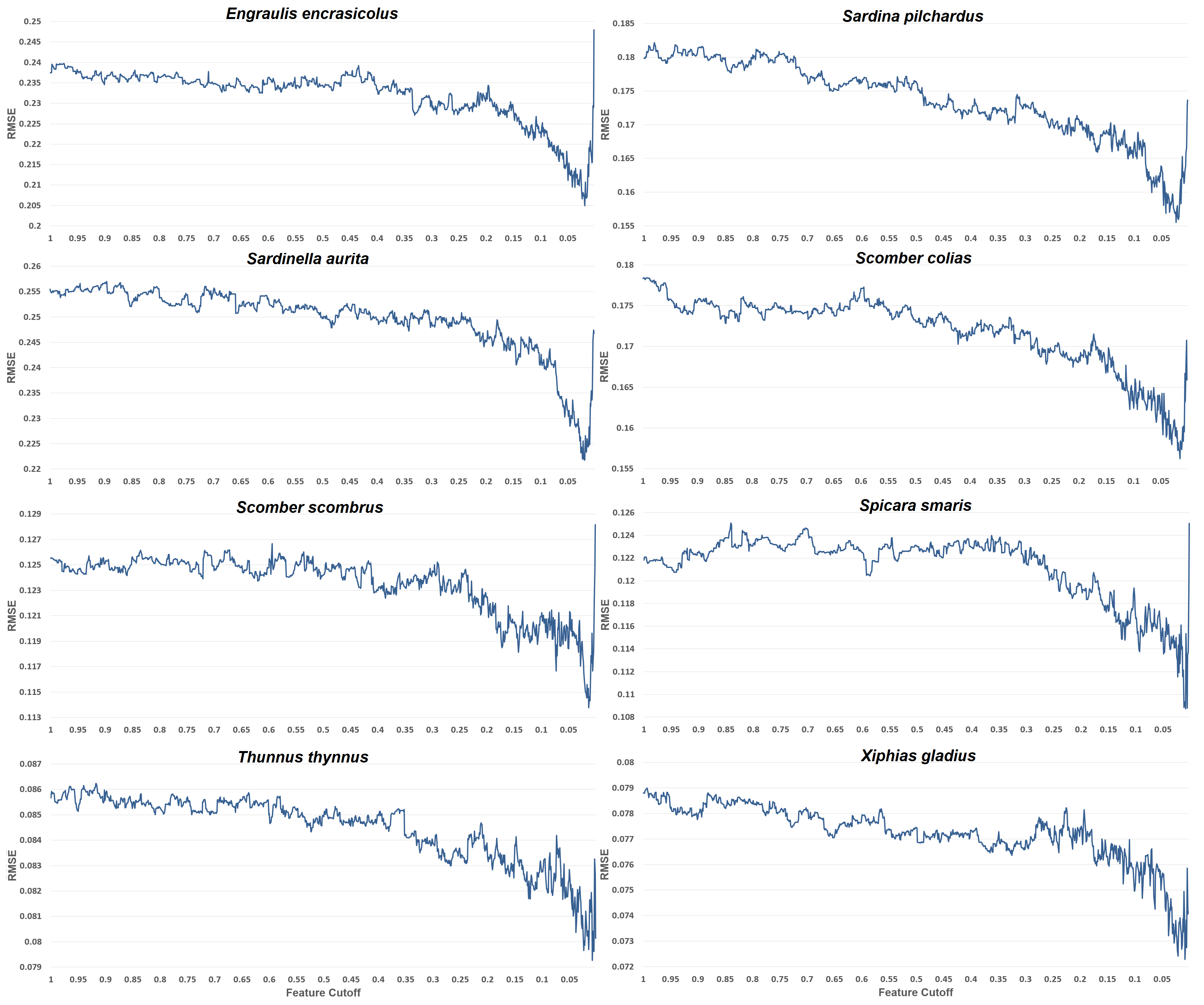
Understanding the environmental processes influencing fish species abundance is important in order to manage the fishing grounds and offer advice on the exploitation of this important resource. It is evident that out of the 6830 features that our feature engineering process generated, about 136 (or 2%) of these are the most important and are advised to be used to reach the lowest possible prediction error. Most of the other species distribution studies, use about 5 to 20 features for their models, which are an order fewer than the 136 used in the present model. This happens because (a) very few studies (if any of them) use time series features, (b) they do not generate such a huge number of features to choose from, (c) they empirically pick the features depending on their domain knowledge and data availability. The present approach is different from the existing studies in this respect. It is not limited to basic features like maximum sea surface temperature or mean salinity, but it expands upon very detailed time series features. It suggests that about 2% of such features are appropriate for all our datasets, and if less predictors are used, then performance worsens. For overfitting and generalization purposes the exact number of features that minimizes their RMSE for each species is not used, but rather a better bias-variance trade-off feature cutoff is preferred.

Having very few features, the model’s reliability diminishes, since these features are very specialized, and case only the very top-ranked ones are kept, whole predictors like chlorophyll or nitrate cease to exist in the model. Thus, having only variations of temperature is not enough. The whole feature selection process not only boosts execution time and performance, but also gives valuable insights into which variables are most important for each species. These insights are depicted in Figure 4, where the importance of feature categories generated by the feature engineering process is visible.

The figure clearly shows which feature categories are worth investing time in feature engineering and which are not. The neighbor-based features seem to be the strongest ones. This is the only hand-crafted feature and it computes the minimum, mean, maximum and standard deviation of the eight cells that surround the given one on all predictors. For example, the feature ‘temperatureSurface_neighbor_mean’ calculates for every observation the mean surface temperature of its eight neighboring observations. Surrounding cells have been mentioned before [28] that might influence the distribution of species. It is evident that the probability of species presence is greatly affected by the conditions of the neighboring environmental parameters. This means that the species live in large areas next to each other and not in small isolated ones with different conditions. The importance of neighboring features comes in agreement with the fact that longitude and latitude predictors are also vital as it will be demonstrated later on. In the same manner, features with extreme values depict strong importance. Minima, maxima and quantiles are much stronger in terms of importance than means and medians. These results are in line with the bibliography, as the authors of Reference [57] state that quantiles near the maximum create good features when other variables are not limiting, and Reference [58] claims that low quantiles are relevant to estimate the lowest recruitment level for a species. Another feature of descriptive statistics, which is of major importance is skewness.

It is very common for researchers to use mean-monthly data [16,59] and only rarely mean-annual data. In this study, it was demonstrated that both feature categories are strong, with the monthly features being slightly better. This happens because some stages in fish life, such as breeding and migration, occur in certain months. By comparing the surface values to the mean of 100 to 300 m, it becomes clear that the latter falls behind. Conditions found below the surface are rarely accurately known [60], thus it is advised to use surface values. All feature categories from the signal processing area related to filters are the worst performing ones. The mean expanding (exponential window) and classical sta-lta (Short Time Average over Long Time Average), which is used in seismic events, obtained very high importance. One would expect that relative minima and maxima and peaks would be good feature categories, like the minimums and maximums of the descriptive statistics. This is not true, as all the temporal environmental variables have high seasonality and the peaks are insignificant.

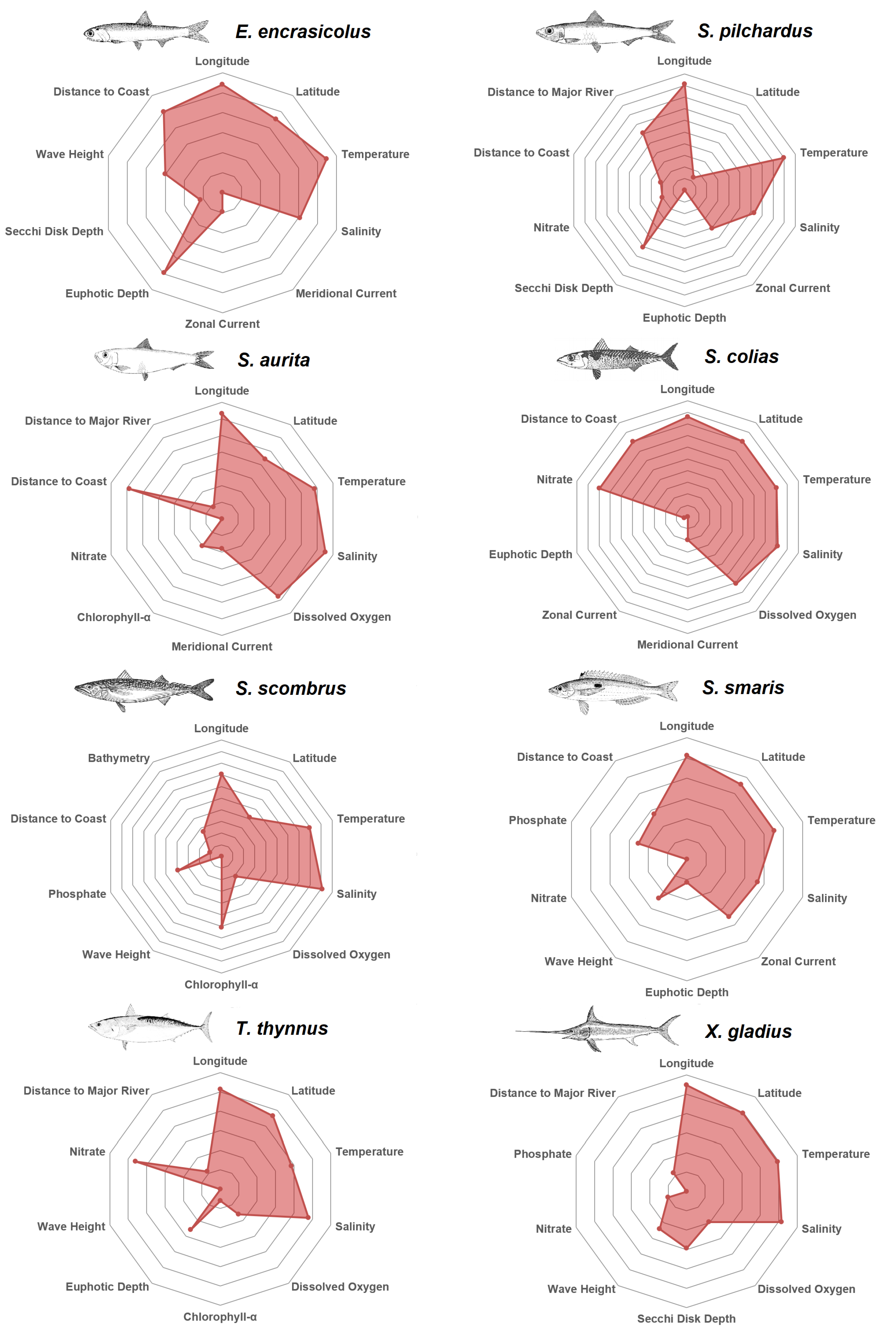
After having investigated the features and their respective predictors that were considered as most valuable by the Reciprocal Ranking technique, in Figure 5 the top 10 predictors for each species are depicted in alphabetical order. The plots are qualitative and normalized so that the 10th predictor would be at the center of the plot. Every decagon represents one unit in terms of Reciprocal Ranking importance. For example, anchovy zonal current is five times less important than distance from the coast. Longitude is among the top predictors for every species, in agreement with the western-to-eastern gradient in the trophic conditions of the Mediterranean Sea. This longitudinal gradient represents changes in water temperature, chlorophyll concentration and mixed layer depth over the epipelagic layer [61]. The Anchovy is mostly affected by the distance from the coast, the temperature and the euphotic depth; pilchard by water temperature, salinity, secchi disk depth and distance from the major rivers; round sardinella by salinity, temperature, distance from the coast and dissolved oxygen; atlantic chub mackerel by salinity, temperature, latitude, nitrate and distance to from the coast; atlantic mackerel by salinity, temperature and chlorophyll-$\alpha$; picarel by temperature, zonal current, salinity and latitude; bluefin tuna by salinity, nitrate and latitude, and swordfish by salinity, temperature and latitude.

Because of their fast life history strategy (rapid growth, early maturation, short lifespan), small pelagic fishes and especially their recruitment success [10], hence their distribution, abundance and fishery catches, are vulnerable to climate and environmental forcing [12,13,42]. However, the decline in landings of most small and medium pelagic species is only partially attributed to climate and environmental factors because, especially in the Mediterranean Sea, over-exploitation still remains the main driving force of their populations [9,62]. Indeed, overfishing has been reported to modify the abundance, composition, and distribution of pelagic species, but also to induce drastic changes of state [63].

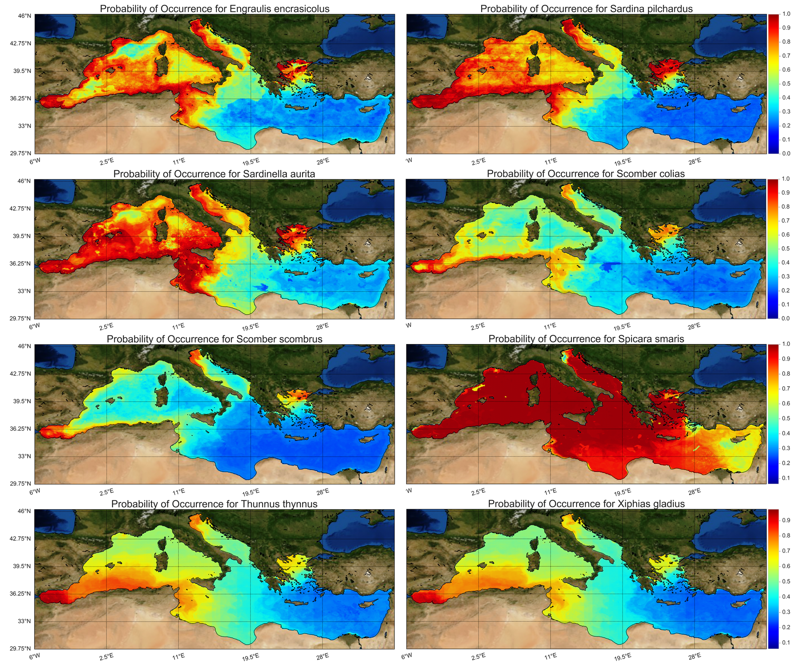
Following the above-described west-to-east gradient, the probability of occurrence of small pelagic fishes was higher in the western Mediterranean Sea and declined eastwards (Figure 6) with the exception of picarel, which was abundant throughout the basin. For medium and large-sized pelagic fishes, the probability of occurrence was higher in certain areas of the western and northern Mediterranean, while they were completely absent from the southeastern part of the basin, as a results of the raised temperature and salinity and the low chlorophyll levels at the surface layer (Figure 6). Small and medium pelagic species are generally concentrated in areas of high productivity because most of them are mainly plankton feeders [64]. These areas are associated with cooler and fresher nutrient rich water masses that could be either upwelling areas (e.g., west African coast: [63]), coastal areas affected by riverine input (e.g. NW Mediterranean: [65]) or areas affected by both riverine input and other water masses (e.g. Black Sea Water influx in the northern Aegean Sea: [66]). These conditions are typical for the northern Mediterranean coastline and create a northwestern-to-southeastern gradient in productivity. Indeed, biological productivity in the Mediterranean basin has been reported to decrease from north to south and from west to east and it is inversely related to the increase in temperature and salinity [67] indicating that the Mediterranean Sea is highly heterogeneous between its basins [68]. This gradient makes longitude appear vital in the distribution of pelagic species and even latitude seems significant, despite the narrow latitudinal axis of the Mediterranean due to riverine input that mostly affects the northern coastline. Changes in primary productivity, the composition of plankton community and the abundance of key plankton species, that may be climate-driven [69], directly affect the distribution of small pelagic fishes, which preferentially feed on zooplankton, such us anchovy and sardine [70], but they could also indirectly affect their somatic condition [10]. Enhanced primary and secondary productivity benefits these planktivorous species by increasing the availability of their prey (bottom-up control), but at the same time improves their somatic condition [71]. Although NW Mediterranean is richer in pelagic fishes, sharp regional gradients and gaps in the probability of occurrence exist, mostly in anchovy and round sardinella distribution (Figure 6a,c). Strong currents and meso-scale eddies in Alboran Sea, the Tyrrhenian Current and the Liguro-Provençal Current favor the presence of these species. In the Gulf of Lions the freshwater impact of Rhone River and the up- and downwelling events explain the sharp differences in fish species occurrence.

According to the findings of the present work (Figure 5,

Table 7. Overall predictor importance among the eight commercial fish species ranked by Friedman Rank.

Predictor	Friedman Rank
Longitude	1.5
Salinity	2.625
Temperature	3
Latitude	4.625
Distance to Coast	7.25
Dissolved Oxygen	8.875
Nitrate	9.375
Zonal Current	9.75
Euphotic Depth	10
Wave Height	10
Phosphate	10.25
Chlorophyll-$\alpha$	10.375
Secchi Disk Depth	10.875
Distance to Major River	11.375
Meridional Current	11.875
Bathymetry	14.375
Substrate	16.875

), temperature and salinity are the main drivers of the distribution of most small and medium pelagic fishes in the Mediterranean. The spatial distribution and the abundance of small and medium pelagic species may be directly affected by sea surface temperature (SST) [72], but the effect of SST can be also indirect through changes in the planktonic components of the food webs [13] that constitute the main prey for small pelagic fishes [64]. The effect of SST, however, is not uniform across species and it depends on their thermal preferences [7], which may vary among the pelagic fishes [9]. Sardine, for example shows preference for colder waters compared to round sardinella and anchovy, and appears to confine its distribution and shrink its spawning grounds to colder waters when SST increases [46], a condition that affects its fisheries. This negative relationship between sardine landings and SST, indicates that the long-term temperature changes in the Mediterranean could have a negative impact on sardine abundance [72]. In contrast, there is a positive relationship between sardine landings and chlorophyll concentration in the Alboran Sea [72] which has also been related to other areas of the Mediterranean Sea [73].

The distribution of large pelagic fishes may also be associated with various environmental conditions, despite their highly migratory activity. Several populations of swordfish have shifted latitudinally, whereas the Mediterranean population has shifted longitudinally towards the west, as a result of climate change [74]. Local conditions, such as clusters of higher density occurring near converging fronts and strong thermoclines may also affect swordfish distribution at a more local scale [75]. The regional distribution and abundance of Atlantic bluefin tuna has also been recently reported to be affected by climatic oscillation and water temperature [76]. Again, overfishing plays a crucial role in distribution and abundance patterns of large pelagic species, since the stocks of these two species are among the most valued and commercially exploited globally [76].

Salinity may also play a role in the distribution of small and medium pelagic fishes, yet along the northern Mediterranean coastline, where the pelagic fishes are mostly abundant, salinity is greatly influenced by precipitation and riverine input, as well as by the inflow of Black Sea water in the Aegean Sea [66]. Thus, other processes including precipitation and runoff are also involved affecting salinity and in turn the distribution of small pelagic species [72]. Anchovy larvae have been reported to preferentially occupy coastal areas, which are areas that are often influenced by river plumes [77]. The effect of precipitation is stronger for pelagic fishes that are distributed along the coast (such as sardine and anchovy [78,79]) and may also affect their catches [14]. Species with a more oceanic distribution such as the scombrids and swordfish are less impacted.

In the NW Mediterranean, sardine and anchovy have been fluctuating in synchrony for over 30 years [70,80] rather than alternating in high abundances, as globally observed for anchovy-sardine coexisting populations [81,82]. Local environmental conditions, including river runoff, wind mixing, sea surface temperature and chlorophyll concentrations, influenced by climatic oscillations [80,83] have been reported to control the fluctuations in abundance of these species in this area [14,65,84] and probably explain the high probability of occurrence for both species in the western Mediterranean. A regional index, the Western Mediterranean Oscillation index, which has been developed to explain the precipitation variability of the Iberian Peninsula [85], seems to represent well the suitable environmental conditions for sardine and anchovy in the west Mediterranean [80].

Furthermore, in the case of small pelagic fishes, the spawning areas and larval distributions are also highly related to environment and recruitment success, and they may determine adult abundance and affect spatial distribution. At the same time, inter-specific competition for resources may provide advantage for the species that has spawned earlier or is more abundant [86]. For example, when outnumbered, round sardinella larvae are concentrated in areas where competition is minimized because the food availability would be higher [87,88]. This behaviour is a characteristic of opportunistic and easy to adapt species [89], such as round sardinella. Similar results have been reported for the NW Mediterranean coast [87], with the less abundant round sardinella larvae occupying the less favourable for survival areas, in order to avoid potential competition with anchovy. Round sardinella larvae may be disadvantageous compared to anchovy, because their bathymetric distribution is limited to the upper 50m of the water column. Thus, they cannot feed on the deep chlorophyll maximum layer probably due to their inability to tolerate lower temperatures [90].

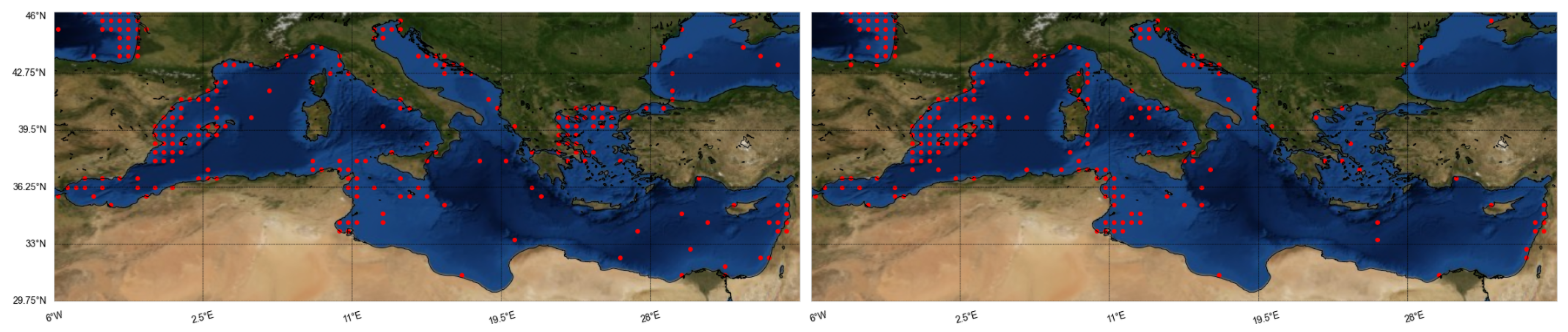
Finally, it is interesting to see what percentage of the Mediterranean Sea is covered by high probability occurrence for each species. Considering 80% and greater as high occurrence probability, following Figure 6, it was computed that anchovy covers 14.7% of the Mediterranean, sardine 17.8%, round sardinella 30.7%, Atlantic chub mackerel 2%, Atlantic mackerel 0.7%, picarel 82.3%, bluefin tuna 4% and swordfish 1.8%. Locations with constant species presence are the Adriatic Sea, the North Aegean Sea, the Alboran Sean, and the sea surrounding the coasts from South France to East Tunisia.

5. Conclusions

Throughout the present study we have presented a comprehensive Species Distribution Model (SDM) for eight commercial pelagic fish species in the Mediterranean Sea. Initial datasets were created by merging several external databases (Aquamaps, CMEMS, EMODnet) in order to produce a model capable of predicting the probability of occurrence in every coordinate pair in the Mediterranean. Ten regression algorithms were compared in order to identify the best performing one, namely XGBoost, which had never previously been used for SDM. With feature engineering, we explored several aspects of the time series data resulting in a large number of features (6830), followed by feature selection with the use of the ensemble Reciprocal Ranking method. After ranking the features, it was found that approximately the top 2% of features were constructing the best model with a 34% performance boosting for the eight species, on average. Feature selection, in combination with the evaluation schema of 10-fold cross validation, reduced the danger of over-fitting and created a robust general model with a cross-validated RMSE ranging from 0.22 to 0.07 depending on the species.

After creating the model, the importance of feature categories and environmental predictors were further explored and discussed. The strongest feature categories are the neighbor-based ones, the features with extreme values (minima, maxima, quantiles), and the monthly and surface features, while the overall strongest predictors are salinity, temperature, distance to coast, dissolved oxygen and nitrate. Finally, using Aquamaps probabilities as target variable, it was improved in both coverage and resolution. High resolution habitat maps were created ($\times 8$ higher) for the whole basin (67,000 points instead of 902) which can be used by researchers to understand the link between marine fishes and environmental factors.

References

1. Hernandez, P.A.; Graham, C.H.; Master, L.L.; Albert, D.L. The effect of sample size and species characteristics on performance of different species distribution modeling methods. Ecography 2006, 29, 773–785. [Google Scholar] [CrossRef]
2. Rassweiler, A.; Costello, C.; Hilborn, R.; Siegel, D.A. Integrating scientific guidance into marine spatial planning. Proc. R. Soc. Biol. Sci. 2014, 281, 20132252. [Google Scholar] [CrossRef] [PubMed]
3. Halpern, B.S.; Lester, S.E.; McLeod, K.L. Placing marine protected areas onto the ecosystem-based management seascape. Proc. Natl. Acad. Sci. USA 2010, 107, 18312–18317. [Google Scholar] [CrossRef] [PubMed] [Green Version]
4. Pearman, P.B.; Guisan, A.; Broennimann, O.; Randin, C.F. Niche dynamics in space and time. Trends Ecol. Evol. 2008, 23, 149–158. [Google Scholar] [CrossRef] [PubMed]
5. Katsanevakis, S.; Zenetos, A.; Belchior, C.; Cardoso, A.C. Invading European Seas: Assessing pathways of introduction of marine aliens. Ocean. Coast. Manag. 2013, 76, 64–74. [Google Scholar] [CrossRef]
6. Cheung, W.W.; Watson, R.; Pauly, D. Signature of ocean warming in global fisheries catch. Nature 2013, 497, 365. [Google Scholar] [CrossRef]
7. Tsikliras, A.C.; Stergiou, K.I. Mean temperature of the catch increases quickly in the Mediterranean Sea. Mar. Ecol. Prog. Ser. 2014, 515, 281–284. [Google Scholar] [CrossRef] [Green Version]
8. FAO. The State of World Fisheries and Aquaculture 2018-Meeting the Sustainable Development Goals; FAO: Rome, Italy, 2018. [Google Scholar]
9. Tsikliras, A.C.; Licandro, P.; Pardalou, A.; McQuinn, I.H.; Gröger, J.P.; Alheit, J. Synchronization of Mediterranean pelagic fish populations with the North Atlantic climate variability. Deep. Sea Res. Part II Top. Stud. Oceanogr. 2019, 159, 143–151. [Google Scholar] [CrossRef]
10. Brosset, P.; Fromentin, J.M.; Van Beveren, E.; Lloret, J.; Marques, V.; Basilone, G.; Bonanno, A.; Carpi, P.; Donato, F.; Keč, V.Č.; et al. Spatio-temporal patterns and environmental controls of small pelagic fish body condition from contrasted Mediterranean areas. Prog. Oceanogr. 2017, 151, 149–162. [Google Scholar] [CrossRef] [Green Version]
11. Alheit, J.; Gröger, J.; Licandro, P.; McQuinn, I.H.; Pohlmann, T.; Tsikliras, A.C. What happened in the mid-1990s? The coupled ocean-atmosphere processes behind climate-induced ecosystem changes in the Northeast Atlantic and the Mediterranean. Deep. Sea Res. Part II Top. Stud. Oceanogr. 2019, 159, 130–142. [Google Scholar] [CrossRef]
12. Hidalgo, M.; Mihneva, V.; Vasconcellos, M.; Bernal, M. Climate change impacts, vulnerabilities and adaptations: Mediterranean Sea and the Black Sea marine fisheries. Impacts Clim. Chang. Fish. Aquac. 2019, 139. [Google Scholar]
13. Saraux, C.; Van Beveren, E.; Brosset, P.; Queiros, Q.; Bourdeix, J.H.; Dutto, G.; Gasset, E.; Jac, C.; Bonhommeau, S.; Fromentin, J.M. Small pelagic fish dynamics: A review of mechanisms in the Gulf of Lions. Deep. Sea Res. Part II Top. Stud. Oceanogr. 2019, 159, 52–61. [Google Scholar] [CrossRef]
14. Lloret, J.; Lleonart, J.; Solé, I.; Fromentin, J.M. Fluctuations of landings and environmental conditions in the north-western Mediterranean Sea. Fish. Oceanogr. 2001, 10, 33–50. [Google Scholar] [CrossRef] [Green Version]
15. Agostini, V.N.; Bakun, A. Ocean triads’ in the Mediterranean Sea: Physical mechanisms potentially structuring reproductive habitat suitability (with example application to European anchovy, Engraulis encrasicolus). Fish. Oceanogr. 2002, 11, 129–142. [Google Scholar] [CrossRef]
16. Bartolino, V.; Colloca, F.; Sartor, P.; Ardizzone, G. Modelling recruitment dynamics of hake, Merluccius merluccius, in the central Mediterranean in relation to key environmental variables. Fish. Res. 2008, 92, 277–288. [Google Scholar] [CrossRef]
17. Coro, G.; Vilas, L.G.; Magliozzi, C.; Ellenbroek, A.; Scarponi, P.; Pagano, P. Forecasting the ongoing invasion of Lagocephalus sceleratus in the Mediterranean Sea. Ecol. Model. 2018, 371, 37–49. [Google Scholar] [CrossRef]
18. Tirelli, T.; Pessani, D. Importance of feature selection in decision-tree and artificial-neural-network ecological applications. Alburnus alburnus alborella: A practical example. Ecol. Inform. 2011, 6, 309–315. [Google Scholar] [CrossRef]
19. Bosch, S.; Tyberghein, L.; Deneudt, K.; Hernandez, F.; De Clerck, O. In search of relevant predictors for marine species distribution modelling using the MarineSPEED benchmark dataset. Divers. Distrib. 2018, 24, 144–157. [Google Scholar] [CrossRef] [Green Version]
20. Leidenberger, S.; Obst, M.; Kulawik, R.; Stelzer, K.; Heyer, K.; Hardisty, A.; Bourlat, S.J. Evaluating the potential of ecological niche modelling as a component in marine non-indigenous species risk assessments. Mar. Pollut. Bull. 2015, 97, 470–487. [Google Scholar] [CrossRef]
21. Moore, C.H.; Harvey, E.S.; Van Niel, K.P. Spatial prediction of demersal fish distributions: Enhancing our understanding of species–environment relationships. ICES J. Mar. Sci. 2009, 66, 2068–2075. [Google Scholar] [CrossRef] [Green Version]
22. Reiss, H.; Cunze, S.; König, K.; Neumann, H.; Kröncke, I. Species distribution modelling of marine benthos: A North Sea case study. Mar. Ecol. Prog. Ser. 2011, 442, 71–86. [Google Scholar] [CrossRef] [Green Version]
23. Wiley, E.O.; McNyset, K.M.; Peterson, A.T.; Robins, C.R.; Stewart, A.M. Niche modeling perspective on geographic range predictions in the marine environment using a machine-learning algorithm. Oceanography 2003, 16, 4. [Google Scholar] [CrossRef] [Green Version]
24. Thorson, J.T.; Ianelli, J.N.; Larsen, E.A.; Ries, L.; Scheuerell, M.D.; Szuwalski, C.; Zipkin, E.F. Joint dynamic species distribution models: A tool for community ordination and spatio-temporal monitoring. Glob. Ecol. Biogeogr. 2016, 25, 1144–1158. [Google Scholar] [CrossRef]
25. Bucklin, D.N.; Basille, M.; Benscoter, A.M.; Brandt, L.A.; Mazzotti, F.J.; Romanach, S.S.; Speroterra, C.; Watling, J.I. Comparing species distribution models constructed with different subsets of environmental predictors. Divers. Distrib. 2015, 21, 23–35. [Google Scholar] [CrossRef]
26. Ferrari, R.; Malcolm, H.A.; Byrne, M.; Friedman, A.; Williams, S.B.; Schultz, A.; Jordan, A.R.; Figueira, W.F. Habitat structural complexity metrics improve predictions of fish abundance and distribution. Ecography 2018, 41, 1077–1091. [Google Scholar] [CrossRef]
27. Effrosynidis, D.; Arampatzis, A.; Sylaios, G. Seagrass and hydrographic data for the Mediterranean Sea. Data Brief 2019, 25, 104286. [Google Scholar] [CrossRef]
28. Coll, M.; Pennino, M.G.; Steenbeek, J.; Solé, J.; Bellido, J.M. Predicting marine species distributions: Complementarity of food-web and Bayesian hierarchical modelling approaches. Ecol. Model. 2019, 405, 86–101. [Google Scholar] [CrossRef]
29. Bradie, J.; Leung, B. A quantitative synthesis of the importance of variables used in MaxEnt species distribution models. J. Biogeogr. 2017, 44, 1344–1361. [Google Scholar] [CrossRef]
30. Báez, J.C.; Olivero, J.; Peteiro, C.; Ferri-Yáñez, F.; Garcia-Soto, C.; Real, R. Macro-environmental modelling of the current distribution of Undaria pinnatifida (Laminariales, Ochrophyta) in northern Iberia. Biol. Invasions 2010, 12, 2131–2139. [Google Scholar] [CrossRef]
31. Elith, J.; Graham, C.H.; Anderson, R.P.; Dudík, M.; Ferrier, S.; Guisan, A.; Hijmans, R.J.; Huettmann, F.; Leathwick, J.; Lehmann, A.; et al. Novel methods improve prediction of species’ distributions from occurrence data. Ecography 2006, 29, 129–151. [Google Scholar] [CrossRef] [Green Version]
32. Chen, T.; Guestrin, C. Xgboost: A scalable tree boosting system. In Proceedings of the 22nd ACM Sigkdd International Conference on Knowledge Discovery and Data Mining, San Francisco, CA, USA, 13–17 August 2016; ACM: New York, NY, USA, 2016; pp. 785–794. [Google Scholar]
33. Von Schuckmann, K.; Le Traon, P.Y.; Alvarez-Fanjul, E.; Axell, L.; Balmaseda, M.; Breivik, L.A.; Brewin, R.J.; Bricaud, C.; Drevillon, M.; Drillet, Y.; et al. The Copernicus marine environment monitoring service ocean state report. J. Oper. Oceanogr. 2016, 9, s235–s320. [Google Scholar] [CrossRef]
34. EMODnet Bathymetry Consortium. EMODnet Digital Bathymetry (DTM). Emodnet Bathymetry 2016, 10. [Google Scholar]
35. Emig, C.; Geistdoerfer, P. The Mediterranean deep-sea fauna: Historical evolution, bathymetric variations and geographical changes. arXiv 2005, arXiv:q-bio/0507003. [Google Scholar] [CrossRef]
36. Bosc, E.; Bricaud, A.; Antoine, D. Seasonal and interannual variability in algal biomass and primary production in the Mediterranean Sea, as derived from 4 years of SeaWiFS observations. Glob. Biogeochem. Cycles 2004, 18. [Google Scholar] [CrossRef] [Green Version]
37. Tintoré, J.; Pinardi, N.; Alvarez Fanjul, E.; Balbin, R.; Bozzano, R.; Ferrarin, C.; Bajo, M.; Cardin, V.R.; Charcos Llorens, M.V.; Chiggiato, J.; et al. Challenges for Sustained Observing and Forecasting Systems in the Mediterranean Sea. Front. Mar. Sci. 2019, 6, 568. [Google Scholar] [CrossRef] [Green Version]
38. Coll, M.; Piroddi, C.; Steenbeek, J.; Kaschner, K.; Lasram, F.B.R.; Aguzzi, J.; Ballesteros, E.; Bianchi, C.N.; Corbera, J.; Dailianis, T.; et al. The biodiversity of the Mediterranean Sea: Estimates, patterns, and threats. PLoS ONE 2010, 5, e11842. [Google Scholar] [CrossRef] [Green Version]
39. Kaschner, K.; Ready, J.; Agbayani, E.; Rius, J.; Kesner-Reyes, K.; Eastwood, P.; South, A.; Kullander, S.; Rees, T.; Close, C.; et al. AquaMaps: Predicted range maps for aquatic species. World Wide Web Electron. Publ. Wwwaquamapsorg. Version 2008, 10, 2008. [Google Scholar]
40. Politikos, D.V.; Triantafyllou, G.; Petihakis, G.; Tsiaras, K.; Somarakis, S.; Ito, S.I.; Megrey, B.A. Application of a bioenergetics growth model for European anchovy (Engraulis encrasicolus) linked with a lower trophic level ecosystem model. Hydrobiologia 2011, 670, 141–163. [Google Scholar] [CrossRef]
41. Tsikliras, A.C.; Koutrakis, E.T. Growth and reproduction of European sardine, Sardina pilchardus (Pisces: Clupeidae), in northeastern Mediterranean. Cah. Biol. Mar. 2013, 54, 365–374. [Google Scholar]
42. Alheit, J.; Licandro, P.; Coombs, S.; Garcia, A.; Giráldez, A.; Santamaría, M.T.G.; Slotte, A.; Tsikliras, A.C. Reprint of “Atlantic Multidecadal Oscillation (AMO) modulates dynamics of small pelagic fishes and ecosystem regime shifts in the eastern North and Central Atlantic”. J. Mar. Syst. 2014, 133, 88–102. [Google Scholar] [CrossRef] [Green Version]
43. Tsikliras, A.C.; Antonopoulou, E. Reproductive biology of round sardinella (Sardinella aurita) in north-eastern Mediterranean. Sci. Mar. 2006, 70, 281–290. [Google Scholar] [CrossRef] [Green Version]
44. Tsikliras, A.C.; Torre, M.; Stergiou, K.I. Feeding habits and trophic level of round sardinella (Sardinella aurita) in the northeastern Mediterranean (Aegean Sea, Greece). J. Biol. Res. 2005, 3, 67–75. [Google Scholar]
45. Sabatés, A.; Martín, P.; Lloret, J.; Raya, V. Sea warming and fish distribution: The case of the small pelagic fish, Sardinella aurita, in the western Mediterranean. Glob. Chang. Biol. 2006, 12, 2209–2219. [Google Scholar] [CrossRef]
46. Tsikliras, A.C. Chasing after the high impact. Ethics Sci. Environ. Politics 2008, 8, 45–47. [Google Scholar] [CrossRef] [Green Version]
47. Tsikliras, A.C.; Antonopoulou, E.; Stergiou, K.I. Spawning period of Mediterranean marine fishes. Rev. Fish Biol. Fish. 2010, 20, 499–538. [Google Scholar] [CrossRef]
48. Froese, R. FishBase. World Wide Web Electronic Publication. Available online: http://www.fishbase.org (accessed on 20 March 2020).
49. Juntunen, T.; Tsikliras, A.; Mantyniemi, S.; Stergiou, K. A Bayesian population model to estimate changes in the stock size in data poor cases using Mediterranean bogue (Boops boops) and picarel (Spicara smaris) as an example. Mediterr. Mar. Sci. 2014, 15, 587–601. [Google Scholar] [CrossRef] [Green Version]
50. Karakulak, S.; Oray, I.; Corriero, A.; Deflorio, M.; Santamaria, N.; Desantis, S.; De Metrio, G. Evidence of a spawning area for the bluefin tuna (Thunnus thynnus L.) in the eastern Mediterranean. J. Appl. Ichthyol. 2004, 20, 318–320. [Google Scholar] [CrossRef]
51. Corriero, A.; Karakulak, S.; Santamaria, N.; Deflorio, M.; Spedicato, D.; Addis, P.; Desantis, S.; Cirillo, F.; Fenech-Farrugia, A.; Vassallo-Agius, R.; et al. Size and age at sexual maturity of female bluefin tuna (Thunnus thynnus L. 1758) from the Mediterranean Sea. J. Appl. Ichthyol. 2005, 21, 483–486. [Google Scholar] [CrossRef]
52. MacKenzie, B.R.; Mosegaard, H.; Rosenberg, A.A. Impending collapse of bluefin tuna in the northeast Atlantic and Mediterranean. Conserv. Lett. 2009, 2, 26–35. [Google Scholar] [CrossRef]
53. Tserpes, G.; Peristeraki, P.; Valavanis, V.D. Distribution of swordfish in the eastern Mediterranean, in relation to environmental factors and the species biology. Hydrobiologia 2008, 612, 241. [Google Scholar] [CrossRef]
54. Alıçlı, T.Z.; Oray, I.K.; Karakulak, F.S.; Kahraman, A.E. Age, sex ratio, length-weight relationships and reproductive biology of Mediterranean swordfish, Xiphias gladius L., 1758, in the eastern Mediterranean. Afr. J. Biotechnol. 2012, 11, 3673–3680. [Google Scholar]
55. Corsi, F.; De Leeuw, J.; Skidmore, A. Modeling Species Distribution with GIS. In Research Techniques in Animal Ecology: Controversies and Consequences; Boitani, L., Fuller, T.K., Eds.; Columbia University Press: New York, NY, USA, 2000. [Google Scholar]
56. Ready, J.; Kaschner, K.; South, A.B.; Eastwood, P.D.; Rees, T.; Rius, J.; Agbayani, E.; Kullander, S.; Froese, R. Predicting the distributions of marine organisms at the global scale. Ecol. Model. 2010, 221, 467–478. [Google Scholar] [CrossRef]
57. Austin, M. Species distribution models and ecological theory: A critical assessment and some possible new approaches. Ecol. Model. 2007, 200, 1–19. [Google Scholar] [CrossRef]
58. Planque, B.; Buffaz, L. Quantile regression models for fish recruitment–environment relationships: Four case studies. Mar. Ecol. Prog. Ser. 2008, 357, 213–223. [Google Scholar] [CrossRef] [Green Version]
59. Effrosynidis, D.; Arampatzis, A.; Sylaios, G. Seagrass detection in the mediterranean: A supervised learning approach. Ecol. Inform. 2018, 48, 158–170. [Google Scholar] [CrossRef]
60. Assis, J.; Tyberghein, L.; Bosch, S.; Verbruggen, H.; Serrão, E.A.; De Clerck, O. Bio-ORACLE v2. 0: Extending marine data layers for bioclimatic modelling. Glob. Ecol. Biogeogr. 2018, 27, 277–284. [Google Scholar] [CrossRef]
61. Reygondeau, G.; Guieu, C.; Benedetti, F.; Irisson, J.O.; Ayata, S.D.; Gasparini, S.; Koubbi, P. Biogeochemical regions of the Mediterranean Sea: An objective multidimensional and multivariate environmental approach. Prog. Oceanogr. 2017, 151, 138–148. [Google Scholar] [CrossRef] [Green Version]
62. Froese, R.; Winker, H.; Coro, G.; Demirel, N.; Tsikliras, A.C.; Dimarchopoulou, D.; Scarcella, G.; Quaas, M.; Matz-Lück, N. Status and rebuilding of European fisheries. Mar. Policy 2018, 93, 159–170. [Google Scholar] [CrossRef]
63. Cury, P.; Bakun, A.; Crawford, R.J.; Jarre, A.; Quinones, R.A.; Shannon, L.J.; Verheye, H.M. Small pelagics in upwelling systems: Patterns of interaction and structural changes in “wasp-waist” ecosystems. ICES J. Mar. Sci. 2000, 57, 603–618. [Google Scholar] [CrossRef]
64. Albo-Puigserver, M.; Navarro, J.; Coll, M.; Layman, C.A.; Palomera, I. Trophic structure of pelagic species in the northwestern Mediterranean Sea. J. Sea Res. 2016, 117, 27–35. [Google Scholar] [CrossRef]
65. Palomera, I.; Olivar, M.P.; Salat, J.; Sabatés, A.; Coll, M.; García, A.; Morales-Nin, B. Small pelagic fish in the NW Mediterranean Sea: An ecological review. Prog. Oceanogr. 2007, 74, 377–396. [Google Scholar] [CrossRef]
66. Kokkos, N.; Sylaios, G. Modeling the buoyancy-driven Black Sea water outflow into the North Aegean Sea. Oceanologia 2016, 58, 103–116. [Google Scholar] [CrossRef] [Green Version]
67. Danovaro, R.; Dinet, A.; Duineveld, G.; Tselepides, A. Benthic response to particulate fluxes in different trophic environments: A comparison between the Gulf of Lions–Catalan Sea (western-Mediterranean) and the Cretan Sea (eastern-Mediterranean). Prog. Oceanogr. 1999, 44, 287–312. [Google Scholar] [CrossRef]
68. Coll, M.; Piroddi, C.; Albouy, C.; Ben Rais Lasram, F.; Cheung, W.W.; Christensen, V.; Karpouzi, V.S.; Guilhaumon, F.; Mouillot, D.; Paleczny, M.; et al. The Mediterranean Sea under siege: Spatial overlap between marine biodiversity, cumulative threats and marine reserves. Glob. Ecol. Biogeogr. 2012, 21, 465–480. [Google Scholar] [CrossRef]
69. Molinero, J.C.; Ibanez, F.; Nival, P.; Buecher, E.; Souissi, S. North Atlantic climate and northwestern Mediterranean plankton variability. Limnol. Oceanogr. 2005, 50, 1213–1220. [Google Scholar] [CrossRef]
70. Van Beveren, E.; Bonhommeau, S.; Fromentin, J.M.; Bigot, J.L.; Bourdeix, J.H.; Brosset, P.; Roos, D.; Saraux, C. Rapid changes in growth, condition, size and age of small pelagic fish in the Mediterranean. Mar. Biol. 2014, 161, 1809–1822. [Google Scholar] [CrossRef] [Green Version]
71. Brosset, P.; Ménard, F.; Fromentin, J.M.; Bonhommeau, S.; Ulses, C.; Bourdeix, J.H.; Bigot, J.L.; Van Beveren, E.; Roos, D.; Saraux, C. Influence of environmental variability and age on the body condition of small pelagic fish in the Gulf of Lions. Mar. Ecol. Prog. Ser. 2015, 529, 219–231. [Google Scholar] [CrossRef] [Green Version]
72. Jghab, A.; Vargas-Yañez, M.; Reul, A.; Garcia-Martínez, M.; Hidalgo, M.; Moya, F.; Bernal, M.; Omar, M.B.; Benchoucha, S.; Lamtai, A. The influence of environmental factors and hydrodynamics on sardine (Sardina pilchardus, Walbaum 1792) abundance in the southern Alboran Sea. J. Mar. Syst. 2019, 191, 51–63. [Google Scholar] [CrossRef]
73. Giannoulaki, M.; Pyrounaki, M.M.; Liorzou, B.; Leonori, I.; Valavanis, V.D.; Tsagarakis, K.; Bigot, J.L.; Roos, D.; De Felice, A.; Campanella, F.; et al. Habitat suitability modelling for sardine juveniles (Sardina pilchardus) in the Mediterranean Sea. Fish. Oceanogr. 2011, 20, 367–382. [Google Scholar] [CrossRef] [Green Version]
74. Erauskin-Extramiana, M.; Arrizabalaga, H.; Cabré, A.; Coelho, R.; Rosa, D.; Ibaibarriaga, L.; Chust, G. Are shifts in species distribution triggered by climate change? A swordfish case study. Deep. Sea Res. Part II Top. Stud. Oceanogr. 2019, 175, 104666. [Google Scholar] [CrossRef]
75. Lauriano, G.; Pierantonio, N.; Kell, L.; Cañadas, A.; Donovan, G.; Panigada, S. Fishery-independent surface abundance and density estimates of swordfish (Xiphias gladius) from aerial surveys in the Central Mediterranean Sea. Deep. Sea Res. Part II Top. Stud. Oceanogr. 2017, 141, 102–114. [Google Scholar] [CrossRef]
76. Faillettaz, R.; Beaugrand, G.; Goberville, E.; Kirby, R.R. Atlantic Multidecadal Oscillations drive the basin-scale distribution of Atlantic bluefin tuna. Sci. Adv. 2019, 5, eaar6993. [Google Scholar] [CrossRef] [PubMed] [Green Version]
77. Allain, G.; Petitgas, P.; Lazure, P. The influence of environment and spawning distribution on the survival of anchovy (Engraulis encrasicolus) larvae in the Bay of Biscay (NE Atlantic) investigated by biophysical simulations. Fish. Oceanogr. 2007, 16, 506–514. [Google Scholar] [CrossRef] [Green Version]
78. Tugores, M.P.; Giannoulaki, M.; Iglesias, M.; Bonanno, A.; Tičina, V.; Leonori, I.; Machias, A.; Tsagarakis, K.; Diaz, N.; Giraldez, A.; et al. Habitat suitability modelling for sardine Sardina pilchardus in a highly diverse ecosystem: The Mediterranean Sea. Mar. Ecol. Prog. Ser. 2011, 443, 181–205. [Google Scholar] [CrossRef] [Green Version]
79. Giannoulaki, M.; Iglesias, M.; Tugores, M.P.; Bonanno, A.; Patti, B.; De Felice, A.; Leonori, I.; Bigot, J.L.; Tičina, V.; Pyrounaki, M.; et al. Characterizing the potential habitat of European anchovy Engraulis encrasicolus in the Mediterranean Sea, at different life stages. Fish. Oceanogr. 2013, 22, 69–89. [Google Scholar] [CrossRef]
80. Martín, P.; Sabatés, A.; Lloret, J.; Martin-Vide, J. Climate modulation of fish populations: The role of the Western Mediterranean Oscillation (WeMO) in sardine (Sardina pilchardus) and anchovy (Engraulis encrasicolus) production in the north-western Mediterranean. Clim. Chang. 2012, 110, 925–939. [Google Scholar] [CrossRef]
81. Schwartzlose, R.; Alheit, J. Worldwide large-scale fluctuations of sardine and anchovy populations. Afr. J. Mar. Sci. 1999, 21, 195–205. [Google Scholar] [CrossRef]
82. Katara, I.; Pierce, G.J.; Illian, J.; Scott, B.E. Environmental drivers of the anchovy/sardine complex in the Eastern Mediterranean. Hydrobiologia 2011, 670, 49–65. [Google Scholar] [CrossRef]
83. Calvo, E.; Simó, R.; Coma, R.; Ribes, M.; Pascual, J.; Sabatés, A.; Gili, J.M.; Pelejero, C. Effects of climate change on Mediterranean marine ecosystems: The case of the Catalan Sea. Clim. Res. 2011, 50, 1–29. [Google Scholar] [CrossRef] [Green Version]
84. Martín, P.; Bahamon, N.; Sabatés, A.; Maynou, F.; Sánchez, P.; Demestre, M. European anchovy (Engraulis encrasicolus) landings and environmental conditions on the Catalan Coast (NW Mediterranean) during 2000–2005. In Essential Fish Habitat Mapping in the Mediterranean; Springer: Berlin/Heidelberg, Germany, 2008; pp. 185–199. [Google Scholar]
85. Martin-Vide, J.; Lopez-Bustins, J.A. The western Mediterranean oscillation and rainfall in the Iberian Peninsula. Int. J. Climatol. J. R. Meteorol. Soc. 2006, 26, 1455–1475. [Google Scholar] [CrossRef]
86. Tsikliras, A.C. Sympatric Clupeoid Fish Larvae in the Northeastern Mediterranean: Coexistence or Avoidance? Adv. Ecol. 2014, 2014. [Google Scholar] [CrossRef]
87. Palomera, I. Co-oeeurrenee of Engraulis encrasicolus and Sardinella aurita eggs and larvae in the northwestern Mediterranean. Citac. Sci. Mar. 1990, 54, 61–67. [Google Scholar]
88. Morote, E.; Olivar, M.P.; Villate, F.; Uriarte, I. Diet of round sardinella, Sardinella aurita, larvae in relation to plankton availability in the NW Mediterranean. J. Plankton Res. 2008, 30, 807–816. [Google Scholar] [CrossRef]
89. Cury, P.; Fontana, A. Compétition et stratégies démographiques comparées de deux espèces de sardinelles (Sardinella aurita et Sardinella maderensis) des côtes ouest-africaines. Aquat. Living Resour. 1988, 1, 165–180. [Google Scholar] [CrossRef]
90. Sabates, A.; Olivar, M.P.; Salat, J.; Palomera, I.; Alemany, F. Physical and biological processes controlling the distribution of fish larvae in the NW Mediterranean. Prog. Oceanogr. 2007, 74, 355–376. [Google Scholar] [CrossRef] [Green Version]
Figure 1. Occurrence points used by Aquamaps to create the environmental envelope for Engraulis encrasicolus (left) and Sardina pilchardus (right). The points inside the Mediterranean are used by the machine learning models in this study for training and evaluation. The dependent variable is the probability of occurrence extracted from AquaMaps for each point and the independent variables are the environmental conditions regarding these locations extracted from other platforms.
Applsci 10 08900 g001
Figure 2. Graphical representation of the proposed procedure. First, data are collected from AquaMaps, which make the target variable. For these points, environmental parameters that serve as dependent variables are extracted from platforms such as CMES and EMODnet. Data are spatially filtered in the Mediterranean Sea. Next, feature engineering is performed, and after that, feature selection to reduce the number of variables to the optimum. Finally, using the model that was trained, predictions for the probability of the species are performed in every point of the Mediterranean at a fine resolution. Example values are for Engraulis encrasicolus.
Applsci 10 08900 g002
Figure 3. Root Mean Square Error (RMSE) of the predictions for the eight species as the number of features (%) decreases. This is a backward stepwise selection process, starting from all features up to 0.01% of them, with a step of 0.01% reduction. The importance of the features is the outcome of the Reciprocal Ranking. The optimal number of features for all species is arounf 2%.
Applsci 10 08900 g003
Figure 4. Importance (as indicated by Reciprocal Ranking) of feature categories generated by the feature engineering procedure. The lower the value, the better. It is evident that some categories are superior than others, and some are to be avoided.
Applsci 10 08900 g004
Figure 5. Strengths (the further from the center, the stronger) of the top-10 most important predictors for each species. From top-left to bottom-right the species are: Engraulis encrasicolus, Sardina pilchardus, Sardinella aurita, Scomber colias, Scomber scombrus, Spicara smaris, Thunnus thynnus, Xiphias gladius.
Applsci 10 08900 g005
Figure 6. High resolution produced habitat maps depicting the probability of occurrence in the whole Mediterranean Sea for the eight commercial fish species. Each unknown point was predicted using the final trained model of the proposed work.
Applsci 10 08900 g006