Article

Cable Tension Analysis Oriented the Enhanced Stiffness of a 3-DOF Joint Module of a Modular Cable-Driven Human-Like Robotic Arm

1
School of Mechanical Engineering and Mechanics, Ningbo University, Ningbo 315211, China
2
Zhejiang Key Lab of Robotics and Intelligent Manufacturing Equipment Technology, Ningbo Institute of Material Technology and Engineering, Chinese Academy of Sciences (CAS), Ningbo 315201, China
3
Zhejiang Marine Development Research Institute, Zhoushan 316021, China
4
Ningbo Artificial Intelligence Institute, Shanghai Jiao Tong University, Ningbo 315000, China
*
Authors to whom correspondence should be addressed.
Appl. Sci. 2020, 10(24), 8871; https://doi.org/10.3390/app10248871
Submission received: 18 November 2020 / Revised: 5 December 2020 / Accepted: 7 December 2020 / Published: 11 December 2020
(This article belongs to the Special Issue Advances in Bio-Inspired Robots)

Abstract

:
Inspired by the structure of human arms, a modular cable-driven human-like robotic arm (CHRA) is developed for safe human–robot interaction. Due to the unilateral driving properties of the cables, the CHRA is redundantly actuated and its stiffness can be adjusted by regulating the cable tensions. Since the trajectory of the 3-DOF joint module (3DJM) of the CHRA is a curve on Lie group SO(3), an enhanced stiffness model of the 3DJM is established by the covariant derivative of the load to the displacement on SO(3). In this paper, we focus on analyzing the how cable tension distribution problem oriented the enhanced stiffness of the 3DJM of the CHRA for stiffness adjustment. Due to the complexity of the enhanced stiffness model, it is difficult to solve the cable tensions from the desired stiffness analytically. The problem of stiffness-oriented cable tension distribution (SCTD) is formulated as a nonlinear optimization model. The optimization model is simplified using the symmetry of the enhanced stiffness model, the rank of the Jacobian matrix and the equilibrium equation of the 3DJM. Since the objective function is too complicated to compute the gradient, a method based on the genetic algorithm is proposed for solving this optimization problem, which only utilizes the objective function values. A comprehensive simulation is carried out to validate the effectiveness of the proposed method.

1. Introduction

Unlike conventional robots that work in structured environments, safe human–robot interactions have been a key element for the robots that work in unstructured and unpredictable environments. Inspired by the structure of human arms, a modular 
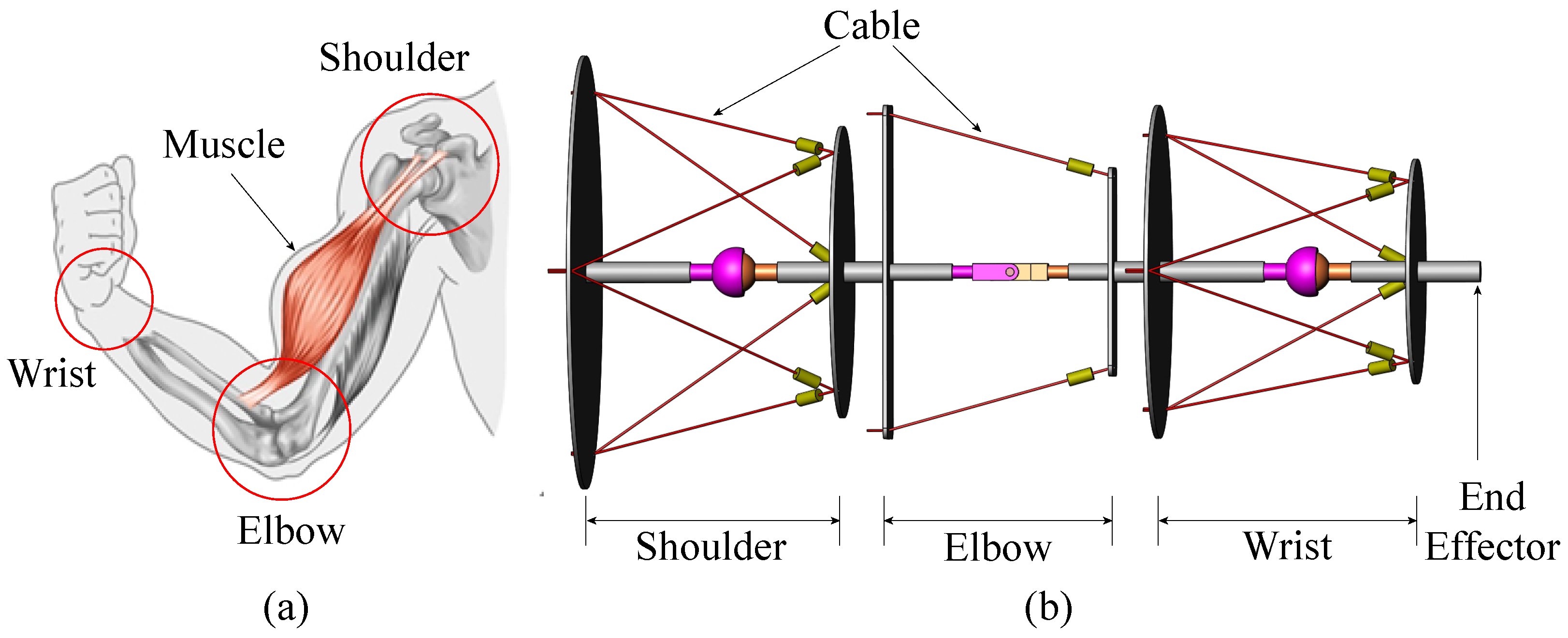
cable-driven human-like robotic arm (CHRA) is developed for safe human–robot interaction, which employs cables to mimic the functionality of the human muscles. As shown in Figure 1, the CHRA consists of a shoulder joint, an elbow joint and a wrist joint in series, where the shoulder joint and the wrist joint have three degrees of freedom (3-DOF) and the elbow joint has one degree of freedom (1-DOF). The CHRA employs lightweight cables to drive the rigid links and the cables can be wound into winches mounted onto the base of the CHRA. A variable-stiffness device (VSD) is designed and placed along with each driving cable to increase the flexibility of the cables. With these arrangements, the CHRA has flexibility advantages [1], low moving mass [2], large workspace [3] and high payload-to-weight ratio [4]. Due to these advantages, the CHRA is intrinsically safe for human–robot interactions. The proposed CHRA and its joint modules are one kind of cable-driven mechanisms (CDMs). In the last decades, various CDMs have been designed for various applications, such as medical robots [5,6,7], rehabilitation robots [8,9,10,11,12], inspection and repair [13,14,15], and moving payloads [16,17,18,19].
Unlike rigid links, the cables have the unilateral driving property (i.e., they can only pull, but can not push). Hence, the CHRA and its joint modules are redundantly actuated. For a given pose, a lot of cable tension solutions are feasible for the CHRA. Furthermore, the stiffness of the CHRA can be adjusted by regulating the cable tensions. The characteristic of variable stiffness increases the flexibility and safety of the CHRA.
The problem of stiffness-oriented cable tension distribution (SCTD) of a CDM aims at finding the optimal cable tensions to achieve a desired stiffness. However, in the last decades, most studies on cable tension distribution have been carried out to minimize the cable tensions to reduce the energy consumption [20,21,22,23,24,25,26,27]. In [28], the SCTD problem of a CDM was studied by formulating it as an optimization model, and a gradient-projection-based algorithm was presented to solve the optimization problem. However, it utilized the determinant of the stiffness matrix as the objective function. With this method, the desired stiffness cannot be achieved accurately. In [29], the SCTD problem of a 3-DOF cable-driven spherical mechanism was studied and it established the optimization model with all entries of the stiffness matrix, not only the determinant of the stiffness matrix. However, it employed the conventional stiffness model of the CDM, which was derived by the conventional differential formula of the load to the displacement. Since the trajectory of the 3-DOF cable-driven spherical mechanism is a curve on Lie group SO(3) and SO(3) is nonlinear, the stiffness model based on the conventional differential formula is not exactly accurate on SO(3). Its stiffness should be evaluated by the variation of its load against its displacement on SO(3).
In order to study the SCTD problem of the proposed CHRA, the SCTD problems of the 1-DOF and 3-DOF joint modules should be studied first. Due to the simple structure of the 1-DOF joint module, its SCTD problem can be solved easily. For the 3-DOF joint module (3DJM) of the CHRA, its trajectory is a curve on SO(3). We derive the stiffness model of the 3DJM by the covariant derivative of the load to the displacement on SO(3), and call it the enhanced stiffness model of the 3DJM. In this paper, we focus on investigating how the cable tension distribution problem oriented the enhanced stiffness of the 3DJM. Due the complexity of the enhanced stiffness model, it is difficult to solve the cable tensions from the desired stiffness of the 3DJM analytically. We formulate the SCTD problem of the 3DJM as a nonlinear constrained optimization problem. Due to the symmetry of the enhanced stiffness model of the 3DJM, the desired stiffness matrix can be transformed to a diagonal matrix by an orthogonal transformation. Based on the analysis of the rank of the Jacobian matrix of the 3DJM, the six cables can be divided into two groups: one group with three cables for position adjustment by regulating the cable lengths, and another group with the remaining three cables for stiffness adjustment by regulating the cable tensions. In this manner, the position and stiffness of the 3DJM can be adjusted simultaneously. Furthermore, three cable tensions for position adjustment can be expressed by another three cable tensions for stiffness adjustment using the equilibrium equation of the 3DJM. That means the six decision variables of the optimization model can be reduced to three. Since the objective function of the optimization model is too complicated to compute the gradient, a direct optimization method based on the genetic algorithm is proposed for solving the optimization problem, which only utilizes the objective function values. A comprehensive simulation is carried out to validate the effectiveness of the proposed method. The results show that the proposed method provides an accurate and efficient way to adjust the stiffness of the 3DJM by regulating the cable tensions. In summary, the main contribution of this paper is solving the cable tension distribution problem with the enhanced stiffness model of the 3DJM using a method based on the genetic algorithm.

2. Enhanced Stiffness Model of the 3DJM

As shown in 
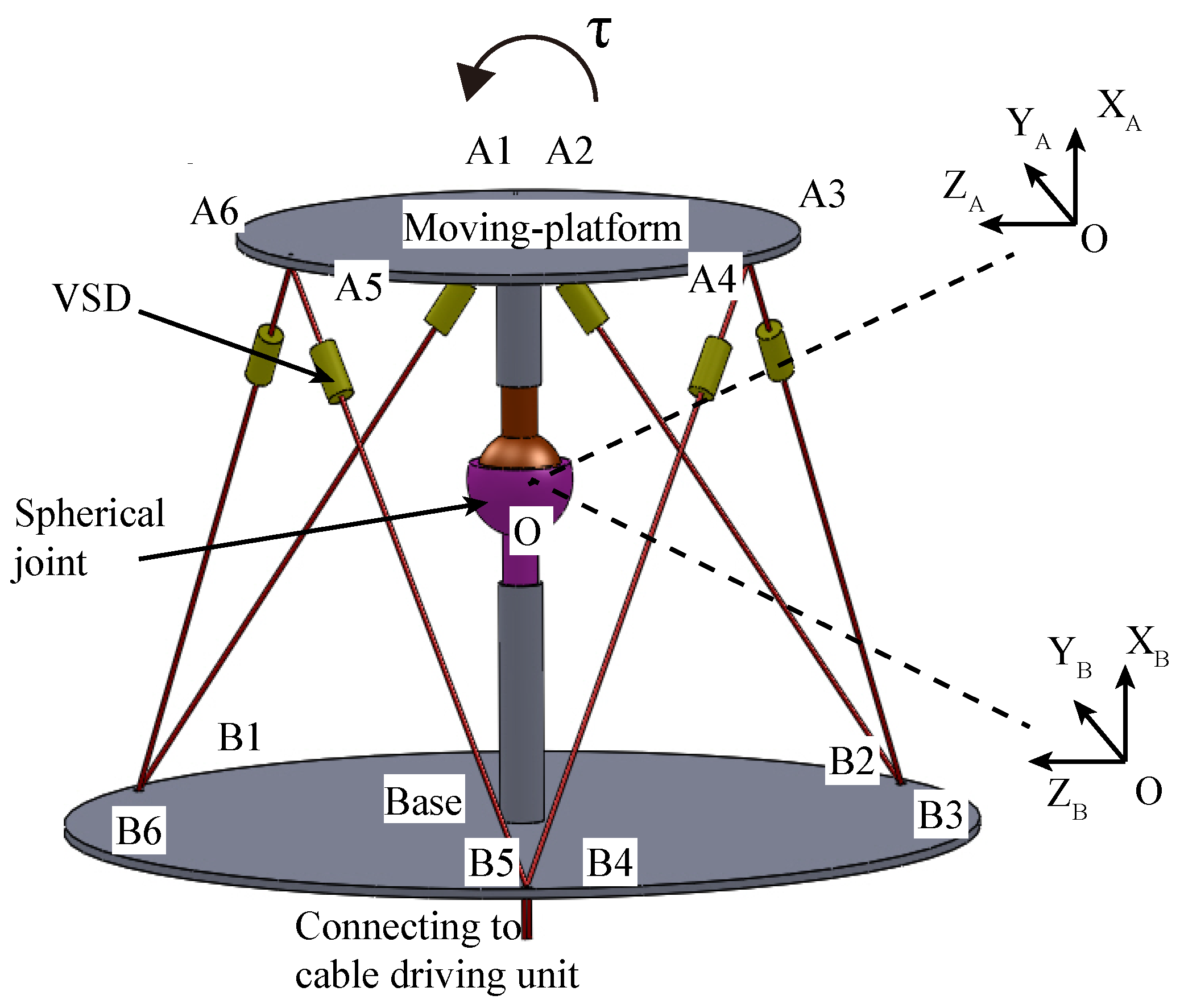
Figure 2, the 3-DOF joint module (3DJM) of the CHRA was made up with a base, a moving-platform and a passive spherical joint connecting them. Six cables were employed to drive the moving-platform and a variable-stiffness device (VSD) was placed along with each driving cable. For routing the cables, six small holes were drilled in the moving-platform and the base, denoted by A i and B i ( i = 1 , 2 , , 6 ) , respectively. In this design, A 2 A 3 = A 4 A 5 = A 6 A 1 = l A , B 1 B 2 = B 3 B 4 = B 5 B 6 = l B , A 1 A 2 = A 3 A 4 = A 5 A 6 = e A , B 2 B 3 = B 4 B 5 = B 6 B 1 = e B , where e A 0 and e B 0 . The distance between the moving-platform and the spherical joint is denoted as h A R , and the distance between the base and the spherical joint is denoted as h B R . Each cable was actuated by a cable driving unit.
To describe the pose of the 3DJM, two frames were attached to the moving-platform (named moving frame {A}) and the base (named base frame {B}), which were both located at the center of the joint O. With the two frames, the pose of the 3DJM can be represented by a rotation matrix R S O ( 3 ) . Thus, the motion trajectory of the 3DJM was a parameterized curve R ( t ) on S O ( 3 ) . The enhanced stiffness model of the 3DJM was established by using the covariant derivative of the load to the displacement on SO(3) [30].

2.1. Displacement and Load of the 3DJM on SO(3)

According to the exponential formula [31], the trajectory curve of the 3DJM R ( t ) yields
R ( t ) = e ζ ^ ( t ) ,
where ζ ^ s o ( 3 ) is an element of Lie algebra s o ( 3 ) and satisfies
ζ = ζ 1 ζ 2 ζ 3 ζ ^ = 0 ζ 3 ζ 2 ζ 3 0 ζ 1 ζ 2 ζ 1 0 .
Here, ζ R 3 is called the coordinates of ζ ^ s o ( 3 ) . The derivative of R ( t ) to time t, i.e., R ˙ ( t ) , is an element of the tangent space of S O ( 3 ) at the point R ( t ) , denoted as T R ( t ) S O ( 3 ) . According to (1), R ˙ ( t ) satisfies the following equation
R ˙ ( t ) = R ( t ) ζ ˙ ^ ( t ) = R ( t ) ω ^ ( t ) ,
where ω ( t ) = ζ ˙ ( t ) s o ( 3 ) is the angular velocity of the 3DJM. Given e ^ j ( j = 1 , 2 , 3 ) as the basis of s o ( 3 ) , where e 1 = ( 1 , 0 , 0 ) T , e 2 = ( 0 , 1 , 0 ) T and e 3 = ( 0 , 0 , 1 ) T , then R ˙ ( t ) can be expressed as
R ˙ ( t ) = R ( t ) ω ^ ( t ) = R ( t ) j = 1 3 ω j e ^ j = j = 1 3 ω j R ( t ) e ^ j = j = 1 3 ω j L j | R ( t ) ,
where L j | R ( t ) = R ( t ) e ^ j ( j = 1 , 2 , 3 ) are taken as the basis of T R ( t ) S O ( 3 ) and L j | R ( t ) are always written as L j for short. From (4), it can be concluded that T R ( t ) S O ( 3 ) is isomorphic to s o ( 3 ) .
Since R ˙ ( t ) describes the velocity of the 3DJM, the instantaneous displacement of the 3DJM can be represented by δ R , yielding
δ R ( t ) = R ˙ ( t ) δ t .
That means the instantaneous displacement of the 3DJM can be described on the tangent space of S O ( 3 ) . Similarly, since the moment load τ ^ is an element of s o * ( 3 ) , the dual space of s o ( 3 ) , by analogy with ω ^ s o ( 3 ) and R ˙ ( t ) T R ( t ) S O ( 3 ) , we define F ( t ) = R ( t ) τ ^ ( t ) as an element of the dual space of the tangent space T R ( t ) S O ( 3 ) at R ( t ) , called cotangent space and denoted as T R ( t ) * S O ( 3 ) . The element of the cotangent space is named as the cotangent vector. Given λ ^ k ( k = 1 , 2 , 3 ) as the basis of s o * ( 3 ) and Λ k | R ( t ) = R ( t ) λ ^ k ( k = 1 , 2 , 3 ) as the basis of T R ( t ) * S O ( 3 ) , then F ( t ) T R ( t ) * S O ( 3 ) satisfies
F ( t ) = R ( t ) τ ^ ( t ) = k = 1 3 τ k R ( t ) λ ^ k = k = 1 3 τ k Λ k | R ( t ) .
It shows that T R ( t ) * S O ( 3 ) is isomorphic to s o * ( 3 ) . Thus, F ( t ) can be employed to represent the load applied on the 3DJM. That means the load applied on the 3DJM can be described on the cotangent space of S O ( 3 ) .

2.2. Enhanced Stiffness Model of the 3DJM on SO(3)

According to the definition, the stiffness of the 3DJM is evaluated by the variation of its load against its displacement. However, the loads and displacements for different poses of the 3DJM are in different cotangent spaces and tangent spaces of SO(3). Considering the property of the motion of the 3DJM, an affine connection called Levi-Civita connection is introduced into S O ( 3 ) to connect different tangent spaces on SO(3) [32]. Given a curve R ( t ) and a vector field V ( t ) on S O ( 3 ) , the affine connection specifies how a vector V ( t 0 ) in the tangent space at point R ( t 0 ) can be mapped to another vector V t 0 ( t 1 ) of the tangent space at some other point R ( t 1 ) . The vector V t 0 ( t 1 ) is called the parallel transport of V ( t 0 ) along the curve R ( t ) [33]. Then, a differentiation operation can be defined on SO(3) as below
R ˙ V | R ( t 0 ) = lim t 1 t 0 V t 0 ( t 1 ) V ( t 0 ) t 1 t 0 ,
where R ˙ V | R ( t 0 ) is called the covariant derivative of V ( t ) along the curve R ( t ) . For two vectors, V 1 and V 2 , in the tangent spaces of SO(3), V 2 V 1 is employed to represent the covariant derivative of V 1 in the direction V 2 . For a real-valued function f on S O ( 3 ) , the covariant derivative V f is usually written as V f . According to the property of covariant derivative, the covariant derivative of the load F ( t ) to the instantaneous displacement δ R ( t ) can be written as
δ R ( t ) F = R ˙ ( t ) δ t F = δ t j = 1 3 ω j L j F = δ t j = 1 3 ω j L j F = δ t K ω = K δ ζ ,
and K = ( L 1 F , L 2 F , L 3 F ) R 3 × 3 is employed as the stiffness of the 3DJM. The components of the stiffness matrix K , i.e., K j k ( j , k = 1 , 2 , 3 ) , yield
K j k = L k F , L j .
According to the property of the Levi–Civita connection [30], we have
K j k = L k F , L j F , L k L j = L k τ j 1 2 r = 1 3 τ r γ k j r ,
where the coefficients γ k j r ( j , k , r = 1 , 2 , 3 ) R are zero except
γ 12 3 = γ 31 2 = γ 23 1 = 2 , γ 21 3 = γ 13 2 = γ 32 1 = 2 .
Furthermore, since the 3DJM is a conservative mechanical system, its stiffness matrix K can be proved to be symmetric at every pose, even if there is an external load applied on it [30].

2.3. Parametric Stiffness Formulation of the 3DJM

In Figure 2, a i = O A i , b i = O B i R 3 ( i = 1 , 2 , , 6 ) are the position vectors of points A i and B i , respectively. The vector from A i to B i along the i t h cable, denoted as c i = A i B i , yields
c i = b i a i = c i u i R 3 ,
where c i = c i R is the length of the cable from A i to B i and u i = c i / c i R 3 is the unitary vector of c i .
Let t i = t i u i R 3 ( i = 1 , 2 , , 6 ) be the cable tension vector of the i t h cable, where t i = t i R 3 is the value of the cable tension. According to the equilibrium equation, the moment load τ applied on the moving platform with respect to the point O satisfies
τ + i = 1 6 a i × t i = 0 .
Denoting T = ( t 1 , t 2 , , t 6 ) T R 6 as the vector of six cable tension values, the moment load τ can be written as
τ = i = 1 6 a i × t i = i = 1 6 ( a i × u i ) t i = J T T ,
where J R 6 × 3 is called the Jacobian matrix of the 3DJM and yields
J = ( a 1 × u 1 , a 2 × u 2 , , a 6 × u 6 ) T .
Denoting S = J T R 3 × 6 and S j i ( j = 1 , 2 , 3 ; i = 1 , 2 , , 6 ) as the components of S , the components of τ yield
τ j = i = 1 6 S j i t i .
Then, the expression L k τ j in (10) can be written as
L k τ j = lim Δ t 0 τ j | R ( t + Δ t ) τ j | R ( t ) ω k Δ t = τ j ζ k | R ( t ) = i = 1 6 S j i ζ k t i + S j i t i ζ k .
where τ j | R ( t ) ( j = 1 , 2 , 3 ) are the components of τ when the 3DJM stays at the pose R ( t ) .
Writing the six cable lengths as a vector c = ( c 1 , c 2 , , c 6 ) T R 6 , then we have the following equation according to the principle of virtual work, i.e.,
T T δ c = τ T δ ζ .
Substituting (14) into (18), we have
δ c = J δ ζ .
It shows that c i ζ k = J i k ( i = 1 , 2 , , 6 ; k = 1 , 2 , 3 ) , where J i k R is the component of J R 6 × 3 . Writing k i = t i c i as the stiffness of the i t h cable, the expression t i ζ k in (17) satisfies
t i ζ k = t i c i c i ζ k = k i J i k .
Substituting (16), (17) and (20) into the stiffness model (10), K j k can be written as
K j k = i = 1 6 S j i ζ k t i + k i S j i J i k 1 2 r = 1 3 i = 1 6 γ k j r S r i t i .
Since S = J T , the parametric formulation of the enhanced stiffness model (10) is given below
K = D + S K diag S T S T ^ .
where D = S ζ 1 T , S ζ 2 T , S ζ 3 T and K diag = diag { k 1 , k 2 , , k 6 } .

3. Modeling of the Cable Tension Distribution Problem Oriented the Enhanced Stiffness of the 3DJM

For a given pose, the Jacobian matrix of the 3DJM is constant. The stiffness of the 3DJM only depends on the cable tensions according to (22). That means the stiffness of the 3DJM can be adjusted by regulating the cable tensions. Given a desired feasible stiffness matrix K des R 3 × 3 for the 3DJM at a given pose R with a load τ , the corresponding cable tensions should be solved from the following equation
D + S K diag S T S T ^ = K des .
Due to the complexity of the stiffness formulation of the 3DJM, it is difficult to solve the cable tensions T R 6 from (23) analytically.
As the stiffness K des is a 3 × 3 real symmetric matrix in the frame {A}, there exists a real orthogonal matrix Q R 3 × 3 to transfer the stiffness matrix from the frame {A} to another frame {E}, in which the symmetric stiffness matrix can be represented by a diagonal matrix [34], i.e.,
Q T K des Q = E K des = diag { K d 1 , K d 2 , K d 3 } ,
where the orthogonal matrix Q S O ( 3 ) satisfies
Q T Q = Q Q T = I 3 × 3 .
and E K des represents the desired stiffness in the frame {E}. Here, K d i ( i = 1 , 2 , 3 ) is the diagonal component of the diagonal matrix E K des .
Since the desired stiffness is a diagonal matrix in the frame {E}, we can discuss the SCTD problem in the frame {E} to make it simple. On the other hand, as the actual stiffness matrix K act may not be exactly symmetric, a symmetric stiffness matrix K ¯ act can be obtained as below
K ¯ act = 1 2 ( K act + K act T ) .
In the frame {E}, the symmetric actual stiffness K ¯ act is represented by E K ¯ act , which yields
E K ¯ act = Q T K ¯ act Q = Q T ( D + S K diag S T S T ^ ) Q .
Denote K a i ( i = 1 , 2 , 3 ) as the diagonal elements of E K ¯ act , the SCTD problem can be formulated as an optimization model
Minimize g ( T ) = i = 1 3 ( K a i ( T ) K d i ) 2 , Subject to S T = τ , T m i n T T m a x ,
where T m i n R 6 represents the minimum of the tension vector T to avoid the cable be slack and T m a x R 6 represents the maximum of the tension vector T to avoid the cable tensions exceeding the capability of the cable driving units. Here, X Y ( X , Y R n ) represents that each element of X is no more than the corresponding element of Y .
According to analysis of the rank of the Jacobian matrix of the 3DJM in the Appendix A, we have rank ( S ) = 3 . Then, the column vectors of S R 3 × 6 can be divided into two parts, S p , S s R 3 × 3 . Here S p yields rank ( S p ) = 3 and it is called a basis of matrix S . Correspondingly, the cable tension vector T R 6 can be divided into two parts, T p , T s R 3 . That means the six driving cables can be divided into two groups: one group with three cables for position adjustment by regulating the cable lengths, and another group with the remaining three cables for stiffness adjustment by regulating the cable tensions. In this manner, the position and stiffness of 3DJM can be adjusted simultaneously. According to equilibrium Equation (14), the tensions for the position adjustment cables, i.e., T p , can be represented by the tensions for the stiffness adjustment cables, i.e., T s , as follows
T p = S p 1 τ S p 1 S s T s .
Substituting T p into the optimization model (28), the objective function g ( T ) is simplified to h ( T s ) , i.e.,
g ( T ) = g ( T p , T s ) = h ( T s ) ,
and the linear inequality constraints are written as
Φ T s w ,
where
Φ = I 3 × 3 I 3 × 3 S p 1 S s S p 1 S s ,
and
w = T s m a x T s m i n S p 1 τ + T p m a x S p 1 τ T p m i n .
Here, T p m i n , T s m i n R 3 represent the minimum of the tension vector T p , T s , respectively, and T p m a x , T s m a x R 3 represent the maximum of the tension vector T p , T s , respectively. Then, the optimization model (28) is simplified to an equivalent model, where six decision variables are reduced to three and the linear equality constraint are eliminated, i.e.,
Minimize h ( T s ) = i = 1 3 ( K a i ( T s ) K d i ) 2 , Subject to Φ T s w 0 .

4. Cable Tension Solution Based on the Genetic Algorithm for the 3DJM

Since the objective function of the optimization model (34) is complicated and the stiffness of the VSD relative to the cable tension does not need to be different at each point, the widely used gradient-based algorithms for nonlinear optimization problems are not suitable for this optimization model. The direct optimization methods, which do not need the gradient of the objective function, can be employed for this optimization model, such as Complex method, Nelder–Mead algorithm [35] and genetic algorithm. In this paper, a generic method based on the genetic algorithm is proposed to solve the nonlinear constrained optimization model.
A genetic algorithm is inspired by biological evolutionary theory. It is an iterative procedure which usually operates on a population of constant size [36]. In order to apply the genetic algorithm, we revise the optimization model (34) as follows
Maximize f ( T s ) = 1 h ( T s ) , Subject to Φ T s w 0 .
where T s is taken as an individual (also called a chromosomes), and f ( T s ) is taken as the fitness function of the individual T s .
The genetic algorithm is a stochastic iterative algorithm, where each iteration step is also called a generation. Since the genetic algorithm cannot guarantee convergence [36], the termination condition of the proposed method is commonly triggered by finding an acceptable solution for the problem or by reaching a maximum number of generations. Here, we define a parameter η R to evaluate the closeness of two matrices K 1 , K 2 R 3 × 3 ,
η ( K 1 , K 2 ) = ν 1 · ν 2 ν 1 ν 2 × 100 % ,
where ν i ( i = 1 , 2 ) is the vector form of K i and ν i is the norm of ν i . The iterative procedure of the proposed method is shown below, and it terminates when the following condition achieves
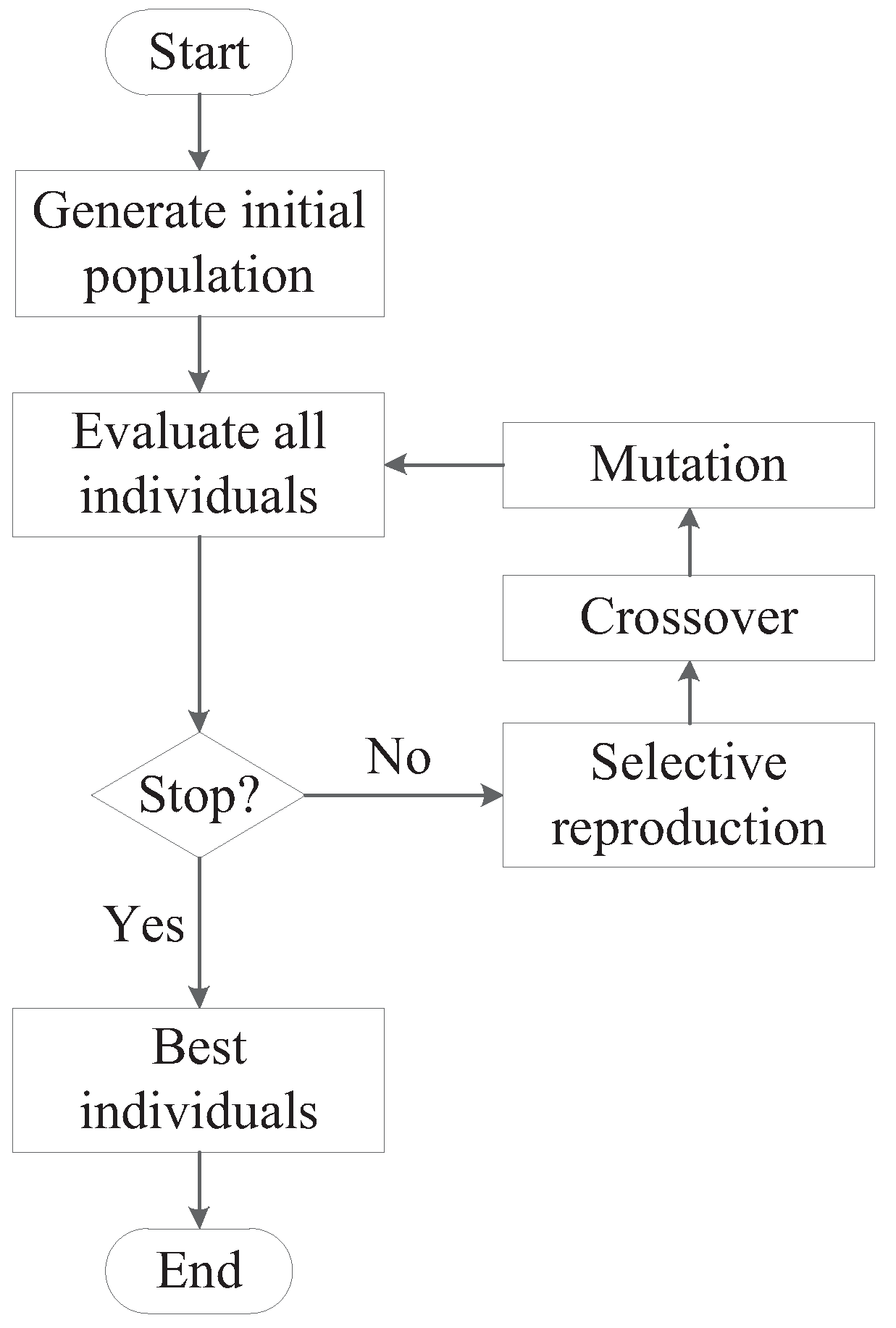
1 η ( K ¯ act , K des ) 0.0005 .
Step 1: 
Generate an initial population
Generate an initial population of individuals randomly or heuristically. Each individual can be represented by a binary string.
Step 2: 
Evaluate all individuals
Compute T p via (29), and evaluate the fitness function f ( T s ) for the individuals of the current population. If T p does not satisfy T p m i n T p T p m a x , set the fitness value as zero.
Step 3: 
Check termination condition
Check if the current population satisfies the termination condition. Stop the iterative procedure if it satisfies, and generate a new population if not.
Step 4: 
Selective reproduction
Select the individuals of the current population (usually with a probability proportional to their relative fitness values) and produce offspring candidates.
Step 5: 
Crossover and mutation
Perform two operators, named crossover and mutation, on the above offspring candidates for producing a new population. Execute Step 3 for the new population.
  • Crossover is the primary genetic operator, which swaps the substrings of two individuals, called parents, before and after a randomly selected crossover point to produce two new individuals, called offsprings.
  • Mutation is essentially an arbitrary modification, which flips bits randomly in a string with a certain probability called the mutation rate.
The diagram of the proposed method is shown in Figure 3.

5. Simulation Examples

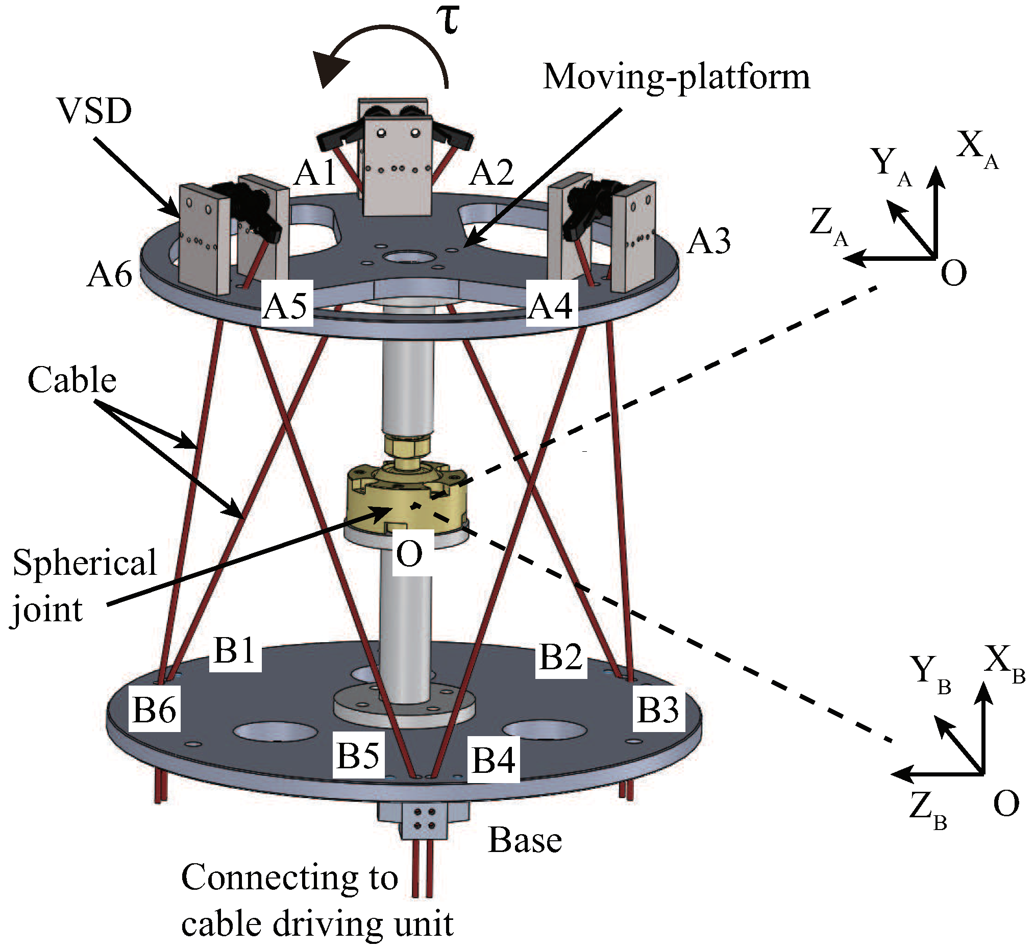
In order to validate the proposed method, a simulation was carried out on a certain 3DJM. As shown in Figure 4, the dimensions of the 3DJM are given by l A = 0.10 [m], l B = 0.13 [m], e A = e B = 0.002 [m] and h A = h B = 0.08 [m].
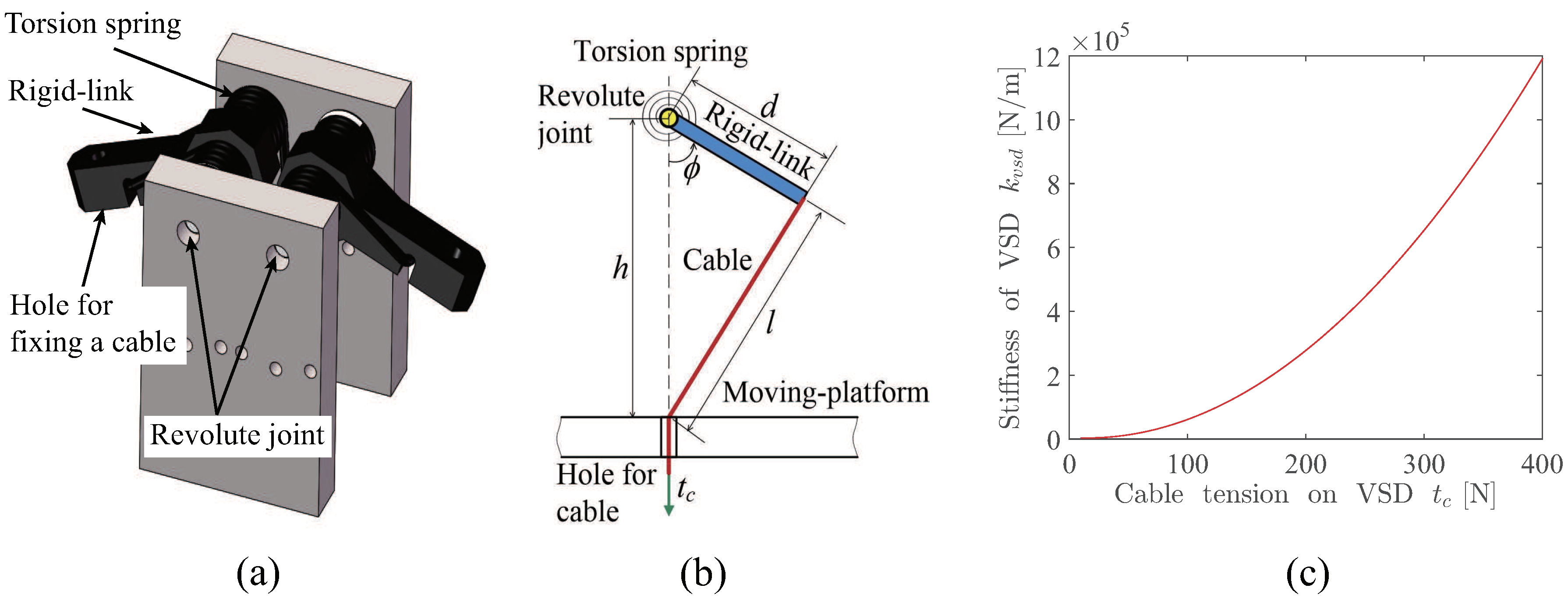
The VSDs were designed to fix onto the moving platform of the 3DJM to extend the range of stiffness variation of each cable. The CAD model of the VSD is shown in Figure 5a. According to the diagram of the VSD, as shown in Figure 5b, the length of the cable in the VSD yields
l = h 2 + d 2 2 h d cos ϕ ,
and the cable tension t c applied on the VSD yields
t c = l k s ( ϕ 0 ϕ ) h d sin ϕ ,
where h R is the height of the revolute joint, d R is the length of the rigid-link, k s R is the stiffness of the spring, ϕ R is the angle of the rigid-link, and ϕ 0 R is the initial value of ϕ . Then the stiffness of the VSD, denoted as k VSD R , can be described by
k VSD = d t c d l = d t c d ϕ / d l d ϕ .
Given the parameters of the designed VSD, i.e., k s = 1.20 Nm/rad, d = 0.018 m, h = 0.03 m, and ϕ 0 = 0.53 rad, the stiffness of the VSD can be approximated by a polynomial expression
k VSD 8.005 t c 2 239.4 t c + 5415 .
The corresponding stiffness–tension curve is shown in Figure 5c. For this 3DJM, the lower limits of the cable tensions are given by
T min = ( 10 , 10 , 10 , 10 , 10 , 10 ) T [ N ] ,
and the upper limits of the cable tensions are given by
T max = ( 400 , 400 , 400 , 400 , 400 , 400 ) T [ N ] .
The simulation examples are implemented for two different desired poses R des 1 and R des2 with different loads, where
R des1 = 0.992 0.060 0.111 0.090 0.952 0.292 0.088 0.300 0.950 , R des2 = 0.950 0.088 0.300 0.111 0.992 0.060 0.292 0.090 0.952 .
For each desired pose, three desired stiffness matrices are given. Thus, the simulation examples can be divided into six sub-cases, as listed in Table 1.
Here, we take Case 1a as an example to perform the proposed method. The other five sub-cases are similar to Case 1a. In Case 1a, the rotation matrix Q is computed according to (24),
Q = 0.159 0.432 0.888 0.727 0.557 0.401 0.668 0.710 0.225 ,
which transforms K des1a to a diagonal matrix E K des1a = diag { 975 , 2937 , 2756 } [Nm/rad]. According to (15), the transpose of the Jacobian matrix J 1 of the 3DJM at the given pose R des1 is computed
S 1 = J 1 T = 0.05 0.02 0.04 0.01 0.03 0.06 0.04 0.04 0 0.05 0.05 0.01 0.01 0.02 0.02 0.01 0.03 0.03 .
The matrix S 1 is divided into two parts as below
S p 1 = 0.05 0.04 0.03 0.04 0 0.05 0.01 0.02 0.03 , S s 1 = 0.02 0.01 0.06 0.04 0.05 0.01 0.02 0.01 0.03 .
The proposed method is implemented to solve the optimization model (34) to find out the cable tension distribution for the desired stiffness K des1a 
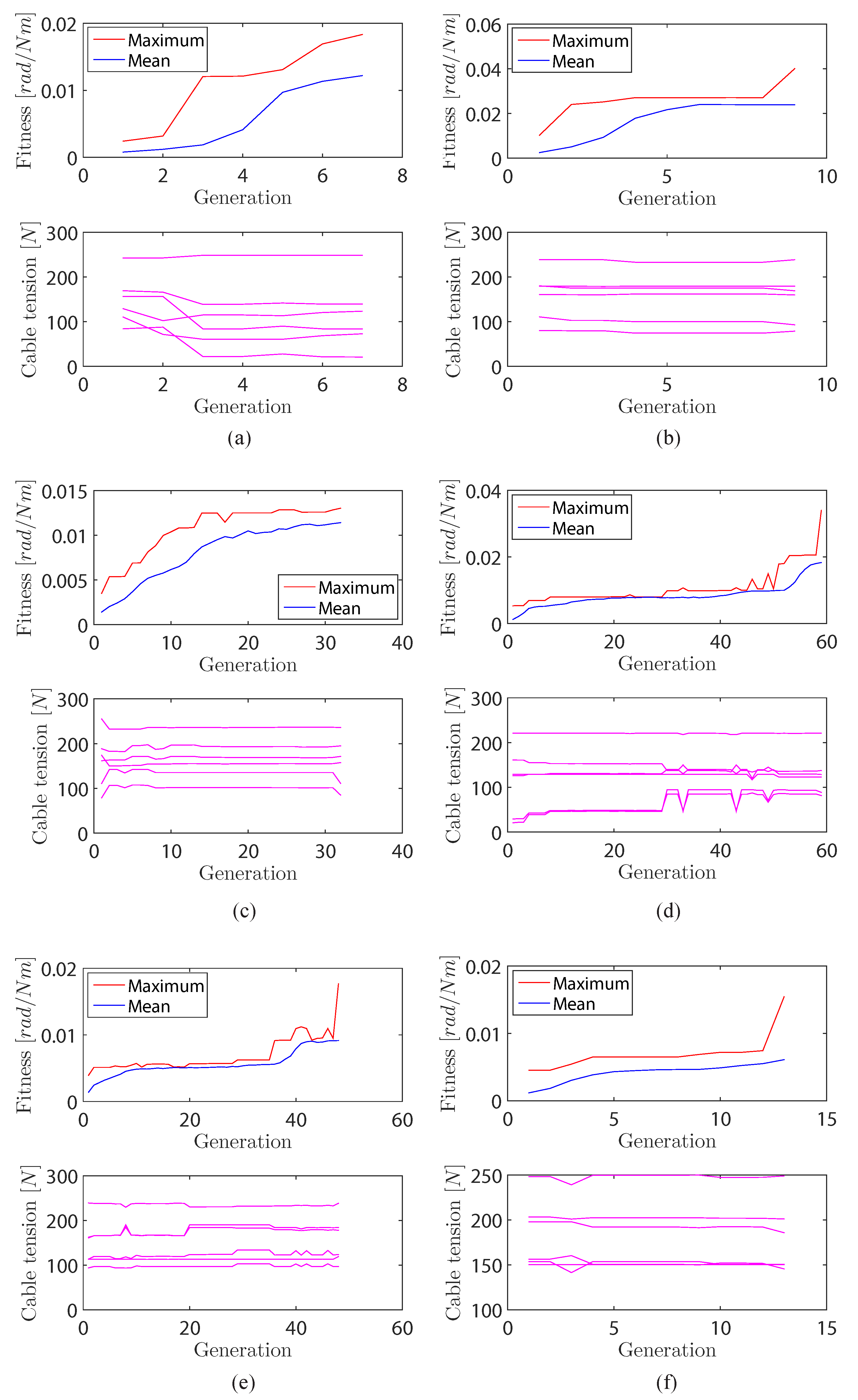
. The iteration curve of the proposed method for Case 1a is shown in Figure 6a, which shows that the optimization process achieves the termination condition within 7 generations and the optimal cable tension distribution for the desired stiffness K des1a is
T opt1a = ( 20.84 , 72.86 , 139.73 , 83.88 , 123.42 , 248.62 ) T [ N ] .
The corresponding actual stiffness K act1a and K ¯ act1a are computed as below
K act1a = 1842.37 339.16 787.59 324.04 388.59 29.52 810.48 61.30 640.20 ,
K ¯ act1a = 1842.37 331.60 799.03 331.60 388.59 45.41 799.03 45.41 640.20 .
According to (36), in Case 1a, η ( K ¯ act1a , K des1a ) = 99.9554 % . It shows that, when the cable tensions achieve T opt1a , the actual stiffness approaches the desired stiffness K des1a .
The results of the simulation for all the six sub-cases are summarized in Table 2 and the corresponding iteration curves of the proposed method are given in Figure 6. The results show that the proposed method can achieve the desired stiffness accurately and efficiently. It is effective for the SCTD problem of the 3DJM.

6. Conclusions

Inspired by the structure of human arms, a modular cable-driven human-like robotic arm (CHRA) was developed for safe human–robot interaction, since it has advantage of flexibility, low moving mass and intrinsic safety. Due to the unilateral driving properties of the cables, the CHRA is redundantly actuated and its stiffness can be adjusted by regulating the cable tensions. The cable tension distribution problem becomes a key element for the stiffness adjustment of the CHRA. Since the trajectory of the 3-DOF joint module (3DJM) of the CHRA is a curve on Lie group SO(3), the stiffness of the 3DJM was evaluated by the covariant derivative of the load to the displacement on SO(3), called an enhanced stiffness model of the 3DJM. In this paper, we focus on analyzing how the cable tension distribution problem oriented the enhanced stiffness of the 3DJM. Since the enhanced stiffness model of the 3DJM is too complicated for solving the cable tensions from the desired stiffness analytically, the SCTD problem was formulated as a nonlinear optimization problem. By analyzing the rank of the Jacobian matrix and the equilibrium equation of the 3DJM, a variable elimination technique was employed to simplify the optimization model. A method based on the genetic algorithm was proposed to solve the optimization model, which only utilized the objective function values. The results of a comprehensive simulation show that the proposed method can solve the cable tension distribution from the desired stiffness accurately and efficiently.

Author Contributions

Conceptualization, K.Y. and G.Y.; supervision, G.Y.; project administration, C.Z. and Y.C.; writing—review and editing, C.C., T.Z. and T.C. All authors have read and agreed to the published version of the manuscript.

Funding

This research is funded by the Public Welfare Technology Research Program of Zhejiang Province, China (Grant number: LGF19E050001), National Natural Science Foundation of China (Grant number:51705510), National-Zhejiang Joint Natural Science Foundation of China (Grant number: U1909215), Institute of robotics and intelligent manufacturing innovation, Chinese Academy of Science (Grant number: C2018005), Ningbo Natural Science Foundation (Grant number: 2019A610114), Open Research Project of the State Key Laboratory of Industrial Control Technology, Zhejiang University, China (Grant number: ICT20048) and Public Welfare Technology Research Program of Zhoushan, China (Grant number: 2019C31067).

Conflicts of Interest

The authors declare no conflict of interest. The funders had no role in the design of the study; in the collection, analyses, or interpretation of data; in the writing of the manuscript, or in the decision to publish the results.

Appendix A. Analysis of the Rank of the Jacobian Matrix of the 3DJM

The transpose of the Jacobian matrix J R 6 × 3 is denoted as S R 3 × 6 , which is represented as below
S = J T = ( a 1 × u 1 , a 2 × u 2 , , a 6 × u 6 ) T .
Assuming the column rank of S satisfies
rank ( S ) < 3 ,
the mixed product of any three column vectors of the matrix S yields
S i · ( S j × S k ) = s i 1 s j 1 s k 1 s i 2 s j 2 s k 2 s i 3 s j 3 s k 3 0 ,
where i , j , k = 1 , 2 , , 6 .
For the 3DJM of the CHRA, the mixed product of any three column vectors of the matrix S can be written as
S i · ( S j × S k ) = ( a i × u i ) · [ ( a j × u j ) × ( a k × u k ) ] = [ a i × ( b i a i ) ] · { [ a j × ( b j a j ) ] × [ a k × ( b k a k ) ] } c i c j c k = ( a i × b i ) · [ ( a j × b j ) × ( a k × b k ) ] c i c j c k 0 ( i , j , k = 1 , 2 , , 6 ) .
In the design of the 3DJM, e A 0 and e B 0 , we have a 1 a 2 , a 3 a 4 , a 5 a 6 , and b 1 b 6 , b 2 b 3 , b 4 b 5 . Then, the following mixed product can be represented as
( a 1 × b 1 ) · [ ( a 2 × b 2 ) × ( a 3 × b 3 ) ] ( a 1 × b 1 ) · [ ( a 1 × b 3 ) × ( a 3 × b 3 ) ] = ( a 1 × b 1 ) · ( μ b 3 ) 0 ,
( a 4 × b 4 ) · [ ( a 2 × b 2 ) × ( a 3 × b 3 ) ] ( a 3 × b 5 ) · [ ( a 1 × b 3 ) × ( a 3 × b 3 ) ] = ( a 3 × b 5 ) · ( μ b 3 ) 0 ,
( a 5 × b 5 ) · [ ( a 2 × b 2 ) × ( a 3 × b 3 ) ] ( a 5 × b 5 ) · [ ( a 1 × b 3 ) × ( a 3 × b 3 ) ] = ( a 5 × b 5 ) · ( μ b 3 ) 0 ,
where μ R and μ 0 .
Equation (A5) shows that vectors b 3 , a 1 and b 1 are in the same plane, (A6) shows that vectors b 3 , a 3 and b 5 are in the same plane, and (A7) shows that vectors b 3 , a 5 and b 5 are in the same plane.
In summary, we have that vectors a 1 , a 3 , a 5 , b 1 , b 3 and b 5 are in the same plane, which is impossible for the 3DJM. The assumption (A2) does not hold, hence
rank ( S ) = 3 ,
i.e.,
rank ( J ) = 3 .

References

  1. Giorelli, M.; Renda, F.; Calisti, M.; Arienti, A.; Laschi, C. Learning the inverse kinetics of an octopus-like manipulator in three-dimensional space. BioInspir. Biomimetics 2015, 10, 035006. [Google Scholar] [CrossRef] [PubMed] [Green Version]
  2. Lau, D.; Oetomo, D.; Halgamuge, S.K. Inverse Dynamics of Multilink Cable-Driven Manipulators with the Consideration of Joint Interaction Forces and Moments. IEEE Trans. Robot. 2015, 31, 479–488. [Google Scholar] [CrossRef] [Green Version]
  3. Lau, D.; Eden, J.; Oetomo, D.; Halgamuge, S.K. Musculoskeletal StaticWorkspace Analysis of the Human Shoulder as a Cable-Driven Robot. IEEE Trans. Mechatron. 2015, 20, 978–984. [Google Scholar] [CrossRef] [Green Version]
  4. Wang, Y.; Song, C.; Zheng, T.; Lau, D.; Yang, K.; Yang, G. Cable Routing Design and Performance Evaluation for Multi-link Cable-Driven Robots with Minimal Number of Actuating Cables. IEEE Access 2019, 7, 135790–135800. [Google Scholar] [CrossRef]
  5. Wang, H.; Zhang, R.; Chen, W.; Wang, X.; Pfeifer, R. A cable-driven soft robot surgical system for cardiothoracic endoscopic surgery-preclinical tests in animals. Surg. Endosc. 2017, 31, 3153–3158. [Google Scholar] [CrossRef] [PubMed]
  6. Li, J.; Lam, J.; Liu, M.; Wang, Z. Compliant Control and Compensation for A Compact Cable-Driven Robotic Manipulator. IEEE Robot. Autom. Lett. 2020, 5, 5417–5424. [Google Scholar] [CrossRef]
  7. Hwang, M.; Thananjeyan, B.; Paradis, S.; Seita, D.; Ichnowski, J.; Fer, D.; Low, T.; Goldberg, K. Efficiently Calibrating Cable-Driven Surgical Robots With RGBD Fiducial Sensing and Recurrent Neural Networks. IEEE Robot. Autom. Lett. 2020, 5, 5937–5944. [Google Scholar] [CrossRef]
  8. Cui, X.; Chen, W.; Jin, X.; Agrawal, S.K. Design of a 7-DOF cable-driven arm exoskeleton (CAREX-7) and a controller for dexterous motion training or assistance. IEEE/ASME Trans. Mechatron. 2017, 22, 161–172. [Google Scholar] [CrossRef]
  9. Kuan, J.; Pasch, K.A.; Herr, H.M. A high-performance cable-drive module for the development of wearable devices. IEEE/ASME Trans. Mechatron. 2018, 23, 1238–1248. [Google Scholar] [CrossRef]
  10. Chen, C.T.; Lien, W.Y.; Chen, C.T.; Twu, M.J.; Wu, Y.C. Dynamic Modeling and Motion Control of a Cable-Driven Robotic Exoskeleton With Pneumatic Artificial Muscle Actuators. IEEE Access 2020, 8, 149796–149807. [Google Scholar] [CrossRef]
  11. Samper-Escudero, J.L.; Gimenez-Fernandez, A.; Sanchez-Uran, M.A.; Frerre, M. A Cable-Driven Exosuit for Upper Limb Flexion Based on Fibres Compliance. IEEE Access 2020, 8, 153297–153310. [Google Scholar] [CrossRef]
  12. Chen, T.; Casas, R.; Lum, P.S. An Elbow Exoskeleton for Upper Limb Rehabilitation With Series Elastic Actuator and Cable-Driven Differential. IEEE Trans. Robot. 2019, 35, 1464–1474. [Google Scholar] [CrossRef] [PubMed]
  13. Dong, X.; Axinte, D.; Palmer, D.; Cobos, S.; Raffles, M.; Rabani, A.; Kell, J. Development of a slender continuum robotic system for on-wing inspection/repair of gas turbine engines. Robot. Comput. Integr. Manuf. 2017, 44, 218–229. [Google Scholar] [CrossRef] [Green Version]
  14. Wang, M.; Palmer, D.; Dong, X.; Alatorre, D.; Axinte, D.; Norton, A. Design and Development of a Slender Dual-Structure Continuum Robot for In-Situ Aeroengine Repair. In Proceedings of the IEEE/RSJ International Conference on Intelligent Robots and Systems (IROS), Madrid, Spain, 1–5 October 2018; pp. 5648–5653. [Google Scholar]
  15. Axinte, D.; Dong, X.; Palmer, D.; Rushworth, A.; Guzman, S.C.; Olarra, A.; Arizaga, I.; Gomez-Acedo, E.; Txoperena, K.; Pfeiffer, K.; et al. MiRoR-Miniaturized Robotic Systems for HolisticIn-SituRepair and Maintenance Works in Restrained and Hazardous Environments. IEEE/ASME Trans. Mechatron. 2018, 23, 978–981. [Google Scholar] [CrossRef]
  16. Campeau-Lecours, A.; Foucault, S.; Laliberte, T.; Mayer-St-Onge, B.; Gosselin, C. A cable-suspended intelligent crane assist device for the intuitive manipulation of large payloads. IEEE/ASME Trans. Mechatron. 2016, 21, 2073–2084. [Google Scholar] [CrossRef] [Green Version]
  17. Dion-Gauvin, P.; Gosselin, C. Dynamic point-to-point trajectory planning of a three-DOF cable-suspended mechanism using the hypocycloid curve. IEEE/ASME Trans. Mechatron. 2018, 23, 1964–1972. [Google Scholar] [CrossRef]
  18. Wang, H.; Kinugawa, J.; Kosuge, K. Exact kinematic modeling and identification of reconfigurable cable-driven robots with dual-pulley cable guiding mechanisms. IEEE/ASME Trans. Mechatron. 2019, 24, 774–784. [Google Scholar] [CrossRef]
  19. Zhang, F.; Shang, W.; Zhang, B.; Cong, S. Design Optimization of Redundantly Actuated Cable-Driven Parallel Robots for Automated Warehouse System. IEEE Access 2020, 8, 56867–56879. [Google Scholar] [CrossRef]
  20. Oh, S.R.; Agrawal, S.K. Cable Suspended Planar Robots with Redundant Cables: Controllers with Positive Tensions. IEEE Trans. Robot. 2005, 21, 457–465. [Google Scholar]
  21. Bruckmann, T.; Pott, A.; Hiller, M. Calculating force distributions for redundantly actuated tendon-based Stewart platforms. In Advances in Robot Kinematics; Springer: Berlin/Heidelberg, Germany, 2006; pp. 403–412. [Google Scholar]
  22. Hassan, M.; Khajepour, A. Optimization of Actuator Forces in Cable-Based Parallel Manipulators Using Convex Analysis. IEEE Trans. Robot. 2008, 24, 736–740. [Google Scholar] [CrossRef]
  23. Borgstrom, P.H.; Jordan, B.L.; Borgstrom, B.J.; Stealey, M.J.; Sukhatme, G.S.; Batalin, M.A.; Kaiser, W.J. NIMS-PL: A Cable-driven Robot with Self-calibration Capabilities. IEEE Trans. Robot. 2009, 25, 1005–1015. [Google Scholar] [CrossRef] [Green Version]
  24. You, X.; Bing, L.; Chen, W.; Yu, S. Tension distribution algorithm of a 7-DOF cable-driven robotic arm based on dynamic minimum pre-tightening force. In Proceedings of the IEEE International Conference on Robotics and Biomimetics (ROBIO), Karon Beach, Thailand, 7–11 December 2011; pp. 715–720. [Google Scholar]
  25. Cote, A.F.; Cardou, P.; Gosselin, C. A tension distribution algorithm for cable-driven parallel robots operating beyond their wrench-feasible workspace. In Proceedings of the International Conference on Control, Automation and Systems, Jeju, Korea, 18–21 October 2017; pp. 68–73. [Google Scholar]
  26. Fang, S.; Franitza, D.; Torlo, M.; Bekes, F.; Hiller, M. Motion Control of a Tendon-BasedParallel Manipulator Using Optimal Tension Distribution. IEEE/ASME Trans. Mechatron. 2004, 9, 561–568. [Google Scholar] [CrossRef]
  27. Gosselin, C. On the Determination of the Force Distribution in Overconstrained Cable-driven Parallel Mechanisms. Meccanica 2011, 46, 3–15. [Google Scholar] [CrossRef]
  28. Lim, W.B.; Song, H.Y.; Yang, G. Optimization of Tension Distribution for Cable-Driven Manipulators Using Tension-Level Index. IEEE/ASME Trans. Mechatron. 2014, 19, 676–683. [Google Scholar] [CrossRef]
  29. Yang, K.; Yang, G.; Chen, S.L.; Wang, Y.; Zhang, C.; Fang, Z.; Zheng, T.; Wang, C. Study on Stiffness-Oriented Cable Tension Distribution for a Symmetrical Cable-Driven Mechanism. Symmetry 2019, 11, 1158. [Google Scholar] [CrossRef] [Green Version]
  30. Yang, K.; Yang, G.; Chen, S.L.; Wang, Y.; Zheng, T.; Fang, Z.; Wang, C. Enhanced Stiffness Modeling and Identification Method for a Cable-driven Spherical Joint Module. IEEE Access 2019, 7, 137875–137886. [Google Scholar] [CrossRef]
  31. Murray, R.N.; Li, Z.; Sastry, S. A Mathematical Introduction to Robotics Manipulation; CRC Press: Boca Raton, FL, USA, 1994. [Google Scholar]
  32. Lee, J.M. Introduction to Riemannian Manifolds; Springer: Berlin/Heidelberg, Germany, 2018. [Google Scholar]
  33. Zefran, M.; Kumar, V. A geometric approach to the study of the Cartesian stiffness matrix. J. Mech. Des. 2002, 124, 30–38. [Google Scholar] [CrossRef]
  34. Golub, G.H.; Charles, F.V.L. Matrix Computations; The Johns Hopkins University Press: Baltimore, MD, USA, 1985. [Google Scholar]
  35. Nelder, J.A.; Mead, R. A simplex method for function minimization. Comput. J. 1965, 7, 308–313. [Google Scholar] [CrossRef]
  36. Affenzeller, M.; Winkler, S.; Wagner, S.; Beham, A. Genetic Algorithms and Genetic Programming-Modern Concepts and Practical Applications; CRC Press: Boca Raton, FL, USA, 2009. [Google Scholar]
Figure 1. Concept design of the modular cable-driven human-like robotic arm: (a) structure of a human arm, (b) structure of the cable-driven human-like robotic arm (CHRA).
Applsci 10 08871 g001
Figure 2. Concept design of the 3-DOF joint module (3DJM).
Applsci 10 08871 g002
Figure 3. Diagram of the proposed method for the stiffness-oriented cable tension distribution problem of the 3DJM.
Applsci 10 08871 g003
Figure 4. CAD model of the 3DJM.
Applsci 10 08871 g004
Figure 5. variable-stiffness device (VSD) for simulation: (a) CAD model of the VSD, (b) diagram of the VSD, (c) stiffness–tension curve of the VSD.
Applsci 10 08871 g005
Figure 6. Iteration curves of the proposed method for the six sub-cases: (a) Case 1a, (b) Case 1b, (c) Case 1c, (d) Case 2a, (e) Case 2b, (f) Case 2c.
Applsci 10 08871 g006
Table 1. Six sub-cases of the simulation with different desired poses, applied loads and desired stiffness matrices.
CasePose R des Load τ [Nm]Desired Stiffness K des [Nm/rad]
Case 1a R des1 τ 1a = 11.62 8.09 4.05 K des1a = 1806.79 323.63 765.79 323.63 443.92 49.61 765.79 49.61 634.78
Case 1b R des1 τ 1b = 9.26 11.39 4.55 K des1b = 1131.24 160.46 62.27 160.46 1918.78 134.28 62.27 134.28 588.78
Case 1c R des1 τ 1c = 7.24 6.60 2.72 K des1c = 1600.13 353.41 320.28 353.41 1687.70 244.90 320.28 244.90 477.74
Case 2a R des2 τ 2a = 2.95 8.05 2.08 K des2a = 1302.42 140.27 518.72 140.27 617.78 147.18 518.72 147.18 503.89
Case 2b R des2 τ 2b = 7.64 9.56 5.90 K des2b = 1670.44 180.42 499.26 180.42 1226.99 350.38 499.26 350.38 676.84
Case 2c R des2 τ 2c = 3.70 14.72 2.58 K des2c = 1563.55 298.57 15.13 298.57 2395.40 280.72 15.13 280.72 687.41
Table 2. Results of the simulation for the six sub-cases.
CaseDesired Stiffness K des Actual Stiffness K ¯ act [Nm/rad] η ( K ¯ act , K des )
Case 1a K des1a K ¯ act1a = 1842.37 339.16 787.59 324.04 388.59 29.52 810.48 61.30 640.20 99.9554%
Case 1b K des1b K ¯ act1b = 1115.72 171.67 42.79 155.02 1900.10 124.34 75.13 148.55 583.72 99.9991%
Case 1c K des1c K ¯ act1a = 1593.57 345.80 335.65 335.65 357.47 1610.93 264.71 353.79 466.67 99.9584%
Case 2a K des2a K ¯ act2a = 1316.56 106.95 503.13 109.93 636.37 137.96 524.24 128.03 504.65 99.9500%
Case 2b K des2b K ¯ act2b = 1679.74 187.54 464.93 208.97 1276.25 366.06 489.22 343.72 676.79 99.9697%
Case 2c K des2c K ¯ act2c = 1627.92 283.30 33.88 295.86 2390.02 270.50 73.42 282.15 710.07 99.9629%
Publisher’s Note: MDPI stays neutral with regard to jurisdictional claims in published maps and institutional affiliations.

