Abstract
In this work, we present a panoramic 3D stereo reconstruction system composed of two catadioptric cameras. Each one consists of a CCD camera and a parabolic convex mirror that allows the acquisition of catadioptric images. We describe the calibration approach and propose the improvement of existing deep feature matching methods with epipolar constraints. We show that the improved matching algorithm covers more of the scene than classic feature detectors, yielding broader and denser reconstructions for outdoor environments. Our system can also generate accurate measurements in the wild without large amounts of data used in deep learning-based systems. We demonstrate the system’s feasibility and effectiveness as a practical stereo sensor with real experiments in indoor and outdoor environments.
1. Introduction
Conventional stereoscopic reconstruction systems based on perspective cameras have a limited field-of-view that restricts them in applications that involve wide areas such as large-scale reconstruction or self-driving cars. To compensate for the narrow field-of-view, these systems acquire multiple images and combine them to cover the desired scene [1]. A different way to increase the field-of-view is to use fish-eye lenses [2] or mirrors in conjunction with lenses to constitute a panoramic catadioptric system [3,4].
Catadioptric omnidirectional stereo vision can be achieved using one camera with multiple mirrors [5,6]; two cameras and a single mirror [7] or two cameras and two mirrors [8]. The common types of mirrors used are hyperbolic double mirrors [9], multiple conic mirrors [10,11], multiple parabolic mirrors [12], concave lens with a convex mirrors [13,14], multi-planar mirrors [15], and mirror pyramids [16]. The large field-of-view of these systems makes them useful in applications such as driver assistance tasks [17,18], unmanned vehicle aerial navigation [19,20,21], visual odometry [22], and 3D reconstruction for metrology applications [23,24].
To perform 3D reconstruction with a stereo system, we need to find matching points on the set of cameras. Typically, there are two methods for matching image pairs in passive stereo systems: dense methods based on finding a disparity map by pixel-wise comparison of rectified images along the image rows, and sparse methods using matching features based on pixel region descriptors.
One challenge of the dense methods with panoramic images is that the rectified images are heavily distorted, and their appearance depends on the relative configuration of the two cameras. Therefore, many pixels are interpolated in some image regions, influencing pixel mapping precision and 3D reconstruction. A limitation of dense omnidirectional stereo matching is the running time making it not suitable for real-time applications [25].
On the other hand, sparse methods with panoramic images provide a confined number of matching features for triangulation [26,27] due to the reduced spatial resolution, wasted image-plane pixels, and exposure control [28]. Due to this, it is a common practice to manually select matching points for calibration or to validate the measurements [5,29]. Another prevalent limitation of these systems is the validation in indoor environments only. For example, Mao et al. [26] present a reconstruction algorithm for multiple spherical images; they use a combination of manually selected points and SIFT matching to estimate the fundamental matrix for each image pairs and present sparse reconstruction results in indoor environments. Fiala et al. [5], present a bi-lobed panoramic sensor with the matching features detected using the Panoramic Hough Transform. The results show sparse points of scene polygons in indoor environments. The work presented by [29] similar to our research proposal, shows a sensor with the same amount of components but with the use of hyperbolic mirrors. The 3D reconstruction was done on manually selected points to avoid possible errors due to an automatic matching. To validate the method, they selected four corners of the ceiling to compute the size of the room with an estimated error between 1 and 6 cm. Zhou et al. [30] propose an omnidirectional stereo vision sensor composed of one CCD camera and two pyramid mirrors. To evaluate the performance of the proposed sensor, they tested a calibration plane. Although this sensor cannot accomplish a whole panoramic view, it nevertheless provides a useful vision measurement approach for indoor scenes. Jang et al. [31] propose a catadioptric stereo camera system that uses a single camera and a single lens with conic mirrors. Stereo matching was conducted with a window-based correlation search. The disparity map and the depth map show good reconstruction accuracy indoors except for ambiguous regions like repetitive wall patterns where the intensity-based matching does not work. Ragot et al. [32] propose a dense matching algorithm based on interpolation of sparse points. The matchings points are processed during calibration, and results are stored in Look-Up Tables. The reconstruction algorithms are validated on synthetic images and real indoor images. Chen et al. [4] present a catadioptric multi-stereo system composed of a single camera and five spherical mirrors. They implemented a dense stereo matching and multi point cloud fusion. The results presented in indoor scenes improved between 15% to 30% when combining the stereo results.
Alternatively, deep learning techniques have recently obtained remarkable results in estimating depth from a single perspective image in indoor and outdoor environments. Depth estimation can be defined as a pixel-level regression, and the model architectures usually use Convolutional Neural Networks (CNNs) architectures. Xu et al. [33] proposed predicting depth maps from RGB inputs in a multi-scale framework combining CNNs with Conditional Random Fields (CRF). Later in [34] they propose a multi-task architecture called PAD-Net capable of simultaneously perform depth estimation and scene parsing. Fu et al. [35] introduced a depth estimation network that uses dilated convolutions and a full-image encoder to directly obtain a high-resolution depth map and improve the training time through depth discretization and the use of ordinal regression loss. More related to our work is the one from Won et al. [36], where an end-to-end deep learning model estimates depth from multiple fisheye cameras. Their network can learn global context information and reconstructs accurate omnidirectional depth estimates. However, all these methods require large training sets of RGB-depth pairs, which can be expensive to obtain, and the quality of the results is limited by the data used for training.
Deep Learning techniques have also been applied in feature matching, and optical flow applications [37,38]. Sarlin et al. [39] proposed a graph neural network along with a context aggregation mechanism based on attention to allow their model to reason about the 3D information and the feature assignments. However, the performance is bounded by the training data used and the augmentations performed during training.
To combine the best of both approaches (panoramic imaging and Deep Learning), in this work, we present a stereo catadioptric system that uses a deep learning-inspired feature matching algorithm called DeepMatching [40] augmented with stereo epipolar constraints. With this, our system can produce wide field-of-view 3D reconstructions in indoor and outdoor scenes without the need of specific training data.
The main contributions of this work are twofold. First, we propose a catadioptric stereo system capable of generating semi-dense reconstructions using deep learning matching methods such as DeepMatching [40] with stereo epipolar constraints. Second, the system can produce 3D reconstructions in indoor or outdoor environments at higher framerate than dense methods without new training data.
2. Catadioptric Vision System
This section presents the catadioptric vision system’s experimental arrangement, which consists of two omnidirectional cameras, including a CCD camera and a parabolic mirror.
Experimental Setup
Figure 1 shows a schematic overview of the experimental setup for the proposed panoramic 3D reconstruction system, which consists of two catadioptric cameras; an upper camera and a lower camera, each composed of a 0–360 parabolic mirror and a Marlin F-080 CCD camera on a back-to-back configuration.
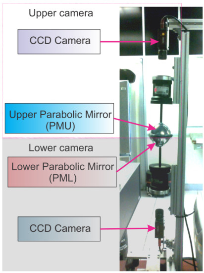
Figure 1.
Panoramic 3D reconstruction system formed by two catadioptric cameras (upper camera and lower camera), each composed by a parabolic mirror and a Marlin F-080c camera.
We assembled the catadioptric cameras to capture the full environment that is reflected in the mirrors. For this purpose, we aligned a mirror with the lower CCD camera to compose the lower parabolic mirror (PML). Then we placed another mirror back-to-back with PML aligned with the upper CCD camera to produce the upper parabolic mirror (PMU). Using a chessboard calibration pattern, we calibrate both catadioptric cameras obtaining their intrinsic and extrinsic parameters, as explained in the next section.
3. Methodology
This section presents the methodology to perform 3D reconstruction of an object or scene using the proposed catadioptric stereo system. Section 3.1 describes the calibration procedure, Section 3.2 explains the epipolar geometry for panoramic cameras, and Section 3.3 describes the stereo reconstruction.
3.1. Catadioptric Camera Calibration
To perform 3D reconstructions with metric dimensions, it is necessary to know the cameras’ intrinsic parameters, such as the focal length, optical center, mirror curvature, and extrinsic parameters composed by the rotation and translation between them. These parameters are obtained with the camera calibration. This section briefly describes the process to calibrate the catadioptric stereo vision system based on the work presented in [41].
To calibrate the catadioptric cameras, we used the geometric model proposed in [42]; this model uses a checkerboard pattern (shown in Figure 2a) to obtain the intrinsic parameters of each camera and the extrinsic parameters between the reference system of the cameras and that of the pattern. The pixel coordinates of a point in the image are represented by . Equation (1) shows the relation between a 3D point in the mirror and a 2D point in the image.

Figure 2.
Calibration pattern. (a) Chessboard pattern (b) Images of the pattern using the upper camera. (c) Images of the pattern using the lower camera.
Since the mirror is rotationally symmetric, the function only depends on the distance leading to Equation (2).
where is a fourth degree polynomial that defines the curvature of the parabolic mirror:
the coefficients correspond to the intrinsic parameters of the mirror.
3.2. Epipolar Geometry for Panoramic Cameras
Epipolar geometry describes the relationship between positions of corresponding points in a pair of images acquired by different cameras [41,43,44]. Given a feature point in one image, its matching view in the other image must lie along the corresponding epipolar curve. This fact is known as the epipolar constraint. Once we know the stereo system’s epipolar geometry, the epipolar constraint allows us to reject feature points that could otherwise lead to incorrect correspondences.
In our system, the images are acquired by the catadioptric system formed by the upper camera-mirror (PMU) and the lower camera-mirror (PML), as seen in Figure 3. The projections of a 3D point over the mirrors PMU and PML are denoted by and respectively. The coplanarity of the vectors , , is expressed by Equation (4)
where × corresponds to the cross product and R and are the rotation matrix and translation vector between the upper and lower mirrors. The coplanarity restriction is simplified in Equation (5)
where:
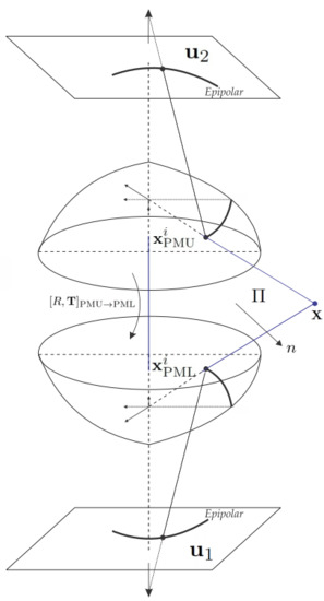
Figure 3.
Epipolar geometry between two catadioptric cameras with parabolic mirrors. R is the rotation matrix and is the translation vector, between the upper and lower mirrors (PMU→PML) expressed as a skew symmetric matrix. is the epipolar plane.
For every point in the catadioptric image, an epipolar conic is uniquely assigned to the other image , the search space between corresponding points is limited by Equation (8).
In the general case, the matrix is a non-linear function of the essential matrix E, the points , and the calibration parameters of the catadioptric camera.
The vector defines the epipolar plane . Equation (9) describes the vector normal to the plane in the camera coordinates system.
The normal vector can be expressed in the second camera coordinate system using the essential matrix as follows:
Then Equation (10) is represented as:
The plane equation described in the second camera coordinate system is given by Equation (12).
The derivation of from Equation (8) based on a parabolic mirror, z is substituted into Equation (12) resulting in Equation (13) that allows the calculation of the epipolar conics for this type of mirror:
where is the mirror parameter and are the components of the normal vector computed in Equation (10).
3.3. Stereo Reconstruction
Once we have the system calibrated, the next step is to acquire images and reconstruct a scene using the following procedure (see Figure 4):
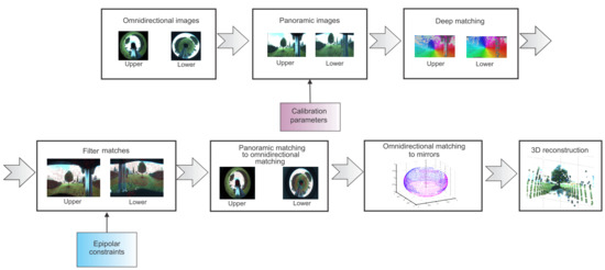
Figure 4.
Panoramic 3D reconstruction (best seen in color). The procedure is the following: (1) Capture images from the catadioptric camera system, (2) unwrap the omnidirectional images to obtain panoramic images (3) to search for feature matches and (4) filter the matches using epipolar constraints. (5) Convert features back to catadioptric image coordinates and (6) to mirror coordinates. (7) Perform 3D reconstruction.
- 1
- Capture one image of the environment from each camera of the calibrated system.
- 2
- Transform the catadioptric images to panoramic images using Algorithm 1.
- 3
- Extract the features and descriptors from the panoramic images using a feature point detector such as SIFT, SURF, KAZE, a corner detector such as Harris, or more advanced feature detectors such as DeepMatching [40], CPM [45], or SuperGlue [39]. Match the points between the upper and lower camera features as described in Section 3.3.1.
- 4
- Filter the wrong matches using epipolar constraints as described in Section 3.2.
- 5
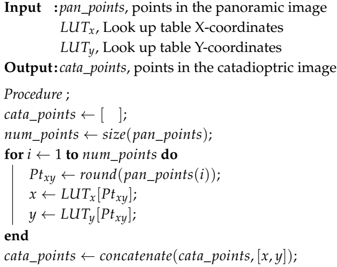
- Map the matching points coordinates from panoramic back to catadioptric images coordinates, using Algorithm 2.
- 6
- Transform the catadioptric image points to the corresponding mirror PMU and PML.
- 7
- Obtain the 3D reconstruction by triangulating the mirror points points using Equation (15) describe in Section 3.3.2.
| Algorithm 1:Transforming catadioptric images to panoramic images |
| Input: img_cat, catadioptric image , , optical center Output: img_pan, panoramic image , Look up table X-coordinates , Look up table Y-coordinates Procedure; ; ; ; to ; to ; ; ; ; ; ; |
| Algorithm 2:Mapping between catadioptric to panoramic images |
 |
3.3.1. Feature Detection and Matching
A feature point in an image is a small patch with enough information to be found in another image. Feature points can be corners, which are image patches with significant changes in both directions and are rotation-invariant [46,47]. They can be keypoints that encode texture information in vectors called descriptors, which besides being rotation-invariant, are also scale-invariant [48,49,50,51,52]. Additionally, they can be Deep Learning-based features that can also be invariant to repetitive textures and non-rigid deformations [39,40].
Feature matching entails finding the same feature point in both images, for this, we compared corner detectors such as Harris [46] and Shi-Tomasi [47] along with feature point detectors such SIFT [48], SURF [49], BRISK [50], FAST [51], KAZE [52], a state-of-the-art Deep Learning method called SuperGlue [39] and DeepMatching [40]. In the case of a corner detector, we use epipolar geometry described in Section 3.2 to reduce the search along the epipolar curve and match the points using image-patch correlation.
For the case of a feature point detector, we compute the pairwise distance between the descriptor vectors. Two descriptor vectors match when the distance between them is less than a defined threshold t; for BRISK and for SIFT, SURF, KAZE, and FAST. For the case of SuperGlue, we used the outdoor trained model provided by the authors for the outdoor scene and the indoor trained model for the indoor scene. For DeepMatching, after finding the matches using the original implementation, we filter out the wrong matches using epipolar constraints. For this, we measure the Euclidean distance to the epipolar curve and keep the corresponding point in the other image if it lies d pixels from the epipolar. Figure 5c shows a selected feature as a red mark in the upper panoramic image, and Figure 5d shows the matched point in the lower panoramic image as a red mark along with the epipolar line through which the point should lie.
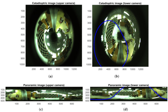
Figure 5.
Feature point and epipolar curve (best seen in color). (a) Feature point (red mark) in the upper catadioptric image, (b) Feature point (red mark) and epipolar curve in the lower catadioptric image, (c) Feature point (red mark) in the upper panoramic image, (d) Feature point (red mark) and epipolar curve in the lower panoramic image.
3.3.2. 3D Reconstruction
Once we have the feature points between the two catadioptric cameras, we convert those coordinates to mirror coordinates to perform the 3D reconstruction.
Given point pairs and on the mirrors surfaces and the coordinates of a point , we obtained Equation (14) [41,43].
From the distance between two points and , we determined the coordinates of a point using Equation (15).
4. Results
This section presents the results for the system calibration, catadioptric epipolar geometry, feature matching, and 3D reconstruction.
4.1. Calibration Results
Table 1 shows the intrinsic parameters of the upper and lower cameras, respectively. As described in Section 3.1, are the coefficients of a fourth degree polynomial that defines the curvature of the parabolic mirror representing the intrinsic parameters of the mirror. and define the optical center of the catadioptric cameras with a resolution of .

Table 1.
Intrinsic parameters of upper and lower camera.
We obtain the extrinsic parameters of the upper and lower catadioptric cameras with respect to each calibration plane (Figure 2a). That is, six extrinsic parameters (rotation and translation) for each of the 32 images acquired during calibration. The calibration errors of each catadioptric camera are shown in Table 2 which are inside the ranges of typical panoramic cameras [53].

Table 2.
Calibration error on the catadioptric camera.
4.2. Epipolar Geometry Results
In this section, we show how the epipolar curves can be used to filter wrong matching points. Figure 5a shows a feature point (red mark) on the upper catadioptric image, and Figure 5b shows the corresponding point on the lower catadioptric image along with the epipolar curve shown in blue. Figure 5c,d show the same information but for the unwrapped panoramic images. For a corresponding point in the lower camera to be correct, it must lie along the epipolar curve, as shown in the images.
4.3. Features Matching Results
We compared the feature detection and matching using multiple methods. Table 3 shows the number of feature matches found with each method in descending order as well as the running time. We use MATLAB 2019b built-in functions for all the methods except SIFT, DeepMatching, and SuperGlue. For SIFT, we use the Machine Vision Toolbox from [54], and for DeepMatching and SuperGlue we use the original implementations [55,56]. For these last two methods, we report the inference time on a CPU Intel Xeon ES-1630 at 3.7 GHz and on a GPU GTX1080. Although these two methods are slow on CPU due to the computationally expensive nature of deep neural networks, the parallel GPU implementation can achieve running times comparable to the other CPU-based methods.

Table 3.
Number of matches and running times obtained with each method. For the Deep learning-based methods, we also report the running times obtained in a GTX 1080.
Figure 6 and Figure 7 show the feature matches for the first six methods shown in Table 3. From these images, we can see that DeepMatching has a significantly broader coverage and density at the expense of higher computational cost. The second best feature detector in terms of the number of features was the Harris corner detector; however, we can see that the features cover only the trees’ borders but not the entire image. KAZE and SuperGlue matches have more image coverage than Harris, but the features are sparse compared to DeepMatching.
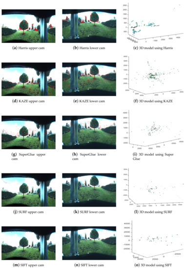
Figure 6.
Feature matching points on the upper and lower cameras and 3D reconstruction for each comparing method.
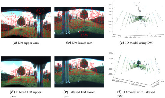
Figure 7.
DeepMatching features and reconstruction. (a,b) show the original DeepMatching on the upper and lower camera, respectively. (c) shows the 3D reconstruction using the original DeepMatching. (d,e) show the filtered DeepMatching using epipolar constraints with on the upper and lower cameras. (f) shows the 3D reconstruction using filtered DeepMatching.
As described in Section 3.3.1, we filtered the DeepMatching results using epipolar constraints by keeping the matches whose distance from the epipolar curve is less than a defined threshold d. Figure 8 shows the number of DeepMatching features obtained with different filtering levels. The more we increase d, the more matches we get, but also, the more error we are allowing in the reconstruction. Empirically, we found that a value of d between 20 and 30 pixels from the epipolar curve gives the best compromise between features and features’ quantity and quality. The effects of d in the reconstruction are described in the next section.
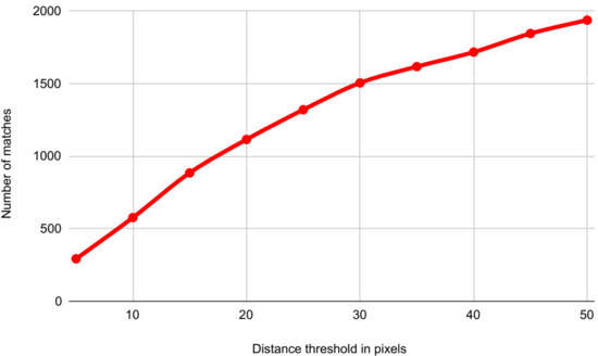
Figure 8.
Amount of DeepMatching features obtained with different levels of filtering. The more we increase the distance threshold, the more matches we get, but also, the more error we are allowing in the reconstruction.
4.4. 3D Reconstruction Results
Once we have the matching points in both catadioptric cameras, the next step is to transform those points into the mirrors. Figure 9a shows the Harris corners (which was the runner-up method in terms of the number of features) on the upper parabolic mirror (PMU) and the lower panoramic mirror (PML). Similarly, Figure 9b shows the DeepMatching points on each of the mirrors. As described in Section 4.3, DeepMatching provides broader coverage and density than all the other methods (see Figure 6 and Figure 7) shown in Table 3 resulting in a more well-rounded reconstruction.
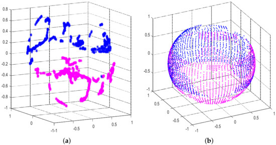
Figure 9.
Matching points in the panoramic mirrors (best seen in color). Pink points denote the features in the panoramic upper mirror PMU, and blue points are the features on the panoramic lower mirror PML. (a) Shows Harris corners on the mirrors, and (b) shows the DeepMatching points on the mirrors.
The third columns of Figure 6 and Figure 7 show the reconstruction of an outdoor scenario with features obtained with the methods presented in Table 3. Figure 6a–c show the Harris corners matches and the reconstruction, Figure 6d–f using KAZE, Figure 6g–i applying SuperGlue, Figure 6j–l employing SURF, Figure 6m–o with SIFT, and Figure 7 with DeepMatching.
For this challenging outdoor environment, we see that the reconstructions generated with the feature matches from all these methods are poor due to the lack of feature density and coverage except for the DeepMatching method, where the features can cover most of the image as shown in Figure 7.
Although DeepMatching returns many feature matches, not all of them are correct. To fix this, we use epipolar constraints as described in Section 3.2. Figure 7a,b show the unfiltered DeepMatching results along with the 3D reconstruction in Figure 7c. Figure 7d,e show the DeepMatching results filtered with pixels. Figure 7f shows the reconstruction with these filtered features points.
Figure 10 shows the point clouds reconstructed using the Deep features matches with the different filtering levels. As the images show, when we relax the filter (when d is larger), we get more features but also more errors in the background.

Figure 10.
3D reconstruction using DeepMatching. Figures (a–c) show the reconstruction with features filtered at , , and respectively.
To quantify the reconstruction error, we reconstruct an object with known dimensions, in this case a rectangular pattern of size 50 cm × 230 cm. Figure 11 shows the results obtained with DeepMatching. Figure 11a,b show the unfiltered DeepMatching features and Figure 11c shows the 3D reconstruction. Figure 11d,e show the filtered matches with and Figure 11f shows the 3D reconstruction. From Figure 11 we see that the filtering of the features using epipolar constraints produces a cleaner reconstruction without compromising the density.
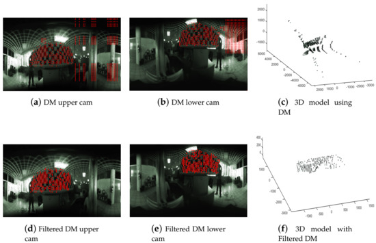
Figure 11.
DeepMatching and filtered DeepMatching for 3D reconstruction of a known pattern.
Using the rectangular pattern with known dimensions, we calculate the reconstruction’s error at the center of the pattern and the extremes. At the right extreme, the error correlates with a larger distortion on the periphery of the mirror. Table 4 shows the mean reconstruction error in millimeters and the standard deviation.

Table 4.
Reconstruction error in millimeters.
To evaluate the qualitative results of the 3D reconstructions, we reconstructed three more objects shown in Figure 12. A squared box, a hat, and a clay pot. For the squared box shown in Figure 12a, we computed the angles between normal vectors of adjacent planes compared with . The results are shown in Table 5. In this table, we compared the angle errors with [4] achieving slightly better results with one stereo pair.
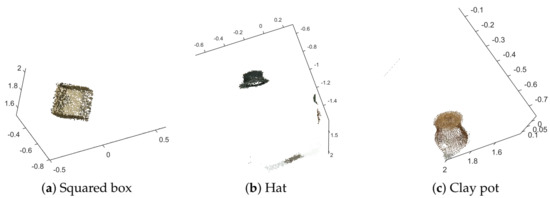
Figure 12.
Qualitative reconstructions results using filtered DeepMatching. (a) Shows the reconstruction of a squared box, (b) shows the reconstruction of a hat, and (c) shows the reconstruction of a clay pot.

Table 5.
Angle errors of the squared box.
5. Conclusions
We introduced the development of a stereo catadioptric 3D reconstruction system capable of generating semi-dense reconstructions based on epipolar constrained DeepMatching. The proposed method generates accurate 3D reconstructions for indoor and outdoor environments with significantly more matches than sparse methods, producing broader and denser 3D reconstructions and gracefully removing incorrect correspondences provided by the DeepMatching algorithm. Our system’s current limitations in terms of hardware are its large size and fragility, making it unsuitable for real-life situations. In terms of the method, although DeepMatching provides significantly more feature points than corner or feature-point detectors, it is still relatively sparse compared to dense 3D reconstruction deep learning techniques at the expense of faster and more accurate measurements. In future work, we plan to increase the reconstruction’s density by combining the current approach with dense 3D reconstruction methods and improving the system’s size and robustness.
Author Contributions
Conceptualization, D.M.C.-E. and J.T.; Methodology, D.M.C.-E.; Resources, D.M.C.-E., J.T., J.A.R.-G., A.R.-P.; Software, D.M.C.-E., J.T., J.A.R.-G., A.R.-P.; Writing—original draft, D.M.C.-E. and J.T.; Writing—review and editing, D.M.C.-E., J.T., J.A.R.-G., A.R.-P. All authors have read and agreed to the published version of the manuscript.
Funding
This research received no external funding.
Acknowledgments
The authors wish to acknowledge the support for this work by the Consejo Nacional de Ciencia y Tecnología (CONACYT) through Sistema Nacional de Investigadores (SNI). We also want to thank CICATA-IPN, Queretaro for providing the facilities and support during the development of this project.
Conflicts of Interest
The authors declare no conflict of interest.
References
- Jiang, W.; Okutomi, M.; Sugimoto, S. Panoramic 3D reconstruction using rotational stereo camera with simple epipolar constraints. In Proceedings of the 2006 IEEE Computer Society Conference on Computer Vision and Pattern Recognition (CVPR’06), New York, NY, USA, 17–22 June 2006; Volume 1, pp. 371–378. [Google Scholar]
- Deng, X.; Wu, F.; Wu, Y.; Wan, C. Automatic spherical panorama generation with two fisheye images. In Proceedings of the 2008 7th World Congress on Intelligent Control and Automation, Chongqing, China, 25–27 June 2008; pp. 5955–5959. [Google Scholar]
- Sagawa, R.; Kurita, N.; Echigo, T.; Yagi, Y. Compound catadioptric stereo sensor for omnidirectional object detection. In Proceedings of the 2004 IEEE/RSJ International Conference on Intelligent Robots and Systems (IROS)(IEEE Cat. No. 04CH37566), Sendai, Japan, 28 September–2 October 2004; Volume 3, pp. 2612–2617. [Google Scholar]
- Chen, S.; Xiang, Z.; Zou, N.; Chen, Y.; Qiao, C. Multi-stereo 3D reconstruction with a single-camera multi-mirror catadioptric system. Meas. Sci. Technol. 2019, 31, 015102. [Google Scholar] [CrossRef]
- Fiala, M.; Basu, A. Panoramic stereo reconstruction using non-SVP optics. Comput. Vis. Image Underst. 2005, 98, 363–397. [Google Scholar] [CrossRef]
- Jaramillo, C.; Valenti, R.G.; Xiao, J. GUMS: A generalized unified model for stereo omnidirectional vision (demonstrated via a folded catadioptric system). In Proceedings of the 2016 IEEE/RSJ International Conference on Intelligent Robots and Systems (IROS), Daejeon, Korea, 9–14 October 2016; pp. 2528–2533. [Google Scholar]
- Lin, S.S.; Bajcsy, R. High resolution catadioptric omni-directional stereo sensor for robot vision. In Proceedings of the 2003 IEEE International Conference on Robotics and Automation (Cat. No. 03CH37422), Taipei, Taiwan, 14–19 September 2003; Volume 2, pp. 1694–1699. [Google Scholar]
- Ragot, N.; Ertaud, J.; Savatier, X.; Mazari, B. Calibration of a panoramic stereovision sensor: Analytical vs. interpolation-based methods. In Proceedings of the Iecon 2006-32nd Annual Conference on Ieee Industrial Electronics, Paris, France, 6–10 November 2006; pp. 4130–4135. [Google Scholar]
- Cabral, E.L.; De Souza, J.; Hunold, M.C. Omnidirectional stereo vision with a hyperbolic double lobed mirror. In Proceedings of the 17th International Conference on Pattern Recognition, Cambridge, UK, 26 August 2004; Volume 1, pp. 1–9. [Google Scholar]
- Jang, G.; Kim, S.; Kweon, I. Single-camera panoramic stereo system with single-viewpoint optics. Opt. Lett. 2006, 31, 41–43. [Google Scholar] [CrossRef]
- Su, L.; Luo, C.; Zhu, F. Obtaining obstacle information by an omnidirectional stereo vision system. In Proceedings of the 2006 IEEE International Conference on Information Acquisition, Weihai, China, 20–23 August 2006; pp. 48–52. [Google Scholar]
- Caron, G.; Marchand, E.; Mouaddib, E.M. 3D model based pose estimation for omnidirectional stereovision. In Proceedings of the 2009 IEEE/RSJ International Conference on Intelligent Robots and Systems, St. Louis, MO, USA, 10–15 October 2009; pp. 5228–5233. [Google Scholar]
- Yi, S.; Ahuja, N. An omnidirectional stereo vision system using a single camera. In Proceedings of the 18th International Conference on Pattern Recognition (ICPR’06), Hong Kong, China, 20–24 August 2006; Volume 4, pp. 861–865. [Google Scholar]
- Li, W.; Li, Y.F. Single-camera panoramic stereo imaging system with a fisheye lens and a convex mirror. Opt. Express 2011, 19, 5855–5867. [Google Scholar] [CrossRef] [PubMed]
- Xu, J.; Wang, P.; Yao, Y.; Liu, S.; Zhang, G. 3D multi-directional sensor with pyramid mirror and structured light. Opt. Lasers Eng. 2017, 93, 156–163. [Google Scholar] [CrossRef]
- Tan, K.H.; Hua, H.; Ahuja, N. Multiview panoramic cameras using mirror pyramids. IEEE Trans. Pattern Anal. Mach. Intell. 2004, 26, 941–946. [Google Scholar] [CrossRef]
- Schönbein, M.; Kitt, B.; Lauer, M. Environmental Perception for Intelligent Vehicles Using Catadioptric Stereo Vision Systems. In Proceedings of the 5th European Conference on Mobile Robots (ECMR), Berlin, Germany, 1 January 2018; pp. 189–194. [Google Scholar]
- Ehlgen, T.; Pajdla, T.; Ammon, D. Eliminating blind spots for assisted driving. IEEE Trans. Intell. Transp. Syst. 2008, 9, 657–665. [Google Scholar] [CrossRef]
- Xu, J.; Gao, B.; Liu, C.; Wang, P.; Gao, S. An omnidirectional 3D sensor with line laser scanning. Opt. Lasers Eng. 2016, 84, 96–104. [Google Scholar] [CrossRef]
- Lauer, M.; Schönbein, M.; Lange, S.; Welker, S. 3D-objecttracking with a mixed omnidirectional stereo camera system. Mechatronics 2011, 21, 390–398. [Google Scholar] [CrossRef]
- Jaramillo, C.; Valenti, R.; Guo, L.; Xiao, J. Design and Analysis of a Single—Camera Omnistereo Sensor for Quadrotor Micro Aerial Vehicles (MAVs). Sensors 2016, 16, 217. [Google Scholar] [CrossRef]
- Jaramillo, C.; Yang, L.; Muñoz, J.P.; Taguchi, Y.; Xiao, J. Visual odometry with a single-camera stereo omnidirectional system. Mach. Vis. Appl. 2019, 30, 1145–1155. [Google Scholar] [CrossRef]
- Almaraz-Cabral, C.C.; Gonzalez-Barbosa, J.J.; Villa, J.; Hurtado-Ramos, J.B.; Ornelas-Rodriguez, F.J.; Córdova-Esparza, D.M. Fringe projection profilometry for panoramic 3D reconstruction. Opt. Lasers Eng. 2016, 78, 106–112. [Google Scholar] [CrossRef]
- Flores, V.; Casaletto, L.; Genovese, K.; Martinez, A.; Montes, A.; Rayas, J. A panoramic fringe projection system. Opt. Lasers Eng. 2014, 58, 80–84. [Google Scholar] [CrossRef]
- Kerkaou, Z.; Alioua, N.; El Ansari, M.; Masmoudi, L. A new dense omnidirectional stereo matching approach. In Proceedings of the 2018 International Conference on Intelligent Systems and Computer Vision (ISCV), Fez, Morocco, 2–4 April 2018; pp. 1–8. [Google Scholar]
- Ma, C.; Shi, L.; Huang, H.; Yan, M. 3D reconstruction from full-view fisheye camera. arXiv 2015, arXiv:1506.06273. [Google Scholar]
- Song, M.; Watanabe, H.; Hara, J. Robust 3D reconstruction with omni-directional camera based on structure from motion. In Proceedings of the 2018 International Workshop on Advanced Image Technology (IWAIT), Chiang Mai, Thailand, 7–9 January 2018; pp. 1–4. [Google Scholar]
- Corke, P. Robotics, Vision and Control: Fundamental Algorithms in MATLAB® Second, Completely Revised; Springer: New York, NY, USA, 2017; Volume 118. [Google Scholar]
- Boutteau, R.; Savatier, X.; Ertaud, J.Y.; Mazari, B. An omnidirectional stereoscopic system for mobile robot navigation. In Proceedings of the 2008 International Workshop on Robotic and Sensors Environments, Ottawa, ON, Canada, 17–18 October 2008; pp. 138–143. [Google Scholar]
- Zhou, F.; Chai, X.; Chen, X.; Song, Y. Omnidirectional stereo vision sensor based on single camera and catoptric system. Appl. Opt. 2016, 55, 6813–6820. [Google Scholar] [CrossRef]
- Jang, G.; Kim, S.; Kweon, I. Single camera catadioptric stereo system. In Proceedings of the 6th Workshop on Omnidirectional Vision, Camera Networks and Non-Classical Cameras, Beijing, China, 1 January 2006. [Google Scholar]
- Ragot, N.; Rossi, R.; Savatier, X.; Ertaud, J.; Mazari, B. 3D volumetric reconstruction with a catadioptric stereovision sensor. In Proceedings of the 2008 IEEE International Symposium on Industrial Electronics, Cambridge, UK, 30 June–2 July 2008; pp. 1306–1311. [Google Scholar]
- Ricci, E.; Ouyang, W.; Wang, X.; Sebe, N. Monocular depth estimation using multi-scale continuous CRFs as sequential deep networks. IEEE Trans. Pattern Anal. Mach. Intell. 2018, 41, 1426–1440. [Google Scholar]
- Xu, D.; Ouyang, W.; Wang, X.; Sebe, N. Pad-net: Multi-tasks guided prediction-and-distillation network for simultaneous depth estimation and scene parsing. In Proceedings of the IEEE Conference on Computer Vision and Pattern Recognition, Salt Lake City, UT, USA, 18–22 June 2018; pp. 675–684. [Google Scholar]
- Fu, H.; Gong, M.; Wang, C.; Batmanghelich, K.; Tao, D. Deep ordinal regression network for monocular depth estimation. In Proceedings of the IEEE Conference on Computer Vision and Pattern Recognition, Salt Lake City, UT, USA, 18–22 June 2018; pp. 2002–2011. [Google Scholar]
- Won, C.; Ryu, J.; Lim, J. Omnimvs: End-to-end learning for omnidirectional stereo matching. In Proceedings of the IEEE International Conference on Computer Vision, Seoul, Korea, 27 October–3 November 2019; pp. 8987–8996. [Google Scholar]
- Ma, W.C.; Wang, S.; Hu, R.; Xiong, Y.; Urtasun, R. Deep rigid instance scene flow. In Proceedings of the IEEE Conference on Computer Vision and Pattern Recognition, Long Beach, CA, USA, 15–21 June 2019; pp. 3614–3622. [Google Scholar]
- Dosovitskiy, A.; Fischer, P.; Ilg, E.; Hausser, P.; Hazirbas, C.; Golkov, V.; Van Der Smagt, P.; Cremers, D.; Brox, T. Flownet: Learning optical flow with convolutional networks. In Proceedings of the IEEE International Conference on Computer Vision, Santiago, Chile, 7–13 December 2015; pp. 2758–2766. [Google Scholar]
- Sarlin, P.E.; DeTone, D.; Malisiewicz, T.; Rabinovich, A. SuperGlue: Learning Feature Matching with Graph Neural Networks. In Proceedings of the IEEE/CVF Conference on Computer Vision and Pattern Recognition (CVPR), Seattle, WA, USA, 16–18 June 2020. [Google Scholar]
- Revaud, J.; Weinzaepfel, P.; Harchaoui, Z.; Schmid, C. Deepmatching: Hierarchical deformable dense matching. Int. J. Comput. Vis. 2016, 120, 300–323. [Google Scholar] [CrossRef]
- Córdova-Esparza, D.M.; Gonzalez-Barbosa, J.J.; Hurtado-Ramos, J.B.; Ornelas-Rodriguez, F.J. A panoramic 3D reconstruction system based on the projection of patterns. Int. J. Adv. Robot. Syst. 2014, 11, 55. [Google Scholar] [CrossRef]
- Scaramuzza, D.; Martinelli, A.; Siegwart, R. A toolbox for easily calibrating omnidirectional cameras. In Proceedings of the 2006 IEEE/RSJ International Conference on Intelligent Robots and Systems, Beijing, China, 9–15 October 2006; pp. 5695–5701. [Google Scholar]
- Gonzalez-Barbosa, J.J.; Lacroix, S. Fast dense panoramic stereovision. In Proceedings of the 2005 IEEE International Conference on Robotics and Automation, Barcelona, Spain, 18–22 April 2005; pp. 1210–1215. [Google Scholar]
- Svoboda, T.; Pajdla, T. Epipolar geometry for central catadioptric cameras. Int. J. Comput. Vis. 2002, 49, 23–37. [Google Scholar] [CrossRef]
- Hu, Y.; Song, R.; Li, Y. Efficient coarse-to-fine patchmatch for large displacement optical flow. In Proceedings of the IEEE Conference on Computer Vision and Pattern Recognition, Las Vegas, NV, USA, 27–30 June 2016; pp. 5704–5712. [Google Scholar]
- Harris, C.G.; Stephens, M. A combined corner and edge detector. In Proceedings of the Fourth Alvey Vision Conference, Manchester, UK, 31 August–2 September 1988; pp. 147–151. [Google Scholar]
- Shi, J. Good features to track. In Proceedings of the 1994 Proceedings of IEEE Conference on Computer Vision and Pattern Recognition, Seattle, WA, USA, 21–23 June 1994; pp. 593–600. [Google Scholar]
- Lowe, D.G. Distinctive image features from scale-invariant keypoints. Int. J. Comput. Vis. 2004, 60, 91–110. [Google Scholar] [CrossRef]
- Bay, H.; Tuytelaars, T.; Van Gool, L. Surf: Speeded up robust features. In European Conference on Computer Vision; Springer: New York, NY, USA, 2006; pp. 404–417. [Google Scholar]
- Leutenegger, S.; Chli, M.; Siegwart, R. BRISK: Binary robust invariant scalable keypoints. In Proceedings of the 2011 IEEE international conference on computer vision (ICCV), Barcelona, Spain, 6–13 November 2011; pp. 2548–2555. [Google Scholar]
- Rosten, E.; Drummond, T. Machine learning for high-speed corner detection. In European Conference on Computer Vision; Springer: New York, NY, USA, 2006; pp. 430–443. [Google Scholar]
- Alcantarilla, P.F.; Bartoli, A.; Davison, A.J. KAZE features. In European Conference on Computer Vision; Springer: New York, NY, USA, 2012; pp. 214–227. [Google Scholar]
- Schönbein, M. Omnidirectional Stereo Vision for Autonomous Vehicles; KIT Scientific Publishing: Karlsruhe, Germany, 2015; Volume 32. [Google Scholar]
- Corke, P. The Machine Vision Toolbox: A MATLAB toolbox for vision and vision-based control, Omnidirectional Stereo Vision for Autonomous Vehicles, IEEE Robot. IEEE Robot. Autom. Mag. 2005, 12, 16–25. [Google Scholar] [CrossRef]
- MagicLeap. SuperGlue Inference and Evaluation Demo Script. Available online: https://github.com/magicleap/SuperGluePretrainedNetwork (accessed on 9 July 2020).
- Revaud, J. DeepMatching: Deep Convolutional Matching. Available online: https://thoth.inrialpes.fr/src/deepmatching/ (accessed on 12 April 2020).
Publisher’s Note: MDPI stays neutral with regard to jurisdictional claims in published maps and institutional affiliations. |
© 2020 by the authors. Licensee MDPI, Basel, Switzerland. This article is an open access article distributed under the terms and conditions of the Creative Commons Attribution (CC BY) license (http://creativecommons.org/licenses/by/4.0/).