Adaptive Task-Space Manipulator Control with Parametric Uncertainties in Kinematics and Dynamics

Abstract

This paper aims to deal with the problem of robot tracking control in the presence of parametric uncertainties in kinematics and dynamics. We propose a simple and effective adaptive control scheme that includes adaptation laws for unknown constant kinematic and dynamic parameters. In addition, instead of convolution-type filtered differentiation, we designed a new observer to estimate velocity in the task space, and the proposed adaptive control requires no acceleration measurement in the joint space. Using the Lyapunov stability and Barbalat’s lemma, we show that by appropriately choosing design parameters, the tracking errors and estimation errors in task space can asymptotically converge to zero. Through numerical simulation on a two-link robot with a fixed camera, we illustrate the design procedures and demonstrate the feasibility of the proposed adaptive control scheme for the trajectory tracking of robot manipulators.

1. Introduction

Through visual feedback, human beings can perform various tasks in an unknown environment without a priori knowledge. Human can adapt to unforeseen changes by fast visual responses and dexterous hand manipulations. For example, a person can easily move his hand to grip a tool at different positions and in varying orientations. It seems that human beings do not require thorough understanding of the kinematics and dynamics of the human eye-to-hand system. This flexibility to adapt to unknown variations might arise from the consequences of low-speed hand motions and high-gain sensorimotor control. Nevertheless, a well-designed and flexible robot control system should be able to adapt to parametric variations in kinematics and dynamics to meet the demands of industrial-robot applications that require high-speed manipulations for better productivity and low control energy for better efficiency [1].

Adaptive tracking control schemes in joint space have been proposed for more than two decades to deal with parametric uncertainties in dynamics [2,3,4,5]. For instance, Middelton and Goodwin [3] investigated the adaptive control of rigid link manipulator systems using linear estimation techniques together with a computed torque control. The proposed adaptive control algorithms were shown to be globally convergent and do not require acceleration measurements. Spong and Ortega [4] proposed an adaptive inverse dynamics control for rigid robots to relax the assumption that the inverse of the estimated inertia matrix must remain bounded. Furthermore, using linear parameterization and skew-symmetric properties from the inertia matrix, Slotine and Li [5] defined a sliding vector and proposed an adaptive control algorithm that does not require the measurement of joint acceleration.

In general, task-space control algorithms can use vision sensors to provide visual feedback and thus compute the joint control torque using the Jacobian matrix, defined as a transformation from the joint space to the image space. Assuming kinematics is known, adaptive control schemes in the joint space can be extended to the adaptive tracking control in the task space. Therefore, kinematic uncertainties such as unforeseen changes of object positions and/or orientation and unknown camera parameters must be considered for accurate tracking control in the task space. The dynamic effects in visual servo control can be ignored if the robot’s inertia is small and the tracking velocity is low. However, for high-speed trajectory tracking, a task-space robot control scheme that can adapt to the kinematic and dynamic uncertainties is important for improving the performance of future robots.

Recently, researchers have considered dynamic and kinematic uncertainties in robot manipulators and have proposed many means of task-space adaptive tracking control [6,7,8,9,10,11,12,13,14,15,16,17,18]. In particular, Cheah et al. [7] extended the classic Slotine–Li adaptive algorithms [5] for manipulator control to task-space adaptive algorithms that can deal with dynamic uncertainties and unknown kinematic properties such as uncertain camera parameters. Nevertheless, the formulation of the dynamic regressor requires the exact Jacobian matrix that may not be available due to the parametric uncertainty in kinematics. Cheah [11] presented a unified approach and discussed the duality property of the transpose Jacobian and inverse Jacobian PD (Proportional-Derivative) control for the task-space regulation of robot manipulators. For the transpose Jacobian approach, in general, it is assumed that the Jacobian matrix is nonsingular for the control schemes in the task space. Li and Cheah [17] developed a global task-space adaptive robot control strategy to address the problems of singularity of the Jacobian matrix and limited sensing zone. The authors proved the global dynamic stability of the proposed task-space control strategy that can smoothly transit between regional feedback and avoid discontinuous switching. Considering the uncertainties in dynamics and kinematics, Wang and Xie [12] developed an adaptive inverse dynamics robot control strategy. Their schemes require the measurement of acceleration in the dynamics regressor and use the filtered differentiation to obtain the end-point velocity in the task space. Recently, Wang [18] proposed a passivity-based adaptive scheme to solve the problem of the synchronization of network robots with uncertain kinematics and dynamics. Tracking errors in the task space and synchronization errors of the networked robots were shown to be convergent to zero through Lyapunov stability analysis.

In this paper, the problem of task-space tracking control for robot manipulators is addressed under parametric uncertainties in kinematics and dynamics. First, we propose a simple and effective adaptive control scheme that includes adaptation laws for unknown constant kinematic and dynamic parameters. Moreover, we design a new observer to estimate velocity in the task space, and the proposed adaptive control requires no acceleration measurement in the joint space. We use the Lyapunov stability and Barbalat’s lemma to prove that the tracking errors and estimation errors in the task space can asymptotically converge to zero. Finally, we illustrate the design procedures on a two-link robot with a fixed camera and demonstrate the feasibility of the proposed adaptive control scheme for the trajectory tracking of robot manipulators.

The contribution of this paper is three-fold: First, it offers a simple and easy-to-implement adaptive algorithm to deal with parametric uncertainties in both kinematics and dynamics. Second, it presents the clear design of the task-space velocity observer for manipulator tracking control. Third, it provides the stability analysis to show the asymptotically convergent tracking errors and estimation errors.

This paper is organized as follows: Section 2 discusses the robot dynamics and properties. Section 3 introduces the proposed adaptive task-space manipulator control. Section 4 presents the stability analysis. In Section 5, numerical simulations are performed to apply the proposed adaptive tracking control scheme to a two-link robot manipulator with a fixed camera. Section 6 presents some conclusions.

2. Preliminaries

2.1. Dynamics

The dynamics of n-link rigid robot manipulators with revolute joints can be described by the following Euler–Lagrange equations of motion:

$$M\left(q\right)\ddot{q}+C\left(q,\dot{q}\right)\dot{q}+G\left(q\right)=\tau$$

(1)

where $q\in R^n$ is the joint space vector, $M\left(q\right)\in R^{n\times n}$ is the symmetric and positive definite inertia matrix, $C\left(q,\dot{q}\right)\dot{q}\in R^n$ is the vector of centrifugal and Coriolis forces, $G\left(q\right)\in R^n$ is the vector of gravitational forces, and $\tau \in R^n$ is the vector of joint torques. Let us use ${\lambda }_M\left(\mathrm{A}\right),{\lambda }_m\left(\mathrm{A}\right)$ for the largest and smallest eigenvalues, respectively, of a matrix, $A$. We denote the Euclidean norm for an $n\times 1$ vector $x$ by $\Vert x\Vert =\sqrt{x^{T}x}$.

2.2. Properties

For the revolute robots, we state several fundamental properties of the dynamic equation of motion [19].

Property 1.

The inertia matrix is symmetric, positive definite, and is bounded by

$$0<{\lambda }_m\left(M\right)\le \Vert M\left(q\right)\Vert \le {\lambda }_M\left(M\right)$$

Property 2.

The matrix$\dot{M}\left(q\right)-2C\left(q,\dot{q}\right)$is skew symmetric using the Christoffel symbols to define $C\left(q,\dot{q}\right)\dot{q}$.

Property 3.

Dynamic regressor

$$M\left(q\right)\ddot{q}+C\left(q,\dot{q}\right)\dot{q}+G\left(q\right)=Y_d\left(q,\dot{q},\ddot{q}\right){\theta }_d$$

(2)

where the dynamic regressor$Y_d\left(q,\dot{q},\ddot{q}\right)$is an$n\times p_d$matrix and${\theta }_d$is a$p_d\times 1$vector of constant dynamic parameters.

Property 4.

Kinematic regressor

$$\dot{x}=J\left(q,{\theta }_k\right)\dot{q}=Y_k\left(q,\dot{q}\right){\theta }_k$$

(3)

where$x\in R^n$is the task space vector,$J\left(q,{\theta }_k\right)\in R^{n\times n}$is the Jacobian matrix from the joint space to the task space, the kinematic regressor$Y_k\left(q,\dot{q}\right)$is an$n\times p_k$matrix, and${\theta }_k$is a$p_k\times 1$vector of constant kinematic parameters.

2.3. Lemma

Lemma 1.

(LaSalle–Yoshizawa theorem [20]).

Let $x=0$ be the equilibrium point of $\dot{x}=f\left(x,t\right)$, and assume $f:R^n\times R_{+}\to R^n$ is locally Lipschitz in $x$ and uniform in $t$. Let $V:R^n\times R_{+}\to R_{+}$ be a continuously differentiable function such that $\forall t\ge 0, \forall x\in R^n,$

$${\gamma }_1(\Vert x\Vert )\le V\left(x,t\right)\le {\gamma }_2(\Vert x\Vert )$$

$$\dot{V}=\frac{\partial V}{\partial t}+\frac{\partial V}{\partial x}f\left(x,t\right)\le -W\left(x\right)\le 0$$

where ${\gamma }_1$ and ${\gamma }_2$ are class $K_{\infty }$ functions and $W$ is a positive semi-definite continuous function. Then, the solution of $\dot{x}=f\left(x,t\right)$ is uniformly bounded and

$$\underset{\mathrm{t}\to \infty }{\lim }W\left(x\right)=0$$

If $W$ is positive definite, the equilibrium $x=0$ is uniformly asymptotically stable.

3. Adaptive Tracking Control in the Task Space

In this section, we introduce the adaptive tracking control for robot manipulators. First, we define the estimation errors and the filtered variables for tracking and adaptation. Second, we proposed a controller for tracking control of robot manipulators and an adaptation law for dynamic and kinematic parameters.

Before deriving the tracking control, we will first define the estimation error

$$\tilde{x}\equiv x-\widehat{x} \left(4\right)$$

(4)

and

$$e_x=\widehat{x}-x_d$$

(5)

$$e_v=\dot{\widehat{x}}-{\dot{x}}_d$$

(6)

where $\widehat{x}$ is the estimated position, $x_d$ is the desired position, $\dot{\widehat{x}}$ is the estimated velocity from the observer defined later, and ${\dot{x}}_d$ is the desired velocity.

Denote $\widehat{J}\left(q,{\widehat{\theta }}_k\right)$ as the estimate of Jacobian $J\left(q,{\theta }_k\right)$.

Assuming ${\widehat{J}}^{-1}\left(q,{\widehat{\theta }}_k\right)$ is non-singular, we can define the reference signal ${\dot{q}}_r$ and ${\ddot{q}}_r$:

$${\dot{q}}_r={\widehat{J}}^{-1}·\left({\dot{x}}_d-\alpha e_x\right)$$

(7)

$${\ddot{q}}_r={\widehat{J}}^{-1}·\left({\ddot{x}}_d-\alpha e_v\right)+{\dot{\widehat{J}}}^{-1}·\left({\dot{x}}_d-\alpha e_x\right)$$

(8)

where $\alpha$ is a constant related to the convergence of the tracking error.

Define the sliding vector as

$$s\equiv \dot{q}-{\dot{q}}_r$$

(9)

Notice that the dynamic regressor $Y_r$ can be expressed as

$$Y_r{\theta }_d=M\left(q\right){\ddot{q}}_r+C\left(q,\dot{q}\right){\dot{q}}_r+G\left(q\right)$$

(10)

We propose the following adaptive tracking control:

$$\tau = -{\widehat{J}}^T\left(k_v{e}_v+k_p e_x\right)+Y_r{\widehat{\theta }}_d$$

(11)

where $k_v$ and $k_p$ are positive constants and ${\widehat{\theta }}_d$ is the estimate of ${\theta }_d$.

The update laws for dynamic and kinematic parameters are

$${\dot{\widehat{\theta }}}_d=-{\mathsf{\Gamma }}_{\mathrm{d}} Y_r^{T}s$$

(12)

and

$${\dot{\widehat{\theta }}}_k= {\mathsf{\Gamma }}_{\mathrm{k}}{Y}_k^T\tilde{x}$$

(13)

where ${\Gamma }_d$ and ${\Gamma }_k$ are diagonal and positive matrices.

The observer for the velocity in task space is

$$\dot{\widehat{x}}= \widehat{J}\dot{q}+\lambda \tilde{x}$$

(14)

where $\lambda$ is a constant related to the convergence of the estimation error.

The proposed adaptive control scheme is shown in Figure 1.

4. Stability Analysis

In this section, we will analyze the stability of the proposed control, the observer, and the system parameter adaptation scheme described in Section 3.

The estimation errors of dynamic and kinematic parameters are defined as follows

$${\tilde{\theta }}_d={\widehat{\theta }}_d-{\theta }_d$$

(15)

$${\tilde{\theta }}_k={\widehat{\theta }}_k-{\theta }_k$$

(16)

and the vector

$$y={\left[\begin{array}{ccc}{e}_x^T& e_v^T& {\tilde{x}}^T\end{array}\right]}^T$$

(17)

Now, we can state the following theorem for the adaptive tracking control, the velocity observer, and parameter adaptation in the task space.

Theorem 1.

For dynamic system (1), using adaptive tracking control (11), parameter update law (12) and (13), and observer (14), the design parameters $\alpha$, $\lambda$; feedback gains $k_v, k_p$; and adaptation matrices ${\Gamma }_d, {\Gamma }_k$ can be chosen such that the vector$y$globally asymptotically converges to zero.

Proof. 

In order to perform stability analysis, we consider the Lyapunov function candidate

$$V=\frac{1}{2}{s}^{T}M\left(q\right)s+\frac{1}{2}{e}_x^T\left(k_p+\alpha k_v\right)e_x+\frac{1}{2}{\tilde{\theta }}_d^T{\mathsf{\Gamma }}_d^{-1}{\tilde{\theta }}_d+\frac{1}{2}{\tilde{\theta }}_k^T{\mathsf{\Gamma }}_k^{-1}{\tilde{\theta }}_k+\frac{1}{2} {\tilde{x}}^T\tilde{x}$$

(18)

Taking the time derivative of $V$ gives

$$\dot{V} =s^{T}M\left(q\right)\dot{s}+\frac{1}{2}{s}^T\dot{M}\left(q\right)s+e_x^T\left(k_p+\alpha k_v\right){\dot{e}}_x+{\tilde{\theta }}_d^T{\mathsf{\Gamma }}_d^{-1}{\dot{\widehat{\theta }}}_d+{\tilde{\theta }}_k^T{\mathsf{\Gamma }}_k^{-1}{\dot{\widehat{\theta }}}_k+{\tilde{x}}^T\dot{\tilde{x}}$$

(19)

Using the definition of $s$, we have

$$\begin{array}{cc}\hfill M\left(q\right)\dot{s}& =M\left(q\right)\left(\ddot{q}-{\ddot{q}}_r\right)\hfill \\ & =\tau -\left[M\left(q\right){\ddot{q}}_r+C\left(q,\dot{q}\right){\dot{q}}_r+G\left(q\right)\right]-C\left(q,\dot{q}\right)s\hfill \\ & =\tau -Y_r{\theta }_d-C\left(q,\dot{q}\right)s\hfill \end{array}$$

(20)

Using the control in (11) and the definition in (15), we have

$$M\left(q\right)\dot{s} =-{\widehat{J}}^T\left(k_v{e}_v+k_p e_x\right)+Y_r{\tilde{\theta }}_d-C\left(q,\dot{q}\right)s$$

(21)

Substituting $M\left(q\right)\dot{s}$ from (20) with Property 2, the adaptive update law (12) and (13), the observer (14) into (19), and using the definition of ${\tilde{\theta }}_k$ in (16) with Property 4, we have

$$\dot{V}=-s^T{\widehat{J}}^T\left(k_v{e}_v+k_p e_x\right)+e_x^T\left(k_p+\alpha k_v \right)e_v- \lambda {\tilde{x}}^T\tilde{x}$$

(22)

From the definition (9) and (5)–(7), we can compute $s$ as follows:

$$s={\widehat{J}}^{-1}\left(e_v+\alpha e_x-\lambda \tilde{x} \right)$$

(23)

Substituting $\mathrm{s}$ from (23) in (22), we have

$$\begin{array}{cc}\hfill \dot{V}& =-e_x^T\alpha k_p{e}_x-e_v^T{k}_v{e}_v+e_x^T\lambda k_p\tilde{x}+e_v^T\lambda k_v\tilde{x}- \lambda {\tilde{x}}^T\tilde{x}\hfill \\ & =-y^{T}Ay\hfill \end{array}$$

(24)

where

$$A=\left[\begin{array}{ccc}\alpha k_p& 0& -\frac{\lambda k_p}{2}\\ 0& k_v& -\frac{\lambda k_v}{2}\\ -\frac{\lambda k_p}{2}& -\frac{\lambda k_v}{2}& \lambda \end{array}\right]$$

(25)

We can obtain the following sufficient condition for stability:

$$\mathsf{\alpha }>\frac{\lambda k_p}{4-\lambda k_v}$$

(26)

Then, it follows from (24) that

$$\dot{V}\le -{\lambda }_m\left(A\right){\Vert \mathrm{y}\Vert }^2$$

(27)

Using Lemma 1, we can conclude that $y={\left[\begin{array}{ccc}{e}_x^T& e_v^T& {\tilde{x}}^T\end{array}\right]}^T$ globally asymptotically converges to zero.

This completes the proof of Theorem 1.  □

Corollary 1.

The estimation error in velocity$\dot{\tilde{x}}$asymptotically converges to zero.

Proof. 

Taking the derivative of $\tilde{x}$ in (4) and using the observer (14), we have

$$\dot{\tilde{x}}+\lambda \tilde{x}=-Y_k{\tilde{\theta }}_k$$

(28)

It follows that

$$\ddot{\tilde{x}}=\lambda \left(Y_k{\tilde{\theta }}_k+\lambda \tilde{x}\right)-{\dot{Y}}_k{\tilde{\theta }}_k-Y_k{\mathsf{\Gamma }}_{\mathrm{k}}{Y}_k^T\tilde{x}$$

(29)

It is straightforward to show that $Y_k\left(q, \dot{q}\right)$ and ${\dot{Y}}_k\left(q, \dot{q},\ddot{q}\right)$ are bounded: $q$ is bounded because $\tilde{x}$ is bounded, $\dot{q}$ is bounded because $\mathrm{s}$ and ${\dot{q}}_r$ are bounded, and $\ddot{q}$ is bounded from (1) because $\tau$ is bounded. Then, the vector $\ddot{\tilde{x}}$ in (29) is bounded because ${\tilde{\theta }}_k$ and $\tilde{x}$ are bounded from the stability analysis in Theorem 1. Consequently, from Barbalat’s lemma, we can conclude that $\dot{\tilde{x}}$ asymptotically converges to zero.  □

5. Numerical Simulation

5.1. Dynamic Model

To illustrate the design of the proposed adaptive control scheme in the task space, we give an example of a two-link rigid robot. The dynamics of the robot in joint space can be formulated by the following matrices in (1):

$$M\left(q\right)=\left[\begin{array}{cc}{m}_1{l}_{c1}^2+m_2(l_1^2+l_{c2}^2+2l_1{l}_{c2}cos\left(q_2\right))+I_1+I_2& m_2(l_{c2}^2+l_1{l}_{c2}cos\left(q_2\right))+I_2\\ m_2\left(l_{c2}^2+l_1{l}_{c2}cos\left(q_2\right)\right)+I_2& m_2{l}_{c2}^2+I_2\end{array}\right]$$

(30)

$$C\left(q,\dot{q}\right)=\left[\begin{array}{cc}-m_2{l}_1{l}_{c2}sin\left(q_2\right){\dot{q}}_2& -m_2{l}_1{l}_{c2}sin\left(q_2\right)\left({\dot{q}}_1+{\dot{q}}_2\right)\\ m_2{l}_1{l}_{c2}sin\left(q_2\right){\dot{q}}_1& 0\end{array}\right]$$

(31)

$$G\left(q\right)=\left[\begin{array}{c}\left(m_1{l}_{c1}+m_2{l}_1\right)g cos\left(q_1\right)+m_2{l}_{c2}g cos\left(q_1+q_2\right)\\ m_2{l}_{c2}g cos\left(q_1+q_2\right)\end{array}\right]$$

(32)

where $m_1=1 \mathrm{kg}, m_2=2 \mathrm{kg}, l_1=1 \mathrm{m}, l_2=1.2 \mathrm{m}, l_{c1}=0.5 \mathrm{m}, l_{c2}=0.6 \mathrm{m},I_1=0.12 {\mathrm{kgm}}^2, I_2=0.25 {\mathrm{kgm}}^2, g=9.81 \mathrm{m}/{\sec }^2$ are the parameters of the two-link robot for numerical simulation.

From the property of linear parameterization, the robot parameters ${\theta }_d$ can be selected as follows:

$${\theta }_d={\left[{\theta }_{d1} {\theta }_{d2} {\theta }_{d3} {\theta }_{d4} {\theta }_{d5} \right]}^T\in R^{5\times 1}$$

(33)

where

$${\theta }_{d1}=I_1+I_2+m_1{l}_{c1}^2+m_2(l_1^2+l_{c2}^2),{\theta }_{d2}=I_2+m_2{l}_{c2}^2,$$

$${\theta }_{d3}=m_2{l}_1{l}_{c2}, {\theta }_{d4}=m_1{l}_{c1}+m_2{l}_1,{\theta }_{d5}=m_2{l}_{c2}$$

Then, the dynamic regressor matrix $Y_r\in R^{2\times 5}$ can be expressed as

$$Y_r=\left[\begin{array}{ccccc}{\ddot{q}}_{1r}& {\ddot{q}}_{2r}& \left(2{\ddot{q}}_{1r}+{\ddot{q}}_{2r}\right)cos\left(q_2\right)-({\dot{q}}_2{\dot{q}}_{1r}+\left({\dot{q}}_1+{\dot{q}}_2\right){\dot{q}}_{2r})sin\left(q_2\right)& g cos\left(q_1\right)& g cos\left(q_1+q_2\right)\\ 0& {\ddot{q}}_{1r}+{\ddot{q}}_{2r}& sin\left(q_2\right){\dot{q}}_1{\dot{q}}_{1r}+cos\left(q_2\right){\ddot{q}}_{1r}& 0& g cos\left(q_1+q_2\right)\end{array}\right]$$

(34)

The image Jacobian matrix $J_I$ for a fixed camera can be given as:

$$J_I=\left[\begin{array}{cc}{v}_1& 0\\ 0& v_2\end{array}\right]$$

where $v_1$ and $v_2$ represent the camera ratio of scaling parameters over the depth with respect to the image frame. In this simulation, $v_1=400$ and $v_2=500$ are used.

The Jacobian matrix $J_e$ can be derived for a two-link robot:

$$J_e=\left[\begin{array}{cc}-l_{1}sin\left(q_1\right)-l_{2}sin\left(q_1+q_2\right)& -l_{2}sin\left(q_1+q_2\right)\\ l_{1}cos\left(q_1\right)+l_{2}cos\left(q_1+q_2\right)& l_{2}cos\left(q_1+q_2\right)\end{array}\right]$$

The Jacobian matrix defined in Property 4 can be expressed as

$$J=J_I J_e$$

The velocity in the task space is

$$\dot{x}=J_I J_e\dot{q}=Y_k{\theta }_k$$

The vector of kinematic parameters ${\theta }_k$ can be expressed as follows:

$${\theta }_k={\left[{\theta }_{k1} {\theta }_{k2} {\theta }_{k3} {\theta }_{k4}\right]}^T\in R^{4\times 1}$$

(35)

where

$${\theta }_{k1}=v_1{l}_1, {\theta }_{k2}=v_1{l}_2, {\theta }_{k3}=v_2{l}_1, {\theta }_{k4}=v_2{l}_2$$

Then, the kinematic regressor matrix $Y_k\in R^{2\times 4}$ can be expressed as

$$Y_k=\left[\begin{array}{cccc}-sin\left(q_1\right){\dot{q}}_1& -sin\left(q_1+q_2\right)\left({\dot{q}}_1+{\dot{q}}_2\right)& 0& 0\\ 0& 0& cos\left(q_1\right){\dot{q}}_1& cos\left(q_1+q_2\right)\left({\dot{q}}_1+{\dot{q}}_2\right)\end{array}\right]$$

(36)

5.2. Design

To test the performance of the proposed scheme, we used the initial conditions for the system as follows:

$$\left[\begin{array}{cccc}{q}_1\left(0\right)& q_2\left(0\right)& {\dot{q}}_1\left(0\right)& {\dot{q}}_2\left(0\right)\end{array}\right]=\left[\begin{array}{cccc}\raisebox{1ex}{$\pi $}\!\left/ \!\raisebox{-1ex}{$4$}\right.& \raisebox{1ex}{$-\pi $}\!\left/ \!\raisebox{-1ex}{$4$}\right.& 0& 0\end{array}\right].$$

$$\left[\begin{array}{cc}{x}_1\left(0\right)& x_2\left(0\right)\end{array}\right]=\left[\begin{array}{cc}863& 554\end{array}\right].$$

The exact dynamic parameter vector could be obtained as

$${\theta }_d=\left[3.34 0.97 1.2 2.5 1.2\right]$$

The following initial parameter vector was used in the simulation:

$${\widehat{\theta }}_d\left(0\right)=\left[1.67 0.485 0.6 0.125 0.6\right]$$

The exact kinematic parameter vector was

$${\theta }_k=\left[400 480 500 600\right]$$

The initial kinematic parameter vector was

$${\widehat{\theta }}_k\left(0\right)=\left[200 400 250 300\right]$$

Subsequently, the design parameters were chosen as

$$k_p=1,k_v=0.1,\mathsf{\alpha }=10, \mathsf{\lambda }=4 ,{\Gamma }_1=0.5 {\mathrm{I}}_5 ,{\Gamma }_2=100 {\mathrm{I}}_4$$

where ${\mathrm{I}}_n$ represents an $n\times n$ identity matrix.

It is easy to verify that the design parameters satisfy the stability condition in (26).

The desired trajectories can be expressed using pixels in an image frame:

$$x_d={\left[x_{d1} x_{d2} \right]}^T$$

$$x_{d1}=420+120 cos\left(4t\right)$$

(37)

$$x_{d2}=200+150 sin\left(4t\right)$$

(38)

For the problem of set-point control, the desired position in pixels was

$$x_{dp}={\left[540 200\right]}^T$$

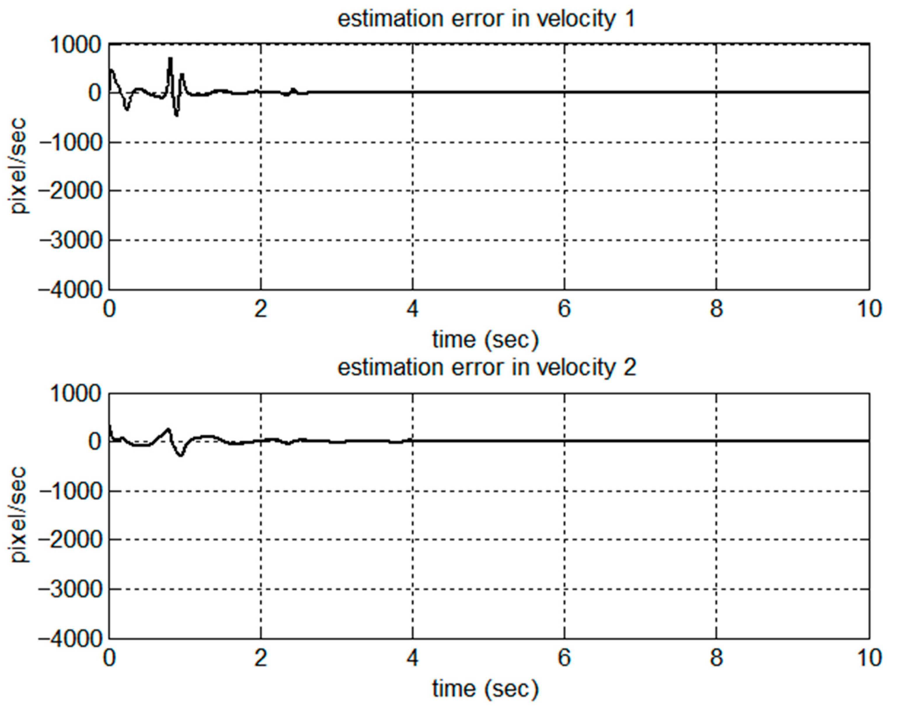
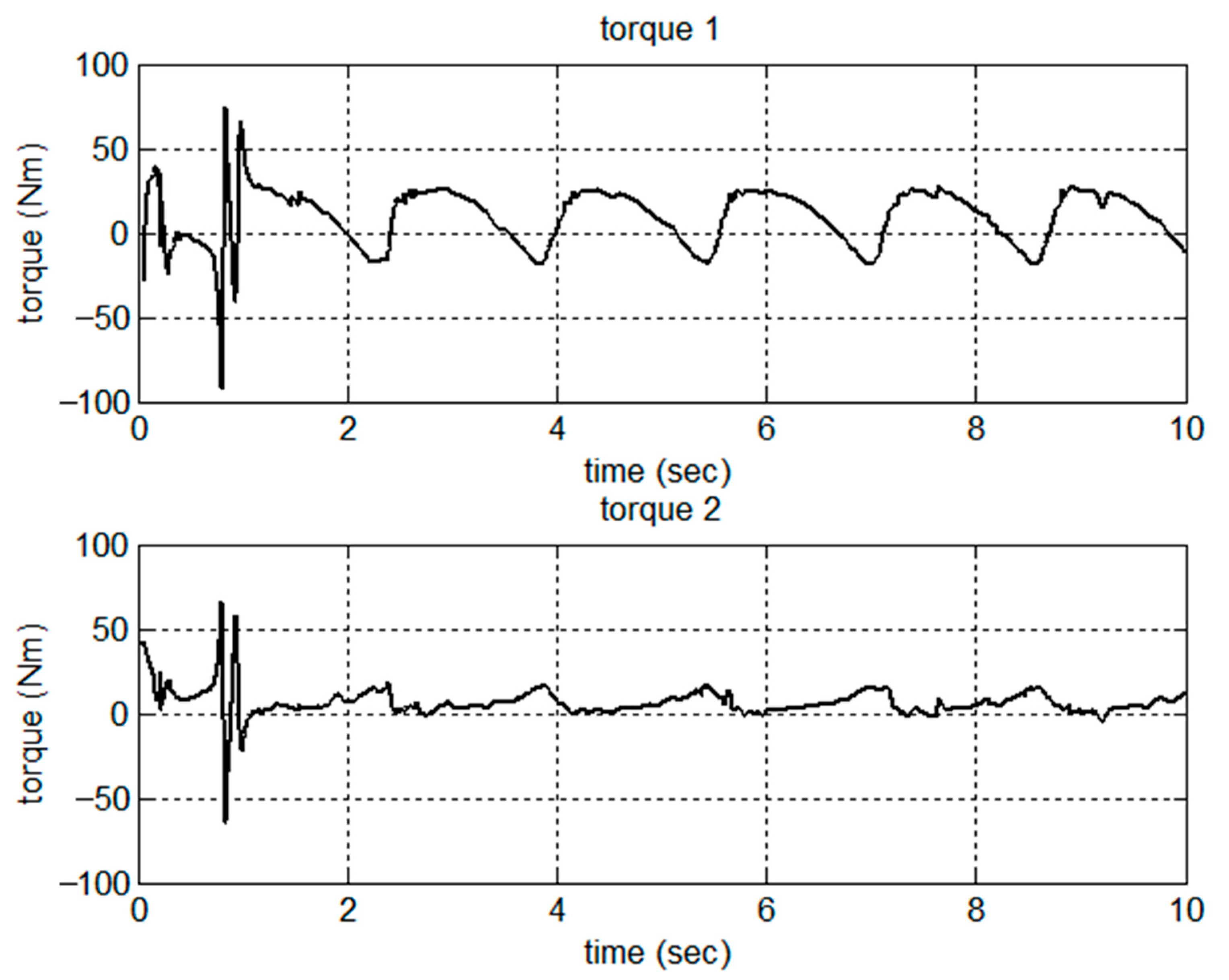
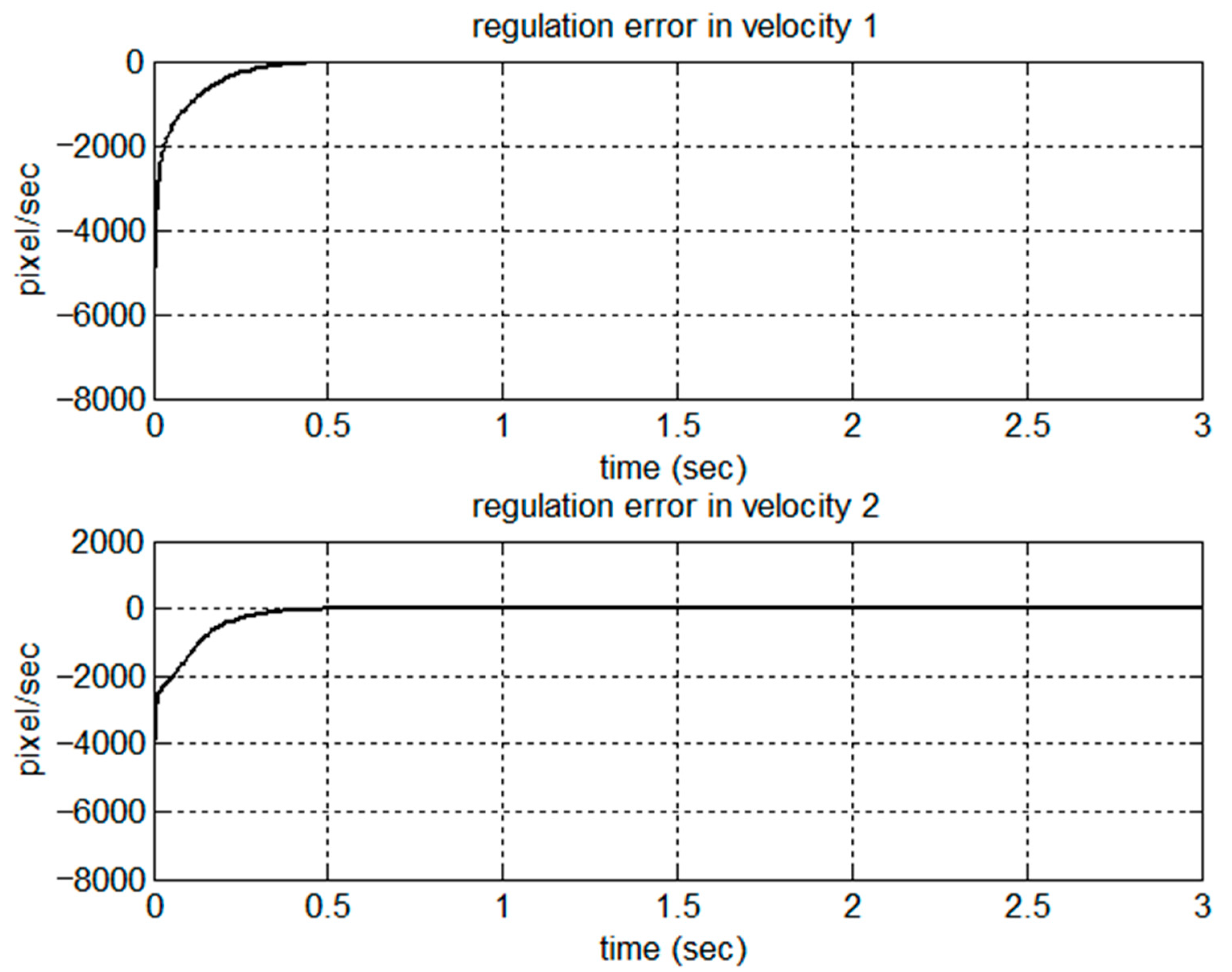
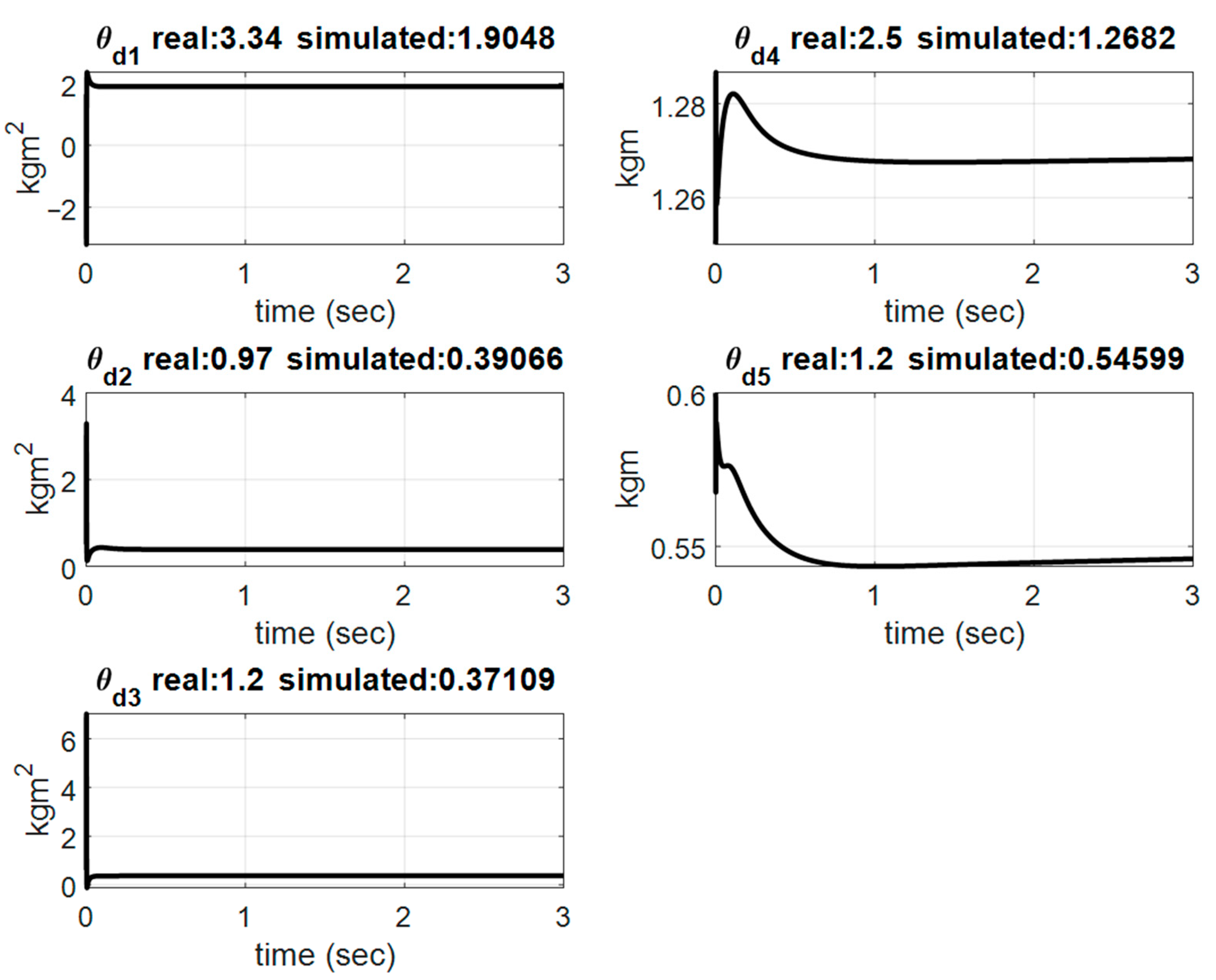
5.3. Simulation Results

Figure 2, Figure 3, Figure 4, Figure 5, Figure 6, Figure 7, Figure 8 and Figure 9 show the simulation results of the proposed scheme on the two-link robot for trajectory tracking. The position trajectories in the task space are shown in Figure 2. The tracking error in terms of position and velocity is shown in Figure 3 and Figure 4, respectively. Clearly, from the simulation results, without the velocity measurement in the task space, the proposed control scheme could successfully track the desired trajectory in the case of uncertain parametric dynamics and kinematics parameters. The convergence rate could be modified by the choice of design parameters. We can see from the parameter estimation shown in Figure 5 that the dynamic parameters were bounded and convergent. According to the stability analysis, it can be understood that there was no guarantee of convergence to the true value of dynamic parameters. In contrast to the results of dynamic parameters, the kinematic parameters shown in Figure 6 converged to the true values for trajectory tracking. The estimation tracking errors for position and velocity are shown in Figure 7 and Figure 8, respectively. The observer successfully estimated the velocity in the task space without measurement. Figure 9 presents the control torques for the trajectory tracking in the task space.

5.4. Comparison

A comparative simulation of set-point control was conducted by using the proposed adaptive control schemes for the same model and the parameters described in Section 5.1. The simulation results are shown in Figure 10, Figure 11, Figure 12, Figure 13, Figure 14, Figure 15, Figure 16 and Figure 17 for the set-point control. As shown in Figure 10, the robot was driven from the initial point [863 554] in the image frame to the desired point [540 200] in 0.5 s. The regulation errors in positions and velocities are shown in Figure 11 and Figure 12, respectively. Figure 13 presents the estimation of dynamic parameters. In particular, from the simulation results shown in Figure 14, we can see that the kinematic parameters were not necessarily converging to the true values due to the rank deficiency of the kinematic regressor. Figure 15 and Figure 16 show the estimation errors in terms of positions and velocities. Due to the set-point control, the control torques reached the steady state after 0.5 s, as shown in Figure 17.

6. Conclusions

In this paper, we present a simple solution to the problem of task-space robot tracking control under the parametric uncertainties in both kinematics and dynamics. We proposed an adaptive control scheme with adaptation laws and designed a new observer to estimate velocities in the task space. Using the Lyapunov stability and Barbalat’s lemma, we show that the tracking errors and estimation errors in task space can asymptotically converge to zero. Furthermore, we used a two-link robot with a fixed camera to verify the proposed adaptive control and the task-space velocity observer. From the simulation results on the trajectory tracking and the set-point control, the proposed control scheme can effectively accomplish the control goal in the presence of kinematic and dynamic uncertainties. Note that this paper only considers non-singular Jacobian cases. How to identify and deal with the singular Jacobian situation to make the control operate appropriately requires further research. In the future, we will conduct experimental evaluations of the proposed adaptive control and extend the control scheme to networked robot systems.

References

1. Ruiz, L.; Torres, M.; Gómez, A.; Díaz, S.; González, J.M.; Cavas, F. Detection and Classification of Aircraft Fixation Elements during Manufacturing Processes Using a Convolutional Neural Network. Appl. Sci. 2020, 10, 6856. [Google Scholar] [CrossRef]
2. Craig, J.J.; Hsu, P.; Sastry, S.S. Adaptive control of mechanical manipulators. Int. J. Robot. Res. 1987, 6, 16–28. [Google Scholar] [CrossRef]
3. Middleton, R.H.; Goodwin, G.C. Adaptive computed torque control for rigid link manipulators. Syst. Control Lett. 1988, 10, 9–16. [Google Scholar] [CrossRef]
4. Spong, M.W.; Ortega, R. On adaptive inverse dynamics control of rigid robots. IEEE Trans. Autom. Control 1990, 35, 92–95. [Google Scholar] [CrossRef]
5. Slotine, J.J.E.; Li, W. Adaptive manipulator control: A case study. IEEE Trans. Autom. Control 1988, 33, 995–1003. [Google Scholar] [CrossRef]
6. Cheah, C.C.; Hirano, M.; Kawamura, S.; Arimoto, S. Approximate Jacobian control for robots with uncertain kinematics and dynamics. IEEE Trans. Robot. Autom. 2003, 19, 692–702. [Google Scholar]
7. Cheah, C.C.; Liu, C.; Slotine, J.J.E. Adaptive tracking control for robots with unknown kinematic and dynamic properties. Int. J. Robot. Res. 2006, 25, 283–296. [Google Scholar] [CrossRef]
8. Cheah, C.C.; Liu, C.; Slotine, J.J.E. Adaptive Jacobian Tracking Control of Robots with Uncertainties in Kinematic, Dynamic and Actuator Models. IEEE Trans. Autom. Control 2006, 51, 1024–1029. [Google Scholar] [CrossRef]
9. Wang, H.; Liu, Y.H.; Zhou, D. Dynamic visual tracking for manipulators using an uncalibrated fixed camera. IEEE Trans. Robot. 2007, 23, 610–617. [Google Scholar] [CrossRef]
10. Braganza, D.; Dixon, W.E.; Dawson, D.M.; Xian, B. Tracking control for robot manipulators with kinemtic and dynamic uncertainty. Int. J. Robot. Autom. 2008, 23, 117–126. [Google Scholar]
11. Cheah, C.C. Task-space PD control of robot manipulators: Unified analysis and duality property. Int. J. Robot. Res. 2008, 27, 1152–1170. [Google Scholar] [CrossRef]
12. Wang, H.; Xie, Y. Adaptive inverse dynamics control of robots with uncertain kinematics and dynamics. Automatica 2009, 45, 2114–2119. [Google Scholar] [CrossRef]
13. Cheah, C.C.; Liu, C.; Slotine, J.J.E. Adaptive Jacobian vision based control for robots with uncertain depth information. Automatica 2010, 46, 1228–1233. [Google Scholar] [CrossRef]
14. Wang, H.; Liu, Y.; Chen, W. Uncalibrated Visual Tracking Control Without Visual Velocity. IEEE Trans. Control Syst. Technol. 2010, 18, 1359–1370. [Google Scholar] [CrossRef]
15. Liang, X.; Huang, X.; Wang, M.; Zeng, X. Adaptive Task-Space Tracking Control of Robots Without Task-Space- and Joint-Space-Velocity Measurements. IEEE Trans. Robot. 2010, 26, 733–742. [Google Scholar] [CrossRef]
16. Wang, H.; Liu, Y.; Chen, W. Visual tracking of robots in uncalibrated environments. Mechatronics 2012, 22, 390–397. [Google Scholar] [CrossRef]
17. Li, X.; Cheah, C.C. Global task-space adaptive control of robot. Automatic 2013, 49, 58–69. [Google Scholar] [CrossRef]
18. Wang, H. Passivity based synchronization for networked robotic systems with uncertain kinematics and dynamics. Automatica 2013, 49, 755–761. [Google Scholar] [CrossRef]
19. Spong, M.W.; Hutchinson, S.; Vidyasagar, M. Robot Modeling and Control; John Wiley & Sons: Hoboken, NJ, USA, 2006. [Google Scholar]
20. Krstic, M.; Kanellakopoulos, I.; Kokotovic, P. Nonlinear and Adaptive Control Design; John Wiley & Sons: New York, NY, USA, 1995. [Google Scholar]
Figure 1. Adaptive tracking control scheme.
Applsci 10 08806 g001
Figure 2. Trajectories in the task space.
Applsci 10 08806 g002
Figure 3. Tracking error in positions.
Applsci 10 08806 g003
Figure 4. Tracking error in velocities.
Applsci 10 08806 g004
Figure 5. Estimates of dynamic parameters.
Applsci 10 08806 g005
Figure 6. Estimation of kinematic parameters.
Applsci 10 08806 g006
Figure 7. Estimation in positions.
Applsci 10 08806 g007
Figure 8. Estimation error in velocities.
Applsci 10 08806 g008
Figure 9. Control torques.
Applsci 10 08806 g009
Figure 10. Trajectories in the task space.
Applsci 10 08806 g010
Figure 11. Regulation error in positions.
Applsci 10 08806 g011
Figure 12. Regulation error in velocities.
Applsci 10 08806 g012
Figure 13. Estimation of dynamic parameters.
Applsci 10 08806 g013
Figure 14. Estimation of kinematic parameters.
Applsci 10 08806 g014
Figure 15. Estimation in positions.
Applsci 10 08806 g015
Figure 16. Estimation error in velocities.
Applsci 10 08806 g016
Figure 17. Control torques.
Applsci 10 08806 g017
Publisher’s Note: MDPI stays neutral with regard to jurisdictional claims in published maps and institutional affiliations.