Abstract
Box delivery is a complicated manual material handling task which needs to consider the box weight, delivering speed, stability, and location. This paper presents a subtask-based inverse dynamic optimization formulation for determining the two-dimensional (2D) symmetric optimal box delivery motion. For the subtask-based formulation, the delivery task is divided into five subtasks: lifting, the first transition step, carrying, the second transition step, and unloading. To render a complete delivering task, each subtask is formulated as a separate optimization problem with appropriate boundary conditions. For carrying and lifting subtasks, the cost function is the sum of joint torque squared. In contrast, for transition subtasks, the cost function is the combination of joint discomfort and joint torque squared. Joint angle profiles are validated through experimental results using Pearson’s correlation coefficient (r) and root-mean-square-error (RMSE). Results show that the subtask-based approach is computationally efficient for complex box delivery motion simulation. This research outcome provides a practical guidance to prevent injury risks in joint torque space for workers who deliver heavy objects in their daily jobs.
1. Introduction
The box delivery process includes multi-task jobs (e.g., that involves box lifting, carrying, and lowering it). In multi-task case, workers combine subtasks with transition phases which affect the pace, posture, motion, and the resulting biomedical loads of the workers [1]. Biomechanical modeling provides a useful tool to investigate the cause and effect without worrying about injury risks. However, it proves that simulating a human delivering motion is a challenging task. The objective of this study is to explore the subtask-based inverse dynamic optimization formulation to efficiently analyze and predict dynamic human delivering motion in ergonomic applications.
The box delivery task can be divided into four main subtasks: lifting, carrying, transition, and unloading. The transition task includes the motion from lifting to carrying and carrying to unloading with varied boundary conditions. Each subtask can be formulated as an optimization problem by associating boundary conditions between the two adjacent subtasks.
The task decomposition approach was used to simulate walking motion with double support and single support phases [2], but only few studies have been conducted on the delivery task (multi-task jobs). Here is a summary of the literature for carrying, lifting, and transition tasks. There are two different methods for optimization-based lifting planning problems: static lifting optimization [3,4] and dynamic lifting optimization [5,6,7,8,9]. Various cost functions were used in the optimization formulation, such as muscle intensity [3], joint torque squared [7], compressive force on spine [10], and smoothness of the lifting motion [6,8]. Noone and Mazumdar [3] investigated various cost functions for static lifting using a simple geometrical model. They found that muscle intensity was a more efficient cost function for lifting. Three objective functions for optimal lifting postures were studied by Dysart and Woldstad [4]. They concluded that minimizing the overall effort generated the most accurate motion with subject validation. In addition, the hand’s relative height location was an important factor for the accuracy of the prediction. Kromodihardjo and Mital [10] calculated the stresses on major joints using a 2D biomechanical lifting model. The effects of lifting technique on the spine was investigated.
Hsiang and McGorry [6] studied three cost functions using dynamic lifting simulation. The three cost functions were: to minimize the sudden kinematic variance of the center of gravity, to maximize the lifting motion’s smoothness, and to minimize the sum of joint torque squared. They found that the peak spine loads were minimal when the load took the smoothest path. Gazula et al. [11] simulated a tossing motion with three phases. It was found that mobilization and torque utilization were important cost functions in the final phase of tossing. Xiang et al. [7] aggregated dynamic effort and stability objective functions to predict lifting motion using a multi-objective optimization method. The proposed approach successfully found the optimal lifting motion which was validated with experimental data.
The lifting height and weight correlate with the shear and compressive forces on the spine. Many task-analysis tools (e.g., the revised NIOSH lifting equation) are rooted in a task-based analysis approach [12]. These tools divide the multi-task jobs into single subtasks and analyze each individual subtask separately, and synthesize the results into the entire job. Several studies reported differences in the metabolic rates, perceived exertion, heart rates, hand forces, compression, and shear forces of workers when they performed these multi-task jobs compared to single-task jobs [13,14,15,16]. It has been concluded that the risk of injury during multi-task jobs could not be accurately assessed using tools that analyze single tasks [13,14,17]. Therefore, it is necessary to develop a subtask-based simulation formulation to analyze the kinematic and dynamic for multi-task jobs, and this is the first step towards the ultimate goal to prevent injuries for various tasks through biomechanical modeling.
Currently, there is plenty of research for optimizing and simulating walking. The carrying motion is rooted in walking [18,19,20,21]. Carrying can be simulated by applying loads on hands using the gait simulation method [22]. Two transitions, slow to fast walking and walking to standing, were studied by Xiang et al. [23] using a predictive model.
In this study, the subtask-based inverse dynamic optimization is used for 2D box delivery simulation. This method has some advantages over the traditional forward dynamic simulation in terms of computational efficiency [24,25,26,27]; this is because equations of motion are directly evaluated from inverse dynamics in each optimization iteration.
Although each subtask of the delivery task has been solved in many ways in the literature [21,22,23], a complete delivery motion prediction can be difficult. The objective of this study is to investigate a subtask-based formulation that can generate a delivery motion from the start to the end. In addition, it is desirable to make the optimization problem with less computing effort, easy to implement and more accurate.
The rest of this paper is organized as follows. The skeletal human model is first described in Section 2. Section 3 presents motion capture experimental data collection. Section 4 presents subtask-based optimization formulation, and box delivery simulation results are presented in Section 5. Finally, the discussion and conclusion are given in Section 6.
2. 2D Skeletal Human Model
Figure 1 shows a 2D skeletal model which has 14 degrees of freedom (DOFs). This skeletal model is adopted to simulate symmetric delivery motion. Three DOFs are used for global rotation (β) and translation (y, z), and 11 DOFs () are used for modeling the human body joints. The global DOFs consist of one revolute joint and two prismatic joints. The left and right legs and arms are assumed to be symmetric. There are three body branches: two leg branches and one spine-arm branch. Each leg has a thigh, a shin, a hinder foot, and a forefoot. In the arm branch, two arms are combined as a single arm branch, because only 2D motion in sagittal plane is studied. The 50th percentile anthropometric data from the experimental subjects are used for the skeletal model.
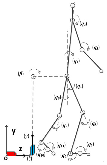
Figure 1.
The 2D skeletal model.
Figure 1 shows how the DOFs are built in the Denavit–Hartenberg (DH) approach [28]. The DOF of each joint is defined in the local z-direction. In global Y-Z plane, the positive directions for the body rotation joints () are clockwise. The global rotation joint (β), spine joint (), and two hip joints ( and ) coincide at the same location. A recursive Lagrangian dynamics formulation is utilized for this model, and the ground reaction force (GRF) is calculated from the gravity, joint kinematics, and external loads by a two-step inverse procedure [21]. The details are presented by Xiang et al. [29]. The forward joint kinematics are calculated as:
where is the ith joint angle; is the link transformation matrix from the (i − 1)th link frame to the ith link frame; , , and are global position, velocity, and acceleration transformation matrices, respectively; and , .
The backward joint torque equations are defined as follows:
where is the trace of a matrix, is the inertia matrix for link i, is the matrix for inertia and Coriolis, is the external force torque vector, is the gravity torque vector, is the external moment torque vector, is the gravity vector, is the center of mass of link i, is the mass of link i, is the external moment applied on link k, is the external force applied on link k, is the position of the external force in the local frame k, is for a prismatic joint, is for a revolute joint, is Kronecker delta, and the starting conditions are , .
3. Motion Capture Experiments
Motion capture experimental data collection was performed, and the experimental protocol was approved by the internal review board (IRB) at Texas Tech University. In total, 20 subjects were recruited for the study. Among them, two were discarded because of incomplete capture data.
3.1. Participants
The subjects were chosen for the 50th percentile stature and body mass. Participants were all male (age: 23.07 ± 1.64 years; height: 175.46 ± 4.93 cm; body mass: 71.77 ± 5.42 kg, where ± means standard deviation). All subjects were physically and mentally sound and signed an informed consent form.
3.2. Data Collection
An optical sensor-based motion capture system was used. The system included 7 Eagle-4 camera systems (Motion Analysis Corporation, Rohnert Park, CA, USA). Each camera has a four-megapixel resolution with maximum 500 fps (frames per second). A 3.04 × 3.04 m2 area was selected for the delivery task with cameras surrounding at a height of around 2.74 m. Fifty-two retroreflective markers were placed on the bodies of the subjects. The markers were placed such that the markers move as little as possible on the body followed the protocol developed by Cloutier et al. [30]. Stature and body mass were recorded for each participant before experiment. Experimental setup is shown in Figure 2.
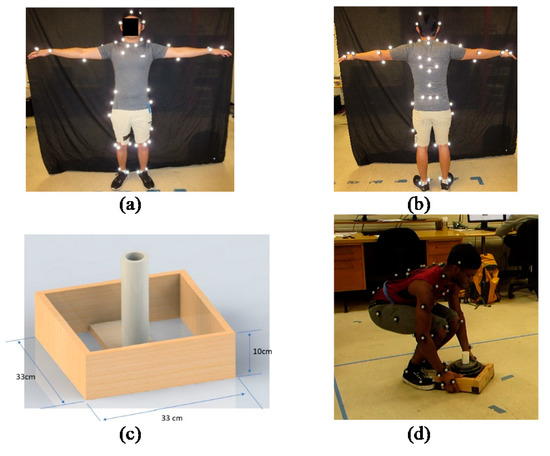
Figure 2.
Experimental setup: (a) marker placement protocol front view; (b) marker placement protocol back view; (c) box dimension and weight, without external load: 2.36 Kg, with external load: 10.16 Kg; and (d) experiment environment, where the average distance between initial and final position is 2.4 m and the table height of the final position from ground is 0.5 m.
Before the experiment test started, participants were asked to walk five steps ahead from the initial position. Depending on the step length, the table was set to be in an appropriate distance to the subject’s final step. Each participant was requested to finish the following tasks in the following order: (1) stand in parallel feet behind box; (2) pick the box up to a comfortable waist height; (3) walk five steps starting from the left leg including initial transition step, three intermediate carrying steps, and final transition step; (4) stand in front of a 0.5 m height table; and (5) unload the box on the table. The same procedure was repeated 3 times for each subject.
3.3. Data Processing
GEBOD, a regression-based interactive utility [31], was used to generate each subject’s body segment centers of mass, lengths, and inertial properties. The inputs for GEBOD include the subject’s gender, age, stature height, and body weight.
All markers were labeled in Cortex (Motion Analysis Corporation, Rohnert Park, CA, USA). Spine, right elbow, right shoulder, right knee, and right hip joint angles were calculated from motion capture data for each subject. Average and standard deviation were then calculated for all 18 subjects.
4. Subtask-Based Optimization Formulation
A complete delivery task has five subtasks: (1) an initial lifting, (2) the transition step from the final lifting posture to a start of the carrying gait, (3) a carrying motion, (4) the transition step from the final carrying posture to a standing posture, and (5) the final delivering by placing the box on a table. The final and initial lifting postures, final and initial unloading postures, footstep lengths, and time durations are all given from experiments. Figure 3 shows the detailed procedure and relationship among different subtask optimization formulations.
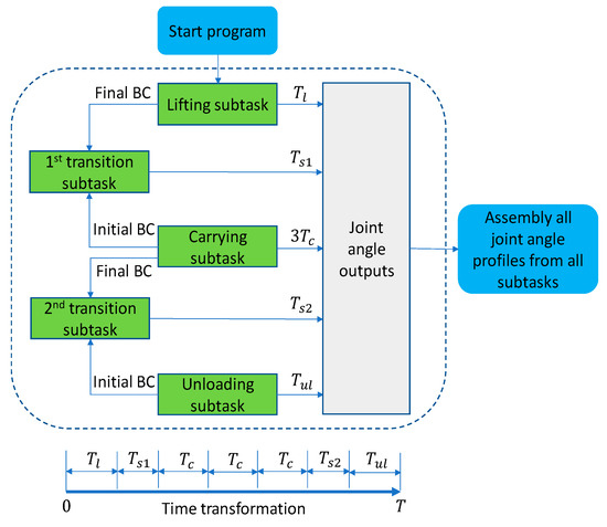
Figure 3.
Flow chart of the subtask-based formulation (where BC denotes boundary conditions including joint angle and angular velocity, is lifting time duration, is 1st transition time duration, is carrying time duration, is 2nd transition time duration,
is unloading time duration, is total box delivery time duration).
4.1. Lifting and Unloading Subtasks
For the lifting subtask, the total lifting time, initial and final postures, and lifting weight are specified in the simulation from the experimental mean values. The design variables are joint angle profile cubic B-spline control points (). The cost function is the sum of the normalized joint torque squared as in Equation (9) for the lifting period .
where is the number of DOF, is the upper limit for the ith joint torque, and is the lower limit for the ith joint torque.
The lifting subtask is subject to the following constraints:
Joint angle limits,
where is the lower joint angle limit and is the upper joint angle limit.
Joint torque limits,
In addition, the feet contacting positions are given from experiments,
where is the calculated foot position, and is the measured Cartesian coordinates of footstep position during delivering motion based on the mean experimental step lengths.
The foot is contacting the ground, the height of the foot-contacting points is zero. The other points’ heights should be greater than zero.
where i is the point index on foot which is contacting the ground [21].
Balance is considered during the box delivering process using the zero-moment point (ZMP) constraint,
where FSR is the foot support region, and is the ZMP location. This constraint is defined by constraining the sign of cross product of two vectors: one vector is composed of ZMP and FSR vertex, the other vector is the adjacent FSR boundary. This process is repeated until all FSR boundaries are satisfied. Details are given in reference [32].
Collision avoidance between box and body,
where is the radius of the circle filled in the body segment, is half of the box width, and d is the distance between each circle center and the hand. There are five circles filled in the lower body at hip, knee, ankle, mid of shank, and mid of tibia, respectively. In addition, there are two circles filled on spine to represent low spine and high spine segments.
The differences of joint angle between the experiment and the skeletal model are constrained in a small range degrees at initial and final lifting/unloading postures, where is the experimental joint angle.
It is noted that the unloading subtask starts with holding the box at a higher position and ending at a lower position during the time period . The optimization formulation for unloading subtask is similar to the lifting subtask.
4.2. Carrying Subtask
In this study, only one step carrying motion was simulated. The second step carrying motion was obtained by using the lower body symmetric and upper body continuity conditions. For the carrying subtask, given values consisted of experimental means of step length, walking speed, box relative position to pelvis, and the box weight.
The design variables are joint angle profile cubic B-spline control points (). The cost function is the sum of the normalized joint torque squared as in Equation (9) by replacing the joint angle control points with for one step carrying motion period . The constraints for the one step carrying are defined in Equations (10)–(15). Additional constraints for one step carrying motion includes knee flexion at mid-swing, upper body joint angles, upper body continuity conditions, and lower body symmetric conditions as in Equations (17)–(19).
Knee flexion at mid-swing is around sixty degrees to avoid foot drag motion,
where is the experimental mean value determined at 75% of the gait cycle [21].
The upper body joint angles are constrained to the experimental mean values during one step carrying motion,
where is the experimental mean and degrees.
Finally, the lower body satisfies symmetric constraints, and upper body satisfies continuity constraints at time boundaries.
where is the right and left symmetric joint angles for lower body, .
4.3. Transition Subtask
For the lifting to carrying transition subtask, the transitioning was from standing with two feet contacting the ground to carrying gait cycle with a double foot support phase. For the subtask of transition, given values consisted of transition time duration, step length, final and initial boundary joint angles and velocities from lifting, unloading, and carrying subtask simulations.
The design variables are joint angle profile cubic B-spline control points (). The objective function is to minimize the joint torque squared and the joint angle discomfort [33], as follows:
where is the time duration of transition subtask, is the average of the ith final and initial boundary joint angle values, is the coefficient for the discomfort function, is the coefficient for the torque squared cost function. and are chosen so that the values of the two cost functions have same magnitude. The constraints for the transition subtask are defined in Equations (10)–(15) and Equation (17) as in Table 1. An additional constraint for transition subtask is boundary conditions from other subtasks, where and are boundary joint angles and angular velocities.

Table 1.
Constraints for subtasks.
4.4. Assembling Results of All Subtasks to a Complete Delivery Task
For object delivery motion simulation, the simulated lifting, carrying, and unloading motions were stitched together by transition subtasks to render one complete delivery task.
For the optimization of the components, the lifting and carrying subtasks were first simulated; the final postures and velocities of the lifting and the initial postures and velocities of the carrying were imported into the first transition subtask to make a smooth motion. Then, carrying motion had 3 steps before entering the second transition subtask. Next, the unloading subtask was simulated, and the initial/final (depending on even or odd steps) postures and velocities of the carrying and the initial postures and velocities of the unloading were imported into the second transition subtask to generate a seamless delivery motion. Finally, all subtask output data were stitched together in a correct order in the algorithm written in MATLAB® to generate a whole delivery motion. A batch script was written for automatically running each subtask optimization, exporting boundary files, and rendering the complete delivery motion [34].
5. Simulation Results and Validation
The SNOPT [35] was used to solve the optimization problem with the sequential quadratic programming algorithm. SNOPT has four solvers; the solver NPOPT was used in this study to solve the dense nonlinear optimization problem [35]. By following the flowchart in Figure 3, the simulation results were obtained by solving the subtask-based optimization problem based on the input data from experiments (mean values from all subjects). Figure 4 shows the resulting optimal delivery motion snapshots. Figure 5 shows the comparison of the joint angle profiles from the subtask-based optimization formulation with the experimental results. The joint torque profiles are shown in Figure 6. Table 2 lists the total number of design variables, constraints, and Central Processing Unit (CPU) times for the subtask-based approach. A laptop computer with an Intel(R) Core(TM) i5-1035G4 CPU@1.10 GHz and 8 GB RAM was used to solve the optimization problem. Table 3 lists the root-mean-square-error (RMSE) and Pearson’s correlation coefficient (r) for comparing the predicted and experimental joint angle profiles.
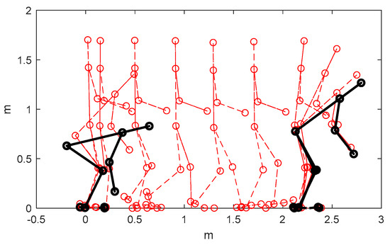
Figure 4.
Predicted optimal delivery motion snapshots for a 10.16 Kg box.
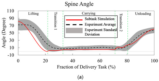
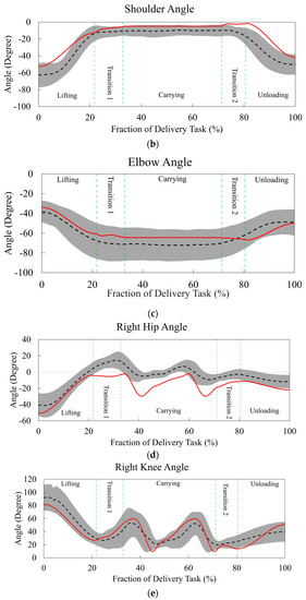
Figure 5.
Joint angle profiles for deliver motion: (a) spine, (b) shoulder, (c) elbow, (d) right hip, and (e) right knee.
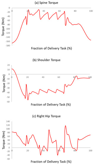
Figure 6.
Joint torque profiles for deliver motion: (a) spine, (b) shoulder, and (c) right hip.

Table 2.
Optimization information for subtask-based approach.

Table 3.
Root-mean-square-error (RMSE) and Pearson correlation coefficient (r) averaged across 18 subjects; values are represented as mean (standard deviation).
6. Discussion and Conclusions
In this study, the subtask-based optimization approach has been presented to predict the box delivery motion. A motion capture experiment was conducted to collect kinematic data for box delivery validation. In addition, results from the simulation were compared with the experimental data.
In Figure 5, the predicted joint angles (spine, shoulder, elbow, right knee) for the subtask method lie within the standard deviation of the mean for the major portion of the motion and also follow the similar trend as the experimental mean, indicating reasonable agreement with the experimental results. For the right hip angle in Figure 5d, the carrying motion has a similar trend as the experimental mean but is outside the standard deviation. The minimum values are outside of the experimental standard deviation. This is because we did not impose experimental boundary conditions for carrying simulation, instead the carrying motion only satisfies symmetry and continuity boundary conditions on itself. Two transition subtasks took place at around 20–30% and 70–80% time periods, respectively. Joint discomfort objective function was used to reduce the redundant motion for the subtask-based approach as seen in Figure 5. For lifting and unloading motions, although the experimental boundary constraints were imposed, the spine and shoulder joint angles are still partially outside the standard deviation between the boundaries as seen in Figure 5a,b.
For transition motion in Figure 5, the continuity boundary conditions were imposed on joint angles and angular velocities only, not on joint accelerations as shown in Equation (21). Therefore, there were small jerks at transitions. However, if we also imposed the joint acceleration continuity constraint, it would make the optimization design space too tight, and the optimization problem difficult to converge. In addition, the hip joint angle profile deviated from the experimental data during the carrying motion. This is because we did not use any experimental data for the lower body during carrying motion. The amount of experimental data used in the optimization formulation compromises the power of prediction. Here, we find a balance between them. The proposed optimization formulation for carrying motion predicts knee and ankle joint angles well without relying on lower body experimental data.
The spine, shoulder, and right hip joint torque profiles in Figure 6 showed repeatable patterns during carrying motion as expected. For the subtask-based approach, there were oscillations of torque values at the boundaries of transition phase. This is due to the discontinuity of joint acceleration between subtasks in the model.
The total CPU time for the subtask-based method was 6.71 s, as seen in Table 2. It is shown that each subtask is a small-scale optimization problem so that the subtask-based method converges fast. If we simulated a box delivery motion with more carrying steps as one single task optimization problem, the convergence time could be longer. In contrast, the CPU time for the subtask-based approach did not change with the increasing number of carrying steps because the carrying gait can repeat on itself.
It can be seen from Table 3 of the RMSE and Pearson’s coefficient that the formulation could provide reasonable results. The major advantages of the proposed subtask-based optimization method include: First, each subtask is a relatively small scale optimization problem which is easy to formulate based on the well-studied subtask in the literature [7,22,23]. Secondly, the subtask simulation is computationally efficient and is close to real-time implementation. Third, each subtask can be formulated as a separate optimization problem with different cost functions. For example, in this study, we introduced a discomfort function for the transition subtask to make the transitional motion smoother, as seen in Figure 5.
The contributions of this study are as follows: (1) this work is the first study of predictive object delivery formulation using a subtask-based approach in the literature, and it is the first step to investigate the complete delivery motion formulation, which establishes a solid foundation to understand the delivery task; (2) the proposed predictive delivery formulation depends on little experimental data, which is important to guide the prediction [36]. Previous work comprises mainly empirical studies based on experimental data—i.e., data-driven approach [37]; (3) feasibility of the subtask-based approach for predictive delivery task simulation; (4) the subtask-based approach is computationally efficient, which is critical for future musculoskeletal delivery simulation.
In future, we will validate GRF, Electromyography (EMG), and simulate more complicated three-dimensional motion using the proposed subtask-based optimization method.
Author Contributions
Y.X.; methodology, Y.X. and P.O.; software, P.O.; validation, S.T. and J.Y.; formal analysis, Y.X., P.O., and S.T.; investigation, Y.X.; resources, Y.X. and J.Y.; data curation, Y.X., P.O., and S.T.; writing—original draft preparation, Y.X.; writing—review and editing, Y.X. and J.Y.; visualization, Y.X. and S.T.; supervision, Y.X. and J.Y.; project administration, Y.X. and J.Y.; funding acquisition, Y.X. and J.Y. All authors have read and agreed to the published version of the manuscript.
Funding
This research was funded by National Science Foundation, grant number 1849279 and 1703093 and The APC was funded by NSF grant 1849279.
Acknowledgments
We thank Adrian Harvey, undergraduate researcher from Texas Tech University for helping in experimental data collection.
Conflicts of Interest
The authors declare no conflict of interest.
References
- Harari, Y.; Bechar, A.; Riemer, R. An investigation of workplace design and the worker’s anthropometrics influence on work pace during manual material handling tasks. In Proceedings of the 2016 Human Factors and Ergonomics Society Annual Meeting, Washington, DC, USA, 19–23 September 2016; pp. 727–728. [Google Scholar]
- Saidouni, T.; Bessonnet, G. Generating globally optimised sagittal gait cycles of a biped robot. Robotica 2003, 21, 199–210. [Google Scholar] [CrossRef]
- Noone, G.; Mazumdar, J. Lifting low-lying loads in the sagittal plane. Ergonomics 1992, 35, 65–92. [Google Scholar] [CrossRef]
- Dysart, M.J.; Woldstad, J.C. Posture prediction for static sagittal-plane lifting. J. Biomech. 1996, 29, 1393–1397. [Google Scholar] [CrossRef]
- Hsiang, S.M.; Ayoub, M.M. Development of methodology in biomechanical simulation of manual lifting. Int. J. Ind. Ergon. 1994, 13, 271–288. [Google Scholar] [CrossRef]
- Hsiang, S.M.; McGorry, R.W. Three different lifting strategies for controlling the motion patterns of the external load. Ergonomics 1997, 40, 928–939. [Google Scholar] [CrossRef]
- Xiang, Y.; Arora, J.S.; Rahmatalla, S.; Marler, T.; Bhatt, R.; Abdel-Malek, K. Human lifting simulation using a multi-objective optimization approach. Multibody Syst. Dyn. 2010, 23, 431–451. [Google Scholar] [CrossRef]
- Song, J.; Qu, X.; Chen, C.H. Simulation of lifting motions using a novel multi-objective optimization approach. Int. J. Ind. Ergon. 2016, 53, 37–47. [Google Scholar] [CrossRef]
- Xiang, Y.; Zaman, R.; Rakshit, R.; Yang, J. Subject-specific strength percentile determination for two-dimensional symmetric lifting considering dynamic joint strength. Multibody Syst. Dyn. 2019, 46, 63–76. [Google Scholar] [CrossRef]
- Kromodihardjo, S.; Mital, A. Biomechanical analysis of manual lifting tasks. J. Biomech. Eng. 1987, 109, 132–138. [Google Scholar] [CrossRef] [PubMed]
- Gazula, H.; Chang, C.C.; Lu, M.L.; Hsiang, S.M. Using mutual information to capture major concerns of postural control in a tossing activity. J. Biomech. 2015, 48, 1105–1111. [Google Scholar] [CrossRef]
- Dempsey, P.G.; Mathiassen, S.E. On the evolution of task-based analysis of manual materials handling, and its applicability in contemporary ergonomics. Appl. Ergon. 2006, 37, 33–43. [Google Scholar] [CrossRef] [PubMed]
- Straker, L.M.; Stevenson, M.G.; Twomey, L.T. A comparison of risk assessment of single and combination manual handling tasks: 2. Discomfort, rating of perceived exertion and heart rate measures. Ergonomics 1997, 40, 656–669. [Google Scholar] [CrossRef] [PubMed]
- Straker, L.M.; Stevenson, M.; Twomey, L.T.; Smith, L.M. A comparison of risk assessment of single and combination manual handling tasks: 3. Biomechanical measures. Ergonomics 1997, 40, 708–728. [Google Scholar] [CrossRef]
- Dempsey, P.G.; Ciriello, V.M.; Maikala, R.V.; O’Brien, N.V. Oxygen consumption prediction models for individual and combination materials handling tasks. Ergonomics 2008, 51, 1776–1789. [Google Scholar] [CrossRef]
- Taboun, S.; Dutta, S. Energy cost models for combined lifting and carrying tasks. Int. J. Ind. Ergon. 1989, 4, 1–17. [Google Scholar] [CrossRef]
- Straker, L.M.; Stevenson, M.G.; Twomey, L.T. A comparison of risk assessment of single and combination manual handling tasks: 1. Maximum acceptable weight measures. Ergonomics 1996, 39, 128–140. [Google Scholar] [CrossRef]
- Bessonnet, G.; Marot, J.; Seguin, P.; Sardain, P. Parametric-based dynamic synthesis of 3D-gait. Robotica 2010, 28, 563–581. [Google Scholar] [CrossRef]
- Sarka, A.; Dutta, A. Optimal trajectory generation and design of an 8-dof compliant biped robot for walk on inclined ground. J. Intell. Robot. Syst. 2019, 94, 583–602. [Google Scholar] [CrossRef]
- Shourijeh, M.S.; McPhee, J. Forward dynamic optimization of human gait simulations: A global parameterization approach. J. Comput. Nonlinear. Dyn. 2014, 9, 031018. [Google Scholar] [CrossRef]
- Xiang, Y.; Arora, J.S.; Abdel-Malek, K. Optimization-based prediction of asymmetric human gait. J. Biomech. 2011, 44, 683–693. [Google Scholar] [CrossRef]
- Xiang, Y. Human carrying simulation with symmetric and asymmetric loads using optimization. J. Appl. Biomech. 2014, 30, 140–146. [Google Scholar] [CrossRef]
- Xiang, Y.; Arora, J.S.; Chung, H.J.; Kwon, H.J.; Rahmatalla, S.; Bhatt, R.; Abdel-Malek, K. Predictive simulation of human walking transitions using an optimization formulation. Struct. Multidiscip. Optim. 2011, 45, 759–772. [Google Scholar] [CrossRef]
- Huang, C.; Sheth, P.N.; Granata, K.P. Multibody dynamics integrated with muscle models and space-time constraints for optimization of lifting movements. In Proceedings of the 2005 ASME International Design Engineering Technical Conference s and Computers and Information in Engineering Conference, Long Beach, CA, USA, 24–28 September 2005; pp. 391–398. [Google Scholar]
- Davy, D.T.; Audu, M.L. A dynamic optimization technique for predicting muscle forces in the swing phase of gait. J. Biomech. 1987, 20, 187–201. [Google Scholar] [CrossRef]
- Bessonnet, G.; Seguin, P.; Sardain, P. A parametric optimization approach to walking pattern synthesis. Int. J. Rob. Res. 2005, 24, 523–536. [Google Scholar] [CrossRef]
- Ren, L.; Jones, R.K.; Howard, D. Predictive modeling of human walking over a complete gait cycle. J. Biomech. 2007, 40, 1567–1574. [Google Scholar] [CrossRef] [PubMed]
- Denavit, J.; Hartenberg, R.S. A kinematic notation for lower pair mechanisms based on matrices. J. Appl. Mech. 1955, 22, 215–221. [Google Scholar]
- Xiang, Y.; Arora, J.S.; Abdel-Malek, K. Optimization-based motion prediction of mechanical systems: Sensitivity analysis. Struct. Multidiscip. Optim. 2009, 37, 595–608. [Google Scholar] [CrossRef]
- Cloutier, A.; Boothby, R.; Yang, J. Motion capture experiments for validating optimization-based human models. In Proceedings of the HCI-3rd ICDHM, Orlando, FL, USA, 9–14 July 2011; pp. 59–68. [Google Scholar]
- Cheng, H.; Obergefell, L.; Rizer, A. Generator of Body (GEBOD) Manual; Tech. Rep. AL.CF-TR-1994-0051; Armstrong Laboratory, Wright-Patterson Air Force Base: Dayton, OH, USA, 1994. [Google Scholar]
- Xiang, Y.; Arora, J.S.; Rahmatalla, S.; Abdel-Malek, K. Optimization-based dynamic human walking prediction: One step formulation. Int. J. Numer. Methods Eng. 2009, 79, 667–695. [Google Scholar] [CrossRef]
- Yang, J.; Marler, R.T.; Kim, H.J.; Arora, J.S.; Abdel-Malek, K. Multi-objective optimization for upper body posture prediction. In Proceedings of the 10th AIAA/ISSMO Multidisciplinary Analysis and Optimzation Conference, Albany, NY, USA, 30 August–1 September 2004; p. 4506. [Google Scholar]
- Owens, P.D. Dynamics Simulation of Human Box Delivering Task; University of Alaska Fairbanks: Fairbanks, AK, USA, 2018. [Google Scholar]
- Gill, P.E.; Murray, W.; Saunders, M.A. SNOPT: An SQP algorithm for large-scale constrained optimization. SIAM J. Optim. 2002, 12, 979–1006. [Google Scholar] [CrossRef]
- Xiang, Y.; Chung, H.J.; Kim, J.H.; Bhatt, R.; Rahmatalla, S.; Yang, J.; Marler, T.; Arora, J.S.; Abdel-Malek, K. Predictive dynamics: An optimization-based novel approach for human motion simulation. Struct. Multidiscip. Optim. 2010, 41, 465–479. [Google Scholar] [CrossRef]
- Wagner, D.W.; Kirschweng, R.L.; Reed, M.P. Foot motions in manual material handling transfer tasks: A taxonomy and data from an automotive assembly plant. Ergonomics 2009, 52, 362–383. [Google Scholar] [CrossRef] [PubMed]
Publisher’s Note: MDPI stays neutral with regard to jurisdictional claims in published maps and institutional affiliations. |
© 2020 by the authors. Licensee MDPI, Basel, Switzerland. This article is an open access article distributed under the terms and conditions of the Creative Commons Attribution (CC BY) license (http://creativecommons.org/licenses/by/4.0/).