Availability Estimation of Air Compression and Nitrogen Generation Systems in LNG-FPSO Depending on Design Stages

Abstract

This study estimated availability of an air compression system and a nitrogen generation system in liquefied natural gas—floating production storage and offloading unit (LNG-FPSO) with different design stages to investigate the gap between the availability at the early design stage and that at the late design stage. Although availability estimation in the early design stage is more important than the late design stage, it is difficult to estimate the availability accurately in the early design stage. The design stage was divided into three depending on the design progress. Monte Carlo simulation technique was employed for the availability estimation. The results of the availability estimation showed that there was 0.434% difference between the early and late design stages. This meant that the availability in the early design stage was underestimated due to limited information. A sensitivity analysis was performed to investigate critical factors affecting the results. The investigated factors were failure rate, repair time, redundant equipment, and modified preventive maintenance schedule. The most critical factor was redundant equipment. It increased 0.486% availability.

1. Introduction

Various factors are considered in system design, such as efficiency, costs, safety, and environmental effect. Availability is also one of the important issues in the system design. The definition of the availability from BS4778-3.1 (British standards, quality vocabulary, availability, reliability, and maintainability terms.) Guide to concepts and related definitions is the ability of an item under the combined aspects of reliability, maintainability, and maintenance support to perform its required function at a specified instant or for a specified period [1]. The availability indicates that how much a system approaches ideal operation without production loss caused by equipment failures or undesired external events. Availability estimation is frequently performed in the oil and gas, chemical, and power plant industries to find the optimum design option, to predict the production level, and to evaluate maintenance and operating policies.

Many previous studies conducted the availability estimation for various systems to improve their designs. Basker and Martin [2] estimated the availability of production and electrical systems using the developed numerical method. They considered failure and repair rates following the non-exponential distribution. Keller and Stipho [3] conducted the availability estimation for two similar chlorine production plants which were located in different environmental conditions (Iraq and Switzerland). They employed the concept of “delayed time” to take into account the additional time required to reach full production rate. Bosman [4] estimated the availability of a natural gas compressor plant to investigate its unavailability. Since the plant had no backup systems, the unavailability estimation was crucial. They concluded that the availability analysis provided useful information to determine the optimum number of spares. Aven [5] indicated the methodologies for the availability estimation of oil/gas production and transport systems. He described not only an analytical approach but also a simulation method for the availability estimation. Khan and Kabir [6] conducted the availability estimation for an ammonia plant using both analytical and simulation method. They concluded that the performance of the plant could be improved by changing the overhaul strategy and plant configuration. Hajeeh and Chaudhuri [7] analyzed the availability of a reverse osmosis (RO) plant for producing potable water from seawater through desalination. They employed failure mode effect analysis (FMEA) and fault tree analysis (FTA) techniques to investigate the downtime pattern and failure. Zio et al. [8] assessed the availability of an offshore installation using Monte Carlo simulation. Marquez et al. [9] suggested a general approach for the reliability and availability assessment of complex systems by employing Monte Carlo simulation. They validated the proposed approach by performing a case study for cogeneration plants. Michelassi and Monaci [10] estimated the availability of a gas re-injection plant for the oil and gas production. They utilized reliability block diagram (RBD) techniques in conjunction with Monte Carlo simulation. They also considered the leak because the plant should be stopped when the leak was detected. Chang et al. [11] estimated the availability of conventional and novel propulsion systems with a BOG handling system of an LNG carrier. They estimated the availability depending on the required function to prevent rough evaluation: design propulsion load, emergency propulsion load, and BOG utilization. Görkemli and Ulusoy [12] suggested a new modeling approach for predicting the availability of a production system. They considered not only machine failures but also the material supply, management, and set-up in the proposed method. They also investigated the uncertainties caused by the various production environment using a fuzzy Bayesian method. Seo et al. [13] predicted the availability of CO2 liquefaction processes for a ship-based carbon capture and storage (CCS) chain and they converted the availability to unavailability cost to calculate the life-cycle cost (LCC). Seo et al. [14] estimated the availability of LNG fuel gas supply systems to evaluate economics of them. They concluded that one of the significant factors was mechanical devices. Gowid et al. [15] reviewed the studies related with the profitability, reliability, and condition based monitoring of liquefied natural gas-floating production storage and offloading unit (LNG-PFSO). They assumed that the efficiency of LNG-PFOS depends on LNG liquefaction process type, system reliability, and maintenance approach, and reviewed the paper at theses points. They concluded that the literature was not sufficient to improve efficiency of LNG-FPSO. Hwang et al. [16] developed the condition-based maintenance system to perform proactive maintenance in advance to avoid the abnormal states. They addressed the system architecture, main components, diagnostics, and prognostic methods of the system.

The methodologies for the availability estimation has been improved to increase its accuracy and to apply to various systems. Precise availability estimation is important because it directly influences the owner’s decision. The availability estimation is performed several times depending on the design stages (conceptual design, basic design, and detailed design stages). In the early design stage, the results of availability estimation are effective for design improvement, but it is hard to estimate it precisely due to the limited data. On the contrary, accurate availability estimation is possible at the end of the design stage using sufficient data, but it accompanies high costs for the system modification. Therefore, it is an important to estimate the availability in the early design stage accurately. Although many studies improved the methods to increase their accuracy, there was little effort to practically estimate the availability in the early design stage

The purpose of this study is to investigate the availability gap between in the early and late design stages by estimating it with the design stages to find practical manner of availability estimation in the early design stage. The structure of this study is as follows. The target systems are described. In Section 3, methodologies for the availability estimation are discussed. The results of the availability estimation and the sensitivity analysis are indicated in Section 4. Finally, the conclusions are presented.

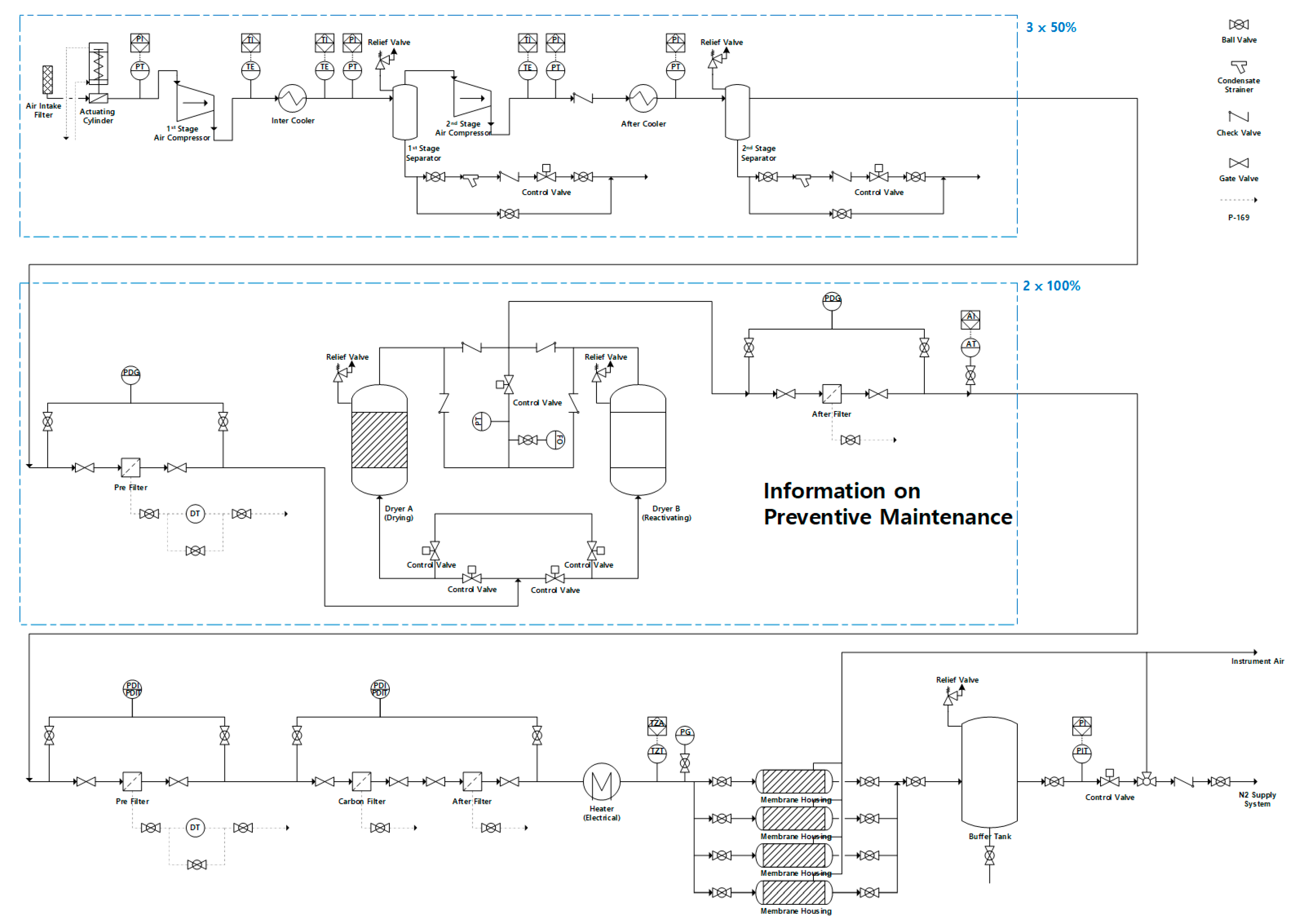
2. Description of Target System

In this study, two systems in LNG-FPSO is selected as a target for the availability estimation. These are air compression and nitrogen generation systems in LNG-FPSO. LNG-FPSO is a huge facility for LNG production in offshore, and its concern has been increased because of the growing demand for LNG. LNG-FPSO is a floating unit for production, processing, storage, and offloading of LNG in remote offshore gas fields. Conventionally, the natural gas in an offshore field is transported by pipeline to onshore for processing. LNG-FPSO does not require the pipeline because it processes the natural gas itself in offshore. It is specialized for small scale gas field. Topside modules of the LNG-FPSO can be categorized into two: a processing module and a utility module. The processing module handles the primary hydrocarbon, whereas the utility module deals with utilities including energy, water, air, and diesel oil. The utility module provides utilities to the processing system for safe and stable operation. Some failure of the utility module can be critical because safety systems for preventing an accident are operated by the utility module.

The topside of LNG-FPSO can be divided into ten modules as shown in Figure 1. A produced feed gas come up through a turret, and it is transported to an inlet facility module. Slug in the feed gas is removed by a slug catcher, and liquid is separated by a separator. CO₂, Hg, and H₂O in the feed gas is removed in a pre-treatment module. The treated natural gas is liquefied by a liquefaction module, and a refrigeration module supplies the refrigerant to the liquefaction module. The heavier components than methane like ethane, butane, and propane are separated by a fractionation module. Some amounts of natural gas are transferred to a fuel gas compression system, and it is utilized for power generation. The liquefied natural gas is stored in storage tanks with LPG and condensate. A condensate stabilizer module separates the relatively light components for safe operation. Condensate is mainly composed of propane, butane, pentane, and heavier hydrocarbon. When condensate contains light components like methane and ethane, it can be vaporized and increase the pressure of a storage tank during storage. These light components should be separated before storage. A blowdown module treats combustion fluids in emergency situations. The utility module supplies various utilities to other modules for the operation.

In this study, air compression and nitrogen generation systems are analyzed in the utility module because those are important systems for stable and safe operation. A general utility module contains an instrument and service air system, a nitrogen generation system, a cooling water system, a seawater system, a hot oil system, a portable water system, a produced and wastewater system, and a diesel oil system. The instrument and service air system compresses the air up to approximately 10 bar for the usage of the instrument and others. The nitrogen generation system supplies nitrogen to the customers. The cooling water system is used to provide the cooling medium for all of the topside modules. The sea water system provides the seawater to various systems. The hot oil system increases the temperature of the oil within a specified range. It utilizes waste heat from flue gas using waste heat recovery units installed in a power generation system. The portable water system distributes water to topside eyewash and safety shower, and hot and cold water for personal usage. The produced and wastewater system removes the oil in the produced water from topside separators. The diesel oil system distributes the diesel oil to customers by transferring and purifying it.

Figure 2 indicates the air compression and nitrogen generation systems. The systems mainly consist of three pieces of equipment; an air compressor, an air dryer, and a nitrogen generator. Air is compressed by the air compressor, and then the small amount of water in the compressed air is dehydrated by the air dryer. The dry air is sent to a customer requiring the instrument air and to the nitrogen generator. The nitrogen generator separates the nitrogen from the dry air.

Figure 3, Figure 4 and Figure 5 show process diagrams with different design stages. Figure 3 is a process flow diagram (PFD) of the air compression and nitrogen generation systems. PFD shows the main equipment in the system. The preliminary process and instrument diagram (P&ID) is indicated in Figure 4 and Figure 5. P&ID includes not only the main equipment but also piping, instrumentation, and control devices. In this study, the piping information is not contained because it is unnecessary for the availability estimation.

The design stage considered in this study are three. The first stage is PFD and the second stage is the preliminary P&ID. The third stage is preliminary P&ID with the information on preventive maintenance.

• Stage I—PFD
• Stage II—Preliminary P&ID
• Stage III—Preliminary P&ID + Information on Preventive Maintenance

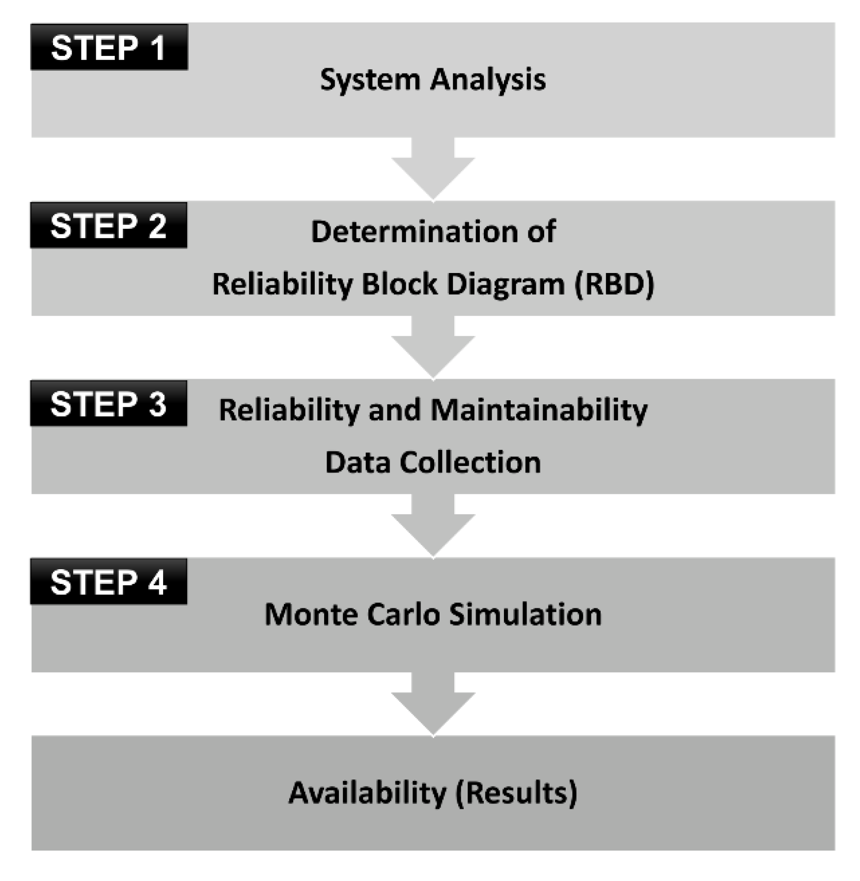
3. Methodology

Several methods are available for the availability estimation: reliability block diagram (RBD), Markov model, and Monte Carlo simulation [17,18]. The former two are an analytical approach whereas the latter one is a simulation approach. The analytical approach calculates the availability using mathematical equations, while the simulation technique estimates it by generating scenarios. When the system is complex, the analytical approaches like RBD and Markov model are unrealistic. They are additionally difficult to apply to the system, which has nonconstant failure and repair rates. However, the Monte Carlo simulation approach can handle inconstant failure/repair rates and multi-state systems. One of the drawbacks of the Monte Carlo simulation is the long simulation time, but it can be overcome by the advanced simulation techniques. In this study, Monte Carlo simulation is employed for the availability estimation.

Figure 6 shows the procedure for the availability estimation using Monte Carlo Simulation. First of all, the target system is analyzed, and then the reliability block diagram is drawn for the modeling of the system. The data for reliability and maintainability is collected from the data sources. The availability of the target system is estimated using the Monte Carlo Simulation. The followings are the details of each step.

3.1. STEP 1 System Analysis

First, the information required for the availability estimation is gathered, and the system is analyzed. The boundary and a level of the system analysis determined in this step. The given operating conditions and assumptions for the availability estimation are determined. Those include the lifespan of the system, number of simulations, distribution function of failure, distribution function of repair time, unit of failure rate, and unit of repair time.

Table 1. Operation conditions and assumption.

Items
Lifespan	20 years
Number of simulations	250
Distribution function of failure	Exponential
Distribution function of repair time	Constant
Unit of failure rate	Number of failure/106 h
Unit of repair time	Hours

tabulates the information.

3.2. STEP 2 Determination of Reliability Block Diagram (RBD)

RBD is a block structure to show success logic of a system. The blocks represent equipment or components of the system to fulfill a specified function. Success path can be visually verified so that it can be easily understood. In this step, the RBD of the system is determined based on Step 1′s results. The followings indicate the RBD with the different design development states.

3.2.1. RBD at Stage I (PFD Stage)

Figure 7 shows the RBD at Stage I. It is divided into three parts as shown in Figure 6: air compression, air dryer, and nitrogen generation parts. The configuration of the air compressor part is 3 × 50%. It means that three compressors are installed, and the capacity of each compressor is 50%. Two compressors are in operation, and one compressor is on standby for a failure of the operating compressors. The air dryer part has 2 × 100% configuration. One air dryer is redundancy. In the nitrogen generation part, the membrane has the 4 × 33% configuration. Three membranes are operated, and the remaining membrane stands by for a failure.

3.2.2. RBD at Stage II (Preliminary P&ID)

Figure 8, Figure 9 and Figure 10 indicate the RBD at Stage II (for the preliminary P&ID stage). Figure 8, Figure 9 and Figure 10 show the RBD for the air compression, air dryer, and nitrogen generation parts, respectively.

3.2.3. RBD at Stage III (Preliminary P&ID + Information on Preventive Maintenance)

RBD at Stage III is almost identical with that for stage II excepting the additional information on preventive maintenance. One block for the preventive maintenance is added for stage III.

3.3. Step 3 Data Collection

The reliability and maintenance data are required for the availability estimation. Since the results of the availability estimation are significantly influenced by the reliability and maintenance data, they are important. Reliability data is linked to the failure rate. The maintenance data is associated with the corrective maintenance time (repair time) and the preventive maintenance time. When the failure occurs, the corrective maintenance is conducted to a system. Preventive maintenance is performed on the basis of maintenance policies and strategies. The data can be categorized into three depending on the kinds of sources: Open data (from open books and reports), vendor data, and in-house data. This study uses the OREDA (Offshore and onshore reliability data) and vendor data. OREDA is offshore and onshore reliability data handbook sponsored by oil and gas companies. It is considered a unique data source in the offshore industry. OREDA is employed in this study because it is the most suitable for it [19,20]. Vendor data is taken from a manufacturer of air compression and nitrogen generation systems.

Table 2. Reliability and maintainability data for air and nitrogen system.

Items	Source	Failure Rate			Active Repair Time
		Lower	Mean	Upper	Mean	Max.
Compressor	OREDA 2009	-	140.84	779.34	15	98
Electric motor	OREDA 2015	0.87	7.52	19.63	16	25
Heat exchanger	OREDA 2015	0.28	64.94	243.9	28	96
Separator	OREDA 2015	0.34	73.49	271.39	6.4	12
Dryer	OREDA 2015	18.32	29.22	44.37	6.2	11
Heater	OREDA 2015	244.7	349.24	484.57	14	84
Membrane	OREDA 2015	18.32	29.22	44.37	6.2	11
Filter	* OREDA 2015	-	4.67	-	1.105	-
Relief valve	OREDA 2015	0.04	2.07	6.41	6.9	13
Check valve	OREDA 2015	0.01	2.47	9.24	2	2
Ball valve (Utilities)	OREDA 2015	2.73	11.65	25.65	5	6
Ball valve (Condensate processing)	OREDA 2015	12.08	72.09	226.9	27	39
Control valve	OREDA 2015	0.99	19.8	93.96	9	9
Gate valve	OREDA 2015	0.04	3.74	12.37	20	72
Control logic unit	OREDA 2015	0.08	17.4	64.59	-	-
Pressure input device	OREDA 2015	0.01	1.09	3.73	7	12
Trap	Vender	-	16.31	22.83	2	-

* This data is regenerated using the component data in Offshore and onshore reliability data (OREDA) 2015.

indicates the reliability and maintenance data employed in this study.

Table 3. Preventive maintenance information on air compression and nitrogen generation systems.

Equipment		Periodic (month)	Maintenance Time (hour)
Air compressor	Component replacement 1	6	0.5
	Component replacement 2	24	3
	Main maintenance	36	72
Air dryer	Component replacement 1	6	0.5
	Component replacement 2	24	1
	Main maintenance	36	24
Nitrogen generator	Component replacement 1	6	0.5
	Component replacement 2	24	1
	Main maintenance	36	24

indicates the information on the preventive maintenance. The preventive maintenance is conducted to prevent unexpected future failure. It is classified into four categories: age-based, clock-based, condition-based, and opportunity maintenance [18]. In the age-based maintenance, the preventive maintenance is performed at the defined age of the system (e.g., the number of take-offs/landings for an airplane). The clock-based maintenance is carried out at specified calendar time so that it is scheduled by administers. In the condition-based maintenance, the preventive maintenance is initiated by measuring condition variables. The opportunity maintenance is carried out when the system is stopped by the other failure. In this study, the clock-based maintenance is taken into account for the preventive maintenance, and the data is collected from the vendor of the air compression and nitrogen generation systems.

3.4. Step 4 Monte Carlo Simulation

Monte Carlo simulation is employed to estimate the availability. Figure 11 shows the flowchart of the Monte Carlo simulation [21]. First of all, components, their states, and their configuration are defined. Moreover, the next transition time for each component is estimated by the random number generation. The transition time is the time when the phase of a component in the system is changed from normal to failure. In this step, the generated random number is converted into a value of time using a conversion method at a cumulative distribution function. Figure 12 shows how the generated random number is transferred to the value of time by the conversion method. The cumulative distribution function for the exponential distribution is indicated in Equation (1).

$$F\left(x\right)=1-e^{-\lambda x}$$

(1)

where λ is the failure rate, and x is a value of time.

$$R=F\left(x\right)=1-e^{-\lambda x}$$

(2)

where R is the random number between 0 and 1. R* is a generated random number between 0 and 1.

The predicted time from the generated random number is shown in Equation (3).

$$x=F^{-1}\left(R\right)=-\frac{1}{\lambda }\ln \left(1-R\right)$$

(3)

The shortest transition time is found among all of the predicted times, and then the system time is changed to the shortest transition time. If the time is shorter than the mission time, the transition times for all component are estimated again. The mission time is total operation time required to the system like lifespan. When the time is longer than the mission time, the system’s availability is calculated. This process is just one simulation. If the number of simulations is lower than the desired number of simulations, the next simulation is repeatedly performed. The desired number of simulations is determined as referring the convergence of results. When a result converges sufficiently, the number of simulations is selected as the desired number of simulations. The desired number of simulations is determined as setting a sufficiently high number of simulations or determining the number of simulations after the initial simulation. When the number of simulations is the same as the desired number of simulations, the average system availability is calculated finally. The average system availability is the result after the last simulation, while the system availability is the result of each simulation.

4. Results and Discussion

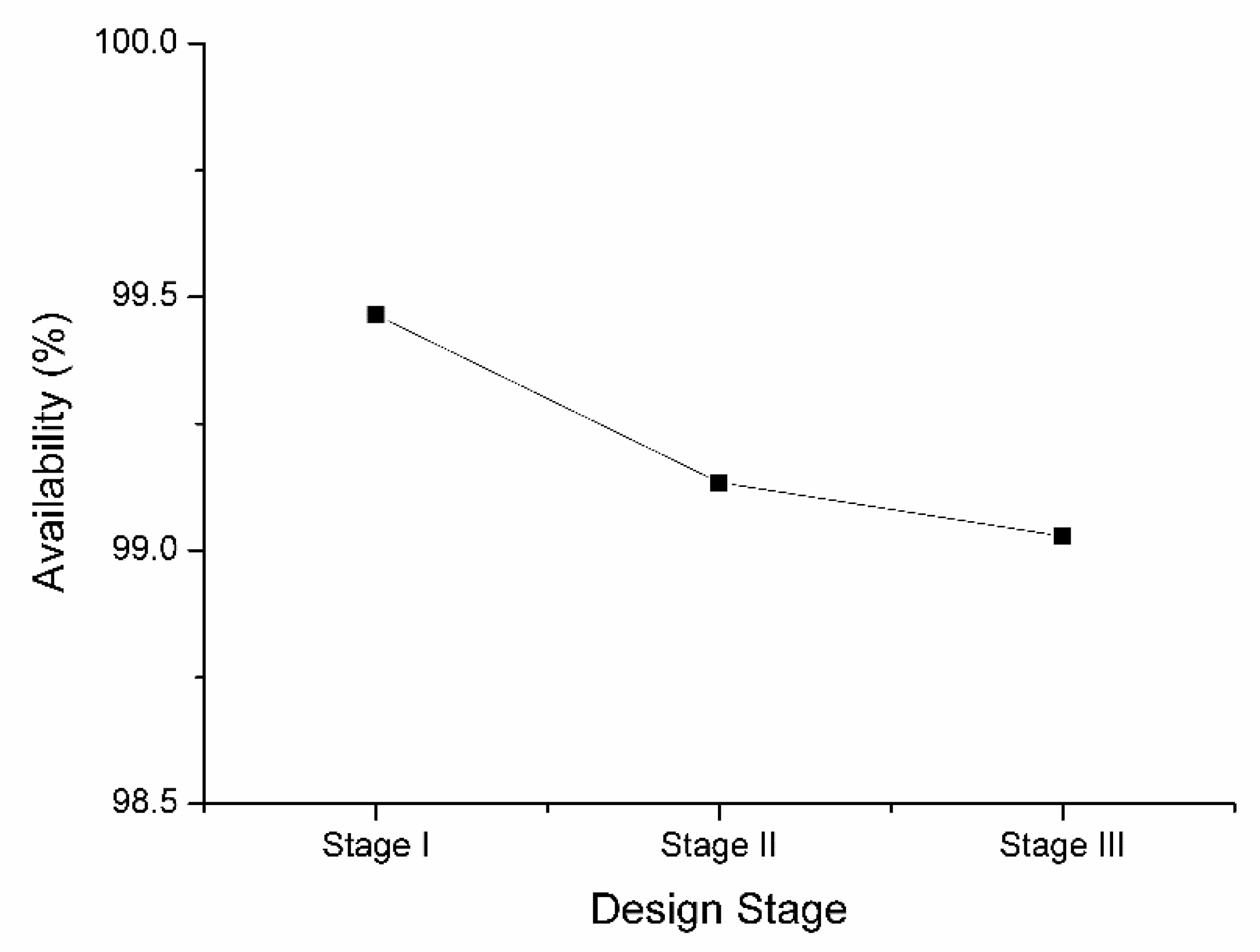
4.1. Availability

Figure 13 shows the availability of the air compression and nitrogen generation systems depending on the design stages. The availability decreased with the increment of the design stages because the system in the late design stage was more complex than that in the early design stage. A complex system has more factors decreasing the availability of the system than a simple system. The availability is decreased by 0.331% when the design stage was changed from Stage I (PFD) to Stage II (P&ID). This meant that the instrument system occupies 0.331% of the system’s availability. When the design stage was transferred from Stage II (P&ID) to Stage III, the availability was decreased by 0.103%. The preventive maintenance influenced about 0.103% of the availability. The availability difference between Stage I and Stage III was 0.434%. It showed that the availability in the early design stage was underestimated compared to the late design stage. The unavailability (1—availability) in the late design stage (0.972%) is approximately 1.8 times severe than that in the early design stage (0.535%). We can predict that the unavailability estimated in the late design stage is 1.8 times serious than that in the early design stage. The availability difference between early and late design stages can be dissimilar with the target system. However, this result provides meaningful information to guess the actual availability in the early design stage.

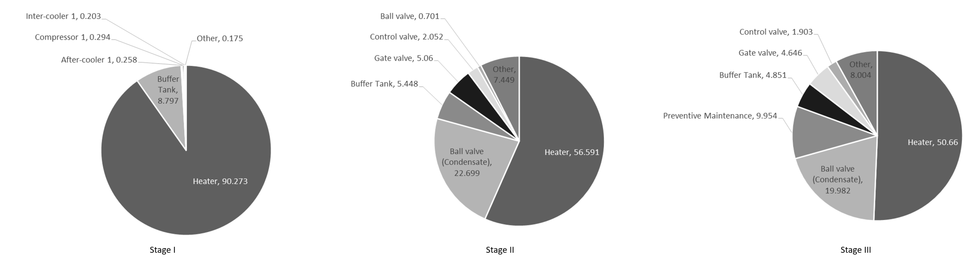
4.2. Component Criticality

Figure 14 shows the component criticality depending on the design stages. The component criticality shows the important component of the availability, and it is the ratio of the component’s failure time to the system failure time. The most crucial component at Stage I was the heater, which accounted for 90.3% criticality. The heater and ball valve (condensate) were critical in Stage II and Stage III. The heater and ball valve (condensate) had 50.7% and 20.0% criticality at the design Stage III, respectively. The preventive maintenance occupied about 10% on the criticality at Stage III. The most critical component was the heater regardless of the design stages. The availability of the system can be significantly increased as installing redundant heaters. The results of the component criticality analysis guide a designer or a decision maker to select additional components to installed to increase availability.

4.3. Sensitivity Analysis

This study performed the sensitivity analysis to investigate the factors affecting the results. It is important to analyze the correlation between the factors and the results because the results can be changed depending on the variation of the factors. In this study, four factors are investigated for the sensitivity analysis: failure rate, repair time, redundant equipment, and modified preventive maintenance schedule. The reliability data used in this study are mainly from OREDA, and its mean value is utilized. The values can be different depending on the target conditions. OREDA predicts the failure rate with 90% confidence interval. The confidence interval describes the amount of uncertainty associated with a sample of a population. The sensitivity analysis was performed for the lower and upper limits of the failure rates. The repair times utilized in this study were also mostly from OREDA. The employed active repair time considers only the time when actual repair work is being done. It does not contain time to shut down the unit, issue the work order, wait for spare parts, start-up after repair. Some variation exists between the active repair time and the actual downtime. (The reason why OREDA only considers the active repair time is that the required time for the preparation and return to the normal operation are different depending on the location of the installation.) The additional repair time is taken into account. The availabilities with and without redundant equipment are estimated to examine its effect on the availability. Finally, the availability is calculated with different preventive maintenance schedules.

4.3.1. Lower amd Upper Failure Rates

Figure 15 indicates the availability depending on the design states with different failure rates: lower, mean, and upper failure rates. As the failure rate was increased from lower to upper, the availability was decreased. In the case of lower and mean failure rates, the availability was slightly decreased with the design stages. In contrast, the availability was significantly reduced in the case of upper failure rate. When the design stage was changed from Stage I (PFD) to Stage II (P&ID), the availability was dramatically decreased in the case of upper failure rate. This indicated that the instrument devices gave a critical impact on the availability. The availabilities are 99.506% (lower) and 97.819% (upper) at Stage III. The upper means that the result is derived using upper failure rate in Table 2, and the lower is the reverse. This meant that the most optimistic availability is 99.506% and the most pessimistic availability is 97.819%.

4.3.2. Additional Repair Time

Figure 16 shows the availability depending on the design stages with the additional repair time. Three additional repair times assumed in this study are 1, 3, and 5 h to investigate the impact of the delayed repair time. The availability decreased with the increment of the repair time. When additional 1, 3, and 5 h were considered at Stage III, the availabilities were 98.969%, 98.823%, and 98.701%, respectively. This result presented that one additional hour in the repair time decreased the availability by 0.065%.

4.3.3. Installation of Redundant Heater

Figure 17 presents the availability depending on the design stages with the installation of the redundant heater. As mentioned in Section 4.1, the most critical component in the availability was the heater regardless of the design stages. The availability was estimated depending on the installation of the redundant heater or not. The availability was considerably increased when the redundant heater is installed. The availability is 99.028% without the redundant heater at Stage III, whereas it is 99.514% with the redundant heater. That is, the redundant heater increased the availability by 0.486%. Although 0.486% availability seems to be low, it is not a negligible value in the system (LNG-FPSO).

4.3.4. Modified Preventive Maintenance Schedule

Figure 18 shows the availability depending on the design stages with the modified preventive maintenance. As mentioned in Section 3, the preventive maintenance is conducted to prevent the critical failures. There are various activities for the preventive maintenance as indicated in Table 3. These activities are individually conducted depending on their inherent periodic. When the activities have different schedule, some activities can be merged to increase the availability. Although simultaneous preventive maintenance increases the availability, it requires new engineers to conduct the activities at the same time. Since all components have the same preventive maintenance schedule, different schedules were assumed in the modified schedule. The result showed that the availability was decreased by 0.076% through the modified preventive maintenance schedule. Since the preventive maintenance was not considered at Stages I and II, the values at those stages were unchanged.

5. Conclusions

This study estimated the availability of air and nitrogen systems depending on the design stages to analyze the gap between early and late design stages. Three design stages were considered: Stages I–III. Stage I was the process flow diagram (PFD) stage and Stage II was the piping and instrument diagram (P&ID) stage. In Stage III, the preventive maintenance was additionally considered comparing to Stage II. The Monte Carlo simulation approach was employed for the availability estimation. The results presented that the availabilities were decreased with the design progress. It is obvious because the system was more complex with the design development. The availability difference between Stage I and Stage II was 0.331%, and that was 0.103% between Stage II and Stage III. These indicated that the instrument system and the preventive maintenance occupied 0.331% and 0.103%, respectively. This result also presented that the availability in the early design stage (Stage I) was underestimated compared to the late design stage (Stage III). The unavailability at the late design stage was 1.8 times higher than the early design stage. We could guess the availability at the late design stage using the result at the initial design stage. The most critical component in the air and nitrogen systems was the heater regardless of design stages. The sensitivity analysis was conducted to analyze the key factors on the results. The most crucial factor was the redundant equipment. When the redundant heater was installed, the availability was increased by 0.486% at Stage III. The factors for the modified maintenance schedule and additional repair time (1 h) were not significant in the system compared to other factors. Since this study investigated only two systems (air and nitrogen systems) among lots of systems in LNG-FPSO, future studies are required for the whole system (LNG-FPSO). Although this study did not consider the whole system (LNG-FPSO), this gives the important guide to progress the next step for the accurate availability estimation in the early design stage.

References

1. British Standards Institution (BSI). BS 4778-3.1:1991 Quality Vocabulary: Part 3: Availability, Reliability and Maintainability Terms, Section 3.1 Guide to Concepts and Related Definitions; BSI: London, UK, 1991. [Google Scholar]
2. Basker, B.; Martin, P. Availability prediction by using a method of simulation. Microelectron. Reliab. 1977, 16, 135–141. [Google Scholar] [CrossRef]
3. Keller, A.; Stipho, N. Availability studies of two similar chlorine production plant. Reliab. Eng. 1981, 2, 271–281. [Google Scholar] [CrossRef]
4. Bosman, M. Availability analysis of a natural gas compressor plant. Reliab. Eng. 1985, 11, 13–26. [Google Scholar] [CrossRef]
5. Aven, T. Availability evaluation of oil/gas production and transportation systems. Reliab. Eng. 1987, 18, 35–44. [Google Scholar] [CrossRef]
6. Khan, M.R.; Kabir, A.Z. Availability simulation of an ammonia plant. Reliab. Eng. Syst. Saf. 1995, 48, 217–227. [Google Scholar] [CrossRef]
7. Hajeeh, M.; Chaudhuri, D. Reliability and availability assessment of reverse osmosis. Desalination 2000, 130, 185–192. [Google Scholar] [CrossRef]
8. Zio, E.; Baraldi, P.; Patelli, E. Assessment of the availability of an o shore installation by Monte Carlo simulation. Int. J. Press. Vessels Pip. 2006, 83, 312–320. [Google Scholar] [CrossRef]
9. Crespo, A.; Heguedas, A.S.; Iung, B. Monte Carlo-based assessment of system availability. A case study for cogeneration plants. Reliab. Eng. Syst. Saf. 2005, 88, 273–289. [Google Scholar] [CrossRef]
10. Michelassi, C.; Monaci, G. Availability assessment of a raw gas re-injection plant for the production of oil and gas. In Proceedings of the 16th IMEKO TC4 International Symposium Exploring New Frontiers of Instrumentation and Methods for Electrical and Electronic Measurements, Florence, Italy, 22–24 September 2008; pp. 777–783. [Google Scholar]
11. Chang, D.; Rhee, T.; Nam, K.; Chang, K.; Lee, D.; Jeong, S. A study on availability and safety of new propulsion systems for LNG carriers. Reliab. Eng. Syst. Saf. 2008, 93, 1877–1885. [Google Scholar] [CrossRef]
12. Görkemli, L.; Ulusoy, S.K. Fuzzy Bayesian reliability and availability analysis of production systems. Comput. Ind. Eng. 2010, 59, 690–696. [Google Scholar] [CrossRef]
13. Seo, Y.; You, H.; Lee, S.; Huh, C.; Chang, D. Evaluation of CO2 liquefaction processes for ship-based carbon capture and storage (CCS) in terms of life cycle cost (LCC) considering availability. Int. J. Greenh. Gas Control. 2015, 35, 1–12. [Google Scholar] [CrossRef]
14. Seo, S.; Chu, B.; Noh, Y.; Jang, W.; Lee, S.; Seo, Y.; Chang, D. An economic evaluation of operating expenditures for LNG fuel gas supply systems onboard ocean-going ships considering availability. Ships Offshore Struct. 2014, 11, 213–223. [Google Scholar] [CrossRef]
15. Gowid, S.; Dixon, R.; Ghani, S. Profitability, reliability and condition based monitoring of LNG floating platforms: A review. J. Nat. Gas Sci. Eng. 2015, 27, 1495–1511. [Google Scholar] [CrossRef] [Green Version]
16. Hwang, H.; Lee, J.-H.; Hwang, J.; Jun, H.-B. A study of the development of a condition-based maintenance system for an LNG FPSO. Ocean Eng. 2018, 164, 604–615. [Google Scholar] [CrossRef]
17. Verma, A.K.; Srividya, A.; Karanki, D.R. Reliability and Safety Engineering; Springer: London, UK, 2010; ISBN 978-1-84996-231-5. [Google Scholar]
18. Rausand, M.; Høyland, A. System Reliability Theory: Models, Statistical Methods, and Applications, 2nd ed.; John Wiley & Sons, Inc.: Hoboken, NJ, USA, 2004; ISBN 0-7803-3274-1. [Google Scholar]
19. Oreda Project. OREDA: Participants Offshore Reliability Data Hand-Book, 5th ed.; DNV: Oslo, Norway, 2009; ISBN 8214027055. [Google Scholar]
20. Oreda Project. OREDA: Participants Offshore and Onshore Reliability Data Handbook, 6th ed.; DNV GL: Oslo, Norway, 2015. [Google Scholar]
21. Seo, Y.; Han, S.; Kang, K.; Noh, H.-J.; Park, S.; Jung, J.-Y.; Chang, D.; Čepin, M.; Briš, R. Availability estimation of utility module in offshore plant depending on system configuration. In Advances and Trends in Engineering Sciences and Technologies II; Al Ali, M., Platko, P., Eds.; CRC Press: London, UK, 2017; pp. 2195–2202. [Google Scholar]
Figure 1. Topside modules of liquefied natural gas—floating production storage and offloading unit (LNG-FPSO).
Applsci 10 08657 g001
Figure 2. Block diagram of air and nitrogen systems.
Applsci 10 08657 g002
Figure 3. Process flow diagram (PFD) of air and nitrogen system.
Applsci 10 08657 g003
Figure 4. The preliminary process and instrument diagram (P&ID) of air and nitrogen system.
Applsci 10 08657 g004
Figure 5. P&ID of air and nitrogen system with information on preventive maintenance.
Applsci 10 08657 g005
Figure 6. Procedure for availability estimation using Monte Carlo simulation.
Applsci 10 08657 g006
Figure 7. Reliability block diagram at Stage I (PFD stage).
Applsci 10 08657 g007
Figure 8. Reliability block diagram at Stage II (preliminary P&ID stage)—Air compression part.
Applsci 10 08657 g008
Figure 9. Reliability block diagram at Stage II (preliminary P&ID stage)—Air dryer part.
Applsci 10 08657 g009
Figure 10. Reliability block diagram at Stage II (preliminary P&ID stage)—Nitrogen generation part.
Applsci 10 08657 g010
Figure 11. Procedure for availability estimation using Monte Carlo simulation [21].
Applsci 10 08657 g011
Figure 12. Conversion method to transfer random number to value of time at cumulative distribution.
Applsci 10 08657 g012
Figure 13. Availability depending on the stages.
Applsci 10 08657 g013
Figure 14. Component criticality depending on the stages.
Applsci 10 08657 g014
Figure 15. Availability with different failure rate.
Applsci 10 08657 g015
Figure 16. Availability with additional repair time.
Applsci 10 08657 g016
Figure 17. Availability with installation of redundant heater.
Applsci 10 08657 g017
Figure 18. Availability with modified preventive maintenance schedule.
Applsci 10 08657 g018