On the Influence of Reference Mahalanobis Distance Space for Quality Classification of Complex Metal Parts Using Vibrations

Abstract

Mahalanobis distance (MD) is a well-known metric in multivariate analysis to separate groups or populations. In the context of the Mahalanobis-Taguchi system (MTS), a set of normal observations are used to obtain their MD values and construct a reference Mahalanobis distance space, for which a suitable classification threshold can then be introduced to classify new observations as normal/abnormal. Aiming at enhancing the performance of feature screening and threshold determination in MTS, the authors have recently proposed an integrated Mahalanobis classification system (IMCS) algorithm with robust classification performance. However, the reference MD space considered in either MTS or IMCS is only based on normal samples. In this paper, an investigation on the influence of the reference MD space based on a set of (i) normal samples, (ii) abnormal samples, and (iii) both normal and abnormal samples for classification is performed. The potential of using an alternative MD space is evaluated for sorting complex metallic parts, i.e., good/bad structural quality, based on their broadband vibrational spectra. Results are discussed for a sparse and imbalanced experimental case study of complex-shaped metallic turbine blades with various damage types; a rich and balanced numerical case study of dogbone-cylinders is also considered.

1. Introduction

The Mahalanobis–Taguchi system (MTS) is a powerful tool for studying multidimensional systems developed by Genichi Taguchi [1,2,3]. MD and Taguchi robust engineering are effectively integrated and applied to the diagnosis and prediction of multivariate data. Due to its effectiveness and easy operation without any underlying statistical assumptions, this method has been widely used in various applications such as product quality testing systems, mechanical fault diagnoses, financial early-warnings, medical diagnoses, and other fields [4,5,6,7].

MTS is a pattern recognition system that employs the concepts of orthogonal arrays (OAs) and signal-to-noise ratios (SNRs) to screen useful features. The feature selection process, however, is seen as not optimal by several scholars [8,9,10]. Therefore, some scholars have carried out in-depth and extensive research and have achieved promising results, making important contributions to the development of MTS [11,12,13,14,15,16,17]. The majority of those methodologies are based on metaheuristic algorithms such as the genetic algorithm (GA), binary particle swarm optimization (BPSO), binary ant colony optimization (BACO), and the binary gravitational search algorithm (BGSA), effectively improving the feature selection strategy.

Another challenge to implementing MTS in practice is the determination of a suitable threshold for distinguishing between normal and abnormal observations. Taguchi [18] proposed a quadratic loss function (QLF) to determine the classification threshold, but this is unrealistic because it is difficult to estimate the relative cost or loss in reality. A simpler and more practical approach using the Chebyshev theorem, called the “probability threshold method”, has been proposed [19]. There is also a substantial body of qualitative research in developing threshold determination methods [20,21,22].

A novel two-stage Mahalanobis classification system (MCS), as well as its integrated version (IMCS), has been recently proposed by the current authors [16,17]. IMCS integrates the decision boundary searching process, which is based on the particle swarm optimizer algorithm, directly into the feature selection phase (based on BPSO or BGSA) for constructing the MD space. Compared to classical MTS, both MCS and IMCS showed improved classification performance for sorting (i.e., good/bad structural quality) complex metal parts based on their vibrational response [17].

The primary objective of this paper is to investigate the influence of the reference MD space on the classification performance of the recently proposed IMCS classifier [17]. The reference MD space is constructed by considering (i) normal samples, (ii) abnormal samples, and (iii) both normal and abnormal samples. In addition, the impact of an imbalanced dataset on classification accuracy is also discussed. This paper is organized into five sections. Section 2 presents the concept of multidimensional MD space. The procedure of IMCS with three different reference MD spaces is demonstrated in Section 3, followed by an experimental case study on complex-shaped metallic turbine blades and a numerical study on dogbone cylinders in Section 4. Section 5 gives the conclusions of this paper.

2. Multidimensional Mahalanobis Distance

The M-dimensional ($M\ge 1$) multivariate system is considered. Samples from normal observations (healthy samples) are defined as $x_{ij}^k$, indicating the $j$th variable of the $i$th normal observation in the $k$th dimension $\left(i=1,2,\dots ,n;j=1,2,\dots ,p;k=1,2,\dots ,M\right)$.

The samples are firstly standardized as

$$z_{ij}^k=\frac{x_{ij}^k-{\overline{x}}_j^k}{{\mathrm{s}}_j^k}$$

(1)

In Equation (1), ${\overline{x}}_j^k$ and ${\mathrm{s}}_j^k$ represent the mean and standard deviation of the $j$th variable in the $k$th dimension.

Then, $M$-dimensional MD values can be obtained as

$$\begin{array}{c}\mathit{M}{\mathit{D}}_i=\left[M{D}_i^1,M{D}_i^2,\dots ,M{D}_i^M\right]\\ M{D}_i^k=\frac{1}{p}{\mathit{Z}}_i^k{}^T{\mathit{R}}^k{}^{-1}{\mathit{Z}}_i^k\\ \left(i=1,2,\dots ,n;k=1,2,\dots ,M\right)\end{array}$$

(2)

where ${\mathit{Z}}_i^k={\left[z_{i1}^k,z_{i2}^k,\dots ,z_{ip}^k\right]}^T$ and ${\mathit{R}}^k=\frac{1}{n-1}{\sum }_{i=1}^n{\mathit{Z}}_i^k{}^T{\mathit{Z}}_i^k$.

Thereby, MD values for abnormal observations (defective samples) can then be calculated based on the obtained outcomes of ${\mathit{R}}^k$ from Equation (2).

3. Methodology

3.1. Integrated Mahalanobis Classification System (IMCS)

The current authors have recently proposed the IMCS algorithm [17], which is an extension of the earlier proposed two-stage MCS approach [16] for improving classification performance. The IMCS approach incorporates the decision-making process directly into the feature selection process, thus avoiding the need for extra user-dependent inputs and enhancing classification performance. The framework of IMCS is presented in Figure 1.

The procedure of IMCS can be briefly summarized as follows. The original dataset, comprising n samples with p variables, is firstly randomly split into training and testing sets. In the training stage, the optimal feature subset can be screened out under the objective to maximize the classification accuracy max($\frac{TP+TN}{TP+FP+TN+FN}$) (TP: true positive; TN: true negative; FP: false positive; FN: false negative) in MD space in the training dataset using the binary particle swarm optimizer (BPSO) algorithm [23,24]. A PSO-based classifier is introduced to accomplish classification decision threshold optimization, updating itself simultaneously with the BPSO-based feature selection process at each iteration. In the case of multidimensional MD space, alternative decision boundary searching algorithms such as support vector machine (SVM) [25,26], random forest [27,28], and neural network (NN) [29,30] can be easily considered in the IMCS algorithm. Finally, the optimal features and classification threshold extracted from the training dataset are used to make predictions on the testing dataset. In order to avoid overfitting for sparse training datasets, the cross-validation of k-folders is considered. The downside of this fully integrated MCS approach is the higher computational effort needed compared to two-stage MCS [16].

3.2. Construction of Reference MD Space

MD space is essentially the distance between an unknown data point and a given population, indicating the similarity between them. The construction of a good reference MD space is crucial in order to obtain good classification performance. For instance, the reference MD space in MTS is constructed on the basis of a supervised learning process, using a given set of normal observations. A threshold to distinguish the two classes is then properly defined and used to classify the unknown samples. If the observed MD is less than the threshold, the unknown sample has statistically similar characteristics to the normal population of the samples.

The main objective of this paper is to investigate the potential of constructing the reference MD space not only by considering normal samples but also abnormal samples, as well as a combination of them. Three different thresholds will be introduced based on three different reference MD spaces. Classification performance on the testing dataset is then compared and evaluated for these three different MD spaces.

The three different classification scenarios are schematically presented in Figure 2. Figure 2a illustrates MD values based on a reference MD space that is constructed by considering only normal observations. The green triangles and red circles represent normal and abnormal observations, respectively. By introducing a suitable decision threshold, indicated as a blue dashed line, the two categories (normal/abnormal) of the given samples can be differentiated. Figure 2b presents the classification scenario by employing a reference MD space that considers only abnormal observations. Scenario 3, shown in Figure 2c, employs a reference MD space that is constructed by using both normal and abnormal observations. As such, this approach enables us to introduce a two-dimensional linear decision boundary.

In the following context, $M{D}^{normal}$ and $M{D}^{abnormal}$ stand for the Mahalanobis distance based on normal and abnormal observations, respectively.

4. Case Studies

The behavior of the IMCS classifier based on the three different reference MD spaces is evaluated for two different case studies in the field of quality assessment of complex metal parts based on vibrations.

In this paper, symbolic conventions are adopted to represent the structure of the classification procedure: ${\mathbf{IMCS}}_{\mathbf{Y}}^{\mathbf{X}}$ → IMCS indicates the integrated Mahalanobis classification system that employs optimizer X to screen the key features and approach Y to search for the optimal threshold boundary.

4.1. An Experimental Case Study on Complex-Shaped Metallic Turbine Blades

A case study of first-stage turbine blades with complex geometry and internal cooling channels, consisting of 193 healthy and 39 defective blades (see Figure 3), is presented in this section. The blades have been labeled as good/bad using alternative inspection procedures (e.g., X-ray Computed Tomography, ultrasonic, penetrant testing, microscopic sectioning, operational performance, and operator experience). For more details on the turbine blades, readers are referred to [16].

The frequency response functions (FRFs) of these blades are measured by Vibrant Corporation (link: www.vibrantndt.com) using the process-compensated resonant test (PCRT) technique in the frequency range of 3–38 kHz. PCRT is a nondestructive testing technology for the vibrational testing of parts. A schematic of the PCRT procedure is displayed in Figure 4. The test part (a turbine blade in this case) is supported by three piezoelectric transducers that are positioned in a fixture. One transducer acts as an actuator and excites a broadband sweep sine signal. The remaining two transducers are used to monitor the vibrational response signal. In this regard, PCRT is implemented as a single input multiple output (SIMO) test. Based on the measured FRFs, important features such as resonance frequencies and their associated damping ratios and amplitudes can then be estimated. These features are used in a classification algorithm, which is based on a learning process, in order to discriminate between good and bad parts.

Figure 5 displays FRFs from two healthy samples and one defective sample. A significant difference can be observed between them. Based on the measured FRFs, 15 stable resonance frequencies have been extracted, which serve as the feature set for the ${\mathbf{IMCS}}_{\mathbf{PSO}}^{\mathbf{BPSO}}$ algorithm.

A training pool comprises 60% of the original dataset. The training pool itself consists of a 60% training dataset and a 40% validation dataset, randomly selected from healthy and defective samples in equal proportions. The remaining 40% of the original dataset is the testing dataset (blind parts) and is used to evaluate the classification performance of the trained algorithm. Thus, the numbers of the training dataset, the validation dataset, and the testing dataset are 87, 52, and 93, respectively. For BPSO, the maximum iteration number is T = 100, and the number of particles in the BPSO is set to N = 10. A 5-folder cross-validation is considered.

All programs are implemented in the platform MATLAB2018b^® (laptop with Intel^® Core™ i7-8650U processor (4 cores) up to 4.20 GHz and RAM 32GB).

4.1.1. Reference MD Space Based on Healthy Samples

First, the turbine blades are classified with the IMCS algorithm by considering a reference MD space that is constructed based on the healthy samples.

Among the initial 15 features (resonance frequencies extracted from FRFs), only 6 out of 15 features are screened: $f_2,f_4,f_5,f_8,f_{14},f_{15}$ ≈ (5.9, 9.6, 10.7, 19.8, 25.9, 36.0) kHz.

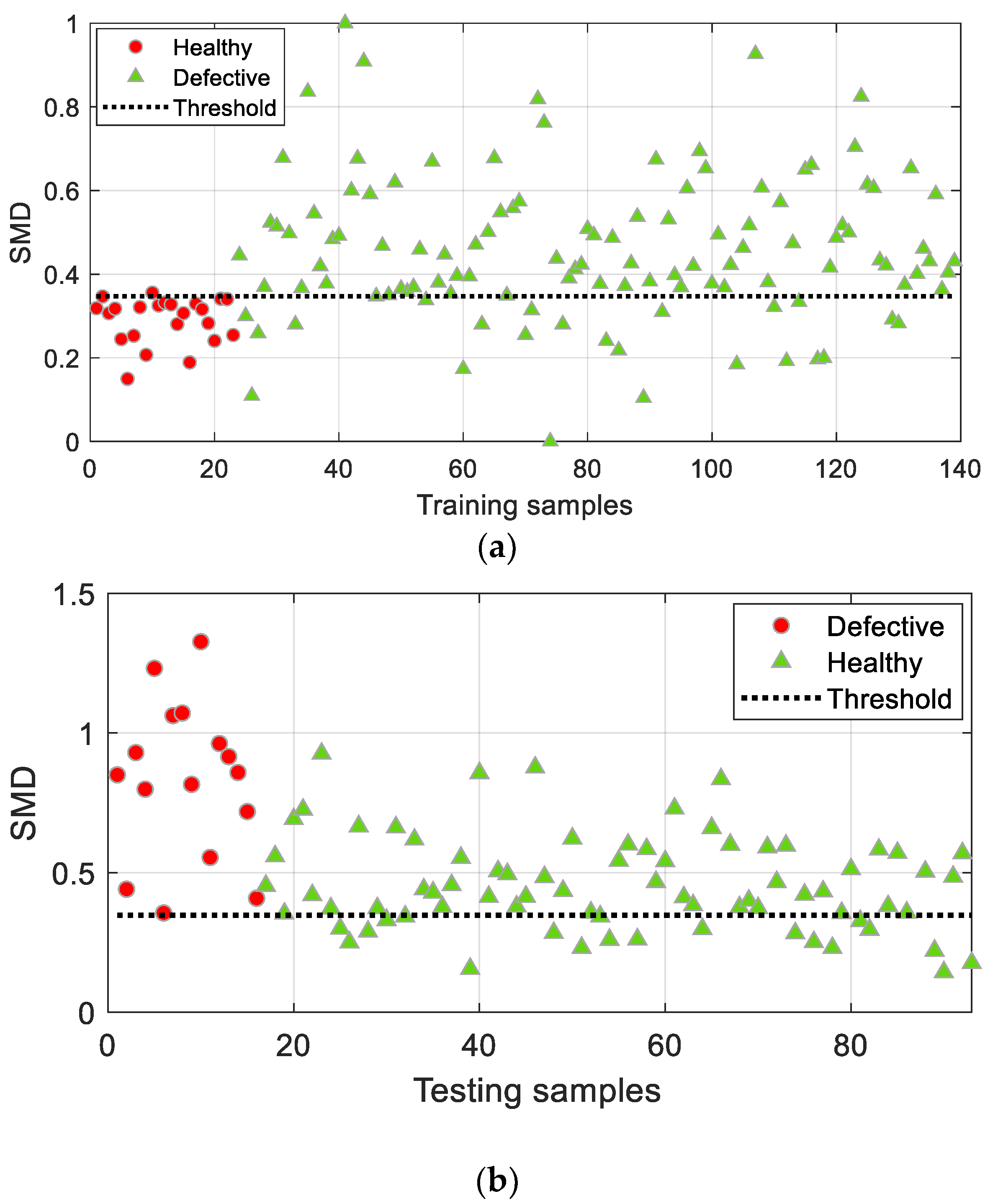
The classification results are shown in Figure 6, where the misclassifications are marked with black blocks. SMD (scaled Mahalanobis distance) in Figure 6 stands for the scaled Mahalanobis distance, which is obtained by considering a logarithmic normalization, as follows:

$$SMD\_training=\frac{log\left(M{D}^{training}\right)-min\left(log\left(M{D}^{training}\right)\right)}{max\left(log\left(M{D}^{training}\right)\right)-min\left(log\left(M{D}^{training}\right)\right)}$$

(3)

$$SMD\_testing=\frac{log\left(M{D}^{testing}\right)-min\left(log\left(M{D}^{training}\right)\right)}{max\left(log\left(M{D}^{training}\right)\right)-min\left(log\left(M{D}^{training}\right)\right)}$$

(4)

The procedure was run 20 times, independently, and the average accuracy and standard deviation of classification results are summarized in

Table 1. Classification performance of the algorithm over 20 independent runs using a reference MD space based on healthy samples.

	Training Accuracy (%)	Testing Accuracy (%)	Number of Features (–)
${\mathbf{IMCS}}_{\mathbf{PSO}}^{\mathbf{BPSO}}$	98.81 ± 0.39	97.06 ± 1.35	5.50 ± 0.73

. IMCS achieved accuracies of 96.40% and 96.77% for the training pool dataset and testing dataset, respectively. Note that a small value of standard deviation and a relatively large standard deviation can be observed in training and testing accuracy, respectively, reflecting the discrepancy between the populations of the training and testing samples due to the sparse dataset.

4.1.2. Reference MD Space Based on Defective Samples

Another perspective in classification is to construct a reference MD space based on defective samples. The same configuration as the dataset allocation in Section 4.1.1 is adopted here. The classification criteria, in essence, are to differentiate between the healthy and defective samples by evaluating their similarity to the defective population (rather than to the healthy population, as in Section 4.1).

The classification results are shown in Figure 7 for the training and testing datasets.

The IMCS algorithm shows 82.73% and 62.37% classification accuracies for training and testing datasets, respectively. There are seven screened features $f_1,f_3,f_5,f_7,f_{12},f_{13},f_{14}$ ≈ (3.9, 7.0, 10.7, 19.1, 24.5, 25.5, 25.9) kHz. The results clearly indicate that constructing an MD space based on defective samples deteriorates the classification performance significantly. The immediate reason behind this observation is found in the high sensitivity of MD to even slight variations [31]. Furthermore, there are various kinds of defects in the first-stage turbine blades, such as (i) microstructure changes due to overheating, (ii) airfoiled cracking, and (iii) intergranular erosion (corrosion) [16]. Additionally, each of these defect types may vary at different MD levels and, as such, different distributions. This obviously makes it difficult to construct a good reference MD space in which the MD population is well clustered. A further challenge arises from the fact that the number of defective samples is too sparse in the feature space to construct a good reference MD space.

Classification performance using IMCS over 20 independent runs is summarized in

Table 2. Classification performance of the algorithm over 20 independent runs using a reference MD space based on defective samples.

	Training Accuracy (%)	Testing Accuracy (%)	Number of Features (–)
${\mathbf{IMCS}}_{\mathbf{PSO}}^{\mathbf{BPSO}}$	87.20 ± 9.29	79.46 ± 10.11	5.33 ± 2.90

. Apart from the low mean values of accuracies, the standard deviation increased significantly, indicating poor classification performance.

4.1.3. Reference MD Space Based on Healthy and Defective Samples

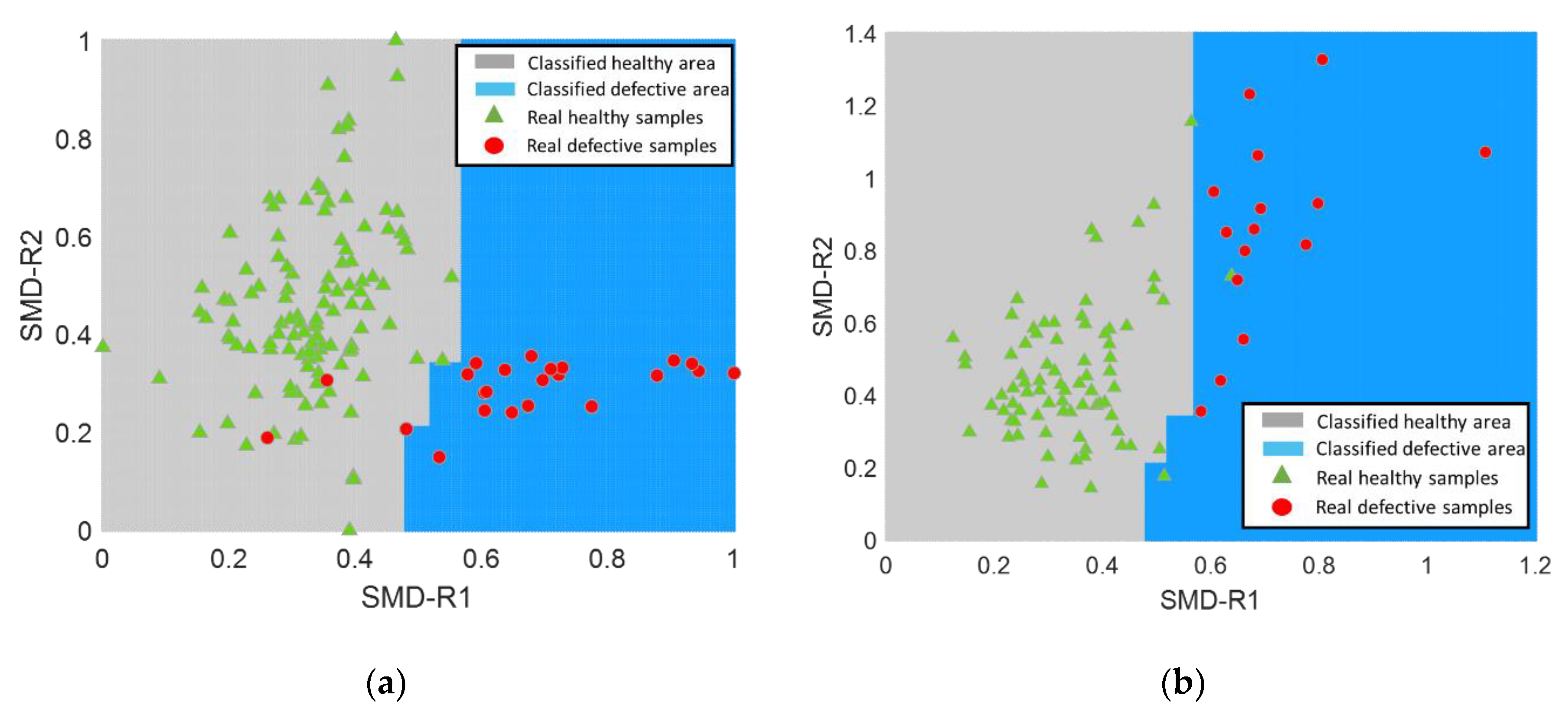
From the above results, it may be concluded that the use of defective samples to construct MD space has to be avoided. In this section, a two-dimensional reference MD space is constructed on the basis of both healthy and defective samples, partitioning the MD space into four regions of interest by two linear thresholds, threshold 1 and threshold 2. These two thresholds are learned from the IMCS classifier based on a reference MD space constructed from healthy samples and defective samples, respectively. The classification results of training and testing datasets are shown in Figure 6, where SMD-R1 and SMD-R2 stand for SMD based on the reference MD space constructed by healthy samples and defective samples, respectively.

The four areas are referred to as A1, A2, A3, and A4 in Figure 8, providing insight into the reliability of the classification. Areas A1 and A2 indicate “high” reliability, and areas A3 and A4 indicate “low” reliability. Notably, the samples located in area A1 are all correctly classified as healthy samples. Moreover, most of the misclassifications appear in the areas with “low” reliability. Although there is no specific contribution in terms of classification accuracy by considering a two-dimensional MD space, further insight into the classified samples can be gained from the divided areas with different credibility.

A significant drop in classification accuracy observed in both training and testing datasets from

Table 3. Classification performance of ${\mathbf{IMCS}}_{\mathbf{PSO}}^{\mathbf{BPSO}}$ over 20 independent runs using a reference MD space based on both healthy and defective samples.

	Training Accuracy (%)	Testing Accuracy (%)	Number of Features (–)
${\mathbf{IMCS}}_{\mathbf{PSO}}^{\mathbf{BPSO}}$	90.12 ± 1.22	80.58 ± 2.81	SMD-R1: 5.50 ± 0.73 SMD-R2: 5.33 ± 2.90

is associated with the two introduced linear thresholds, partitioning the two-dimensional MD space into healthy (A1) and defective (A2, A3, A4) regions.

From a more technical point of view, the linear thresholds may pose a strict restriction in classification accuracy. Instead of using linear threshold boundaries, a nonlinear classification boundary is considered to reach maximal discrimination between classes. Random forest (RF) is employed, which is an ensemble classifier composed of multiple decision trees [32]. RF consists of a set of simple tree predictors, in which each predictor can respond to a set of predicted scores. By combining multiple weak classifiers, the final classification scores are voted or averaged. Because of this, RF can yield good classification performance, with high generalization capability; at the same time, it is less sensitive to overfitting issues. In this study, the RF model was built and trained by generating an ensemble of 20 bagged classification trees. The training process was implemented in MATLAB@ by using the Statistics and Machine Learning toolbox. The training and prediction outcomes, considering the RF approach for threshold determination, are displayed in Figure 9.

Classification accuracies of 98.56% and 97.85% were obtained for the training data and testing data, respectively. Compared to the results using the reference MD space based on healthy samples in Section 4.1.1, a classification accuracy quantifies the same percentage of samples being correctly identified in the testing dataset. However, this is referred to as the result of a single trial and cannot be generalized. Thus, statistical classification results of 20 independent runs based on the RF technique are summarized in

Table 4. Classification performance of the random forest (RF) technique over 20 independent runs.

	Training Accuracy (%)	Testing Accuracy (%)	Number of Features (–)
${\mathbf{IMCS}}_{\mathbf{RF}}^{\mathbf{BPSO}}$	99.93 ± 0.22	97.31 ± 0.81	SMD-R1: 5.50 ± 0.73 SMD-R2: 5.33 ± 2.90

.

A clear enhancement can be found for ${\mathbf{IMCS}}_{\mathbf{RF}}^{\mathbf{BPSO}}$ (SMD-R1+SMD-R2), compared to ${\mathbf{IMCS}}_{\mathbf{PSO}}^{\mathbf{BPSO}}$ (SMD-R1+SMD-R2), due to the use of nonlinear decision boundaries. However, comparing ${\mathbf{IMCS}}_{\mathbf{RF}}^{\mathbf{BPSO}}$ (SMD-R1+SMD-R2) with the classifier constructed with a reference MD space based on healthy samples only (i.e., ${\mathbf{IMCS}}_{\mathbf{PSO}}^{\mathbf{BPSO}}$ (SMD-R1)) indicates only a marginal enhancement in training and testing accuracy.

4.2. A Numerical Case Study on a Synthetic Dataset of Cylinders

Due to the sparsity and imbalance of the experimental dataset in Section 4.1, the active role of alternating the reference MD space may not be manifested sufficiently. Another case study based on a rich synthetic dataset of dogbone cylinders, composed of 3562 samples, is provided by Vibrant Corporation (link: www.vibrantndt.com) and further discussed in this section. They are modeled as nickel, single-crystal, cylindrical (tapered to gauge section) dogbones (see Figure 10) using the finite element method.

Two key determinants of the physical conditions of these cylinders are creep (inelastic deformation) and θ (crystal orientation, relative to the long axis of the dogbone). The variations of creep and θ are simulated in the ranges 0–9.9% and 0–37.9, respectively. Moreover, the feature database is generated by extracting the resonance frequencies in the bandwidth 3–190 kHz.

Damaged parts are defined as creep >0.5%; θ > 10, resulting in a balanced dataset of 1857 healthy samples and 1750 defective samples.

First, the whole dataset is split into a training pool and a testing set with the proportion 3:7, where the training pool is further composed of training and validation sets with the proportion 6:4. In the ${\mathbf{IMCS}}_{\mathbf{PSO}}^{\mathbf{BPSO}}$ procedure, the maximum iteration number T for the BPSO algorithm is set as 200 and the number of particles is set to N = 20. A 5-folder validation is used to train the classifier.

4.2.1. Reference MD Space Based on Healthy Samples

Figure 11 presents the classification results of ${\mathbf{IMCS}}_{\mathbf{PSO}}^{\mathbf{BPSO}}$ for the training pool dataset and testing dataset, with an accuracy of 99.06% and 98.68%, respectively.

It is worth remembering that the feature dimension has been significantly reduced from 44 to only 9, which is conducive to the processing of big data. The screened features are listed in

Table 5. Classification performance of the algorithms based on difference MD spaces over 20 independent runs.

	Training Accuracy (%)	Testing Accuracy (%)	Number of Features (–)
${\mathbf{IMCS}}_{\mathbf{PSO}}^{\mathbf{BPSO}}$ (SMD-R1)	99.43 ± 0.14	98.81 ± 0.24	8.00 ± 1.63
${\mathbf{IMCS}}_{\mathbf{PSO}}^{\mathbf{BPSO}}$ (SMD-R2)	92.58 ± 0.46	92.35 ± 0.91	2.10 ± 0.32
${\mathbf{IMCS}}_{\mathbf{PSO}}^{\mathbf{BPSO}}$ (SMD-R1+SMD-R2)	98.23 ± 0.36	98.15 ± 0.51	SMD-R1: 8.00 ± 1.63 SMD-R2: 2.10 ± 0.32
${\mathbf{IMCS}}_{\mathbf{RF}}^{\mathbf{BPSO}}$ (SMD-R1+SMD-R2)	99.93 ± 0.07	99.02 ± 0.20	SMD-R1: 8.00 ± 1.63 SMD-R2: 2.10 ± 0.32

.

4.2.2. Reference MD Space Based on Defective Samples

This subsection offers an additional perspective on the classification performance of the synthetic dataset based on a reference MD space constructed by defective samples only.

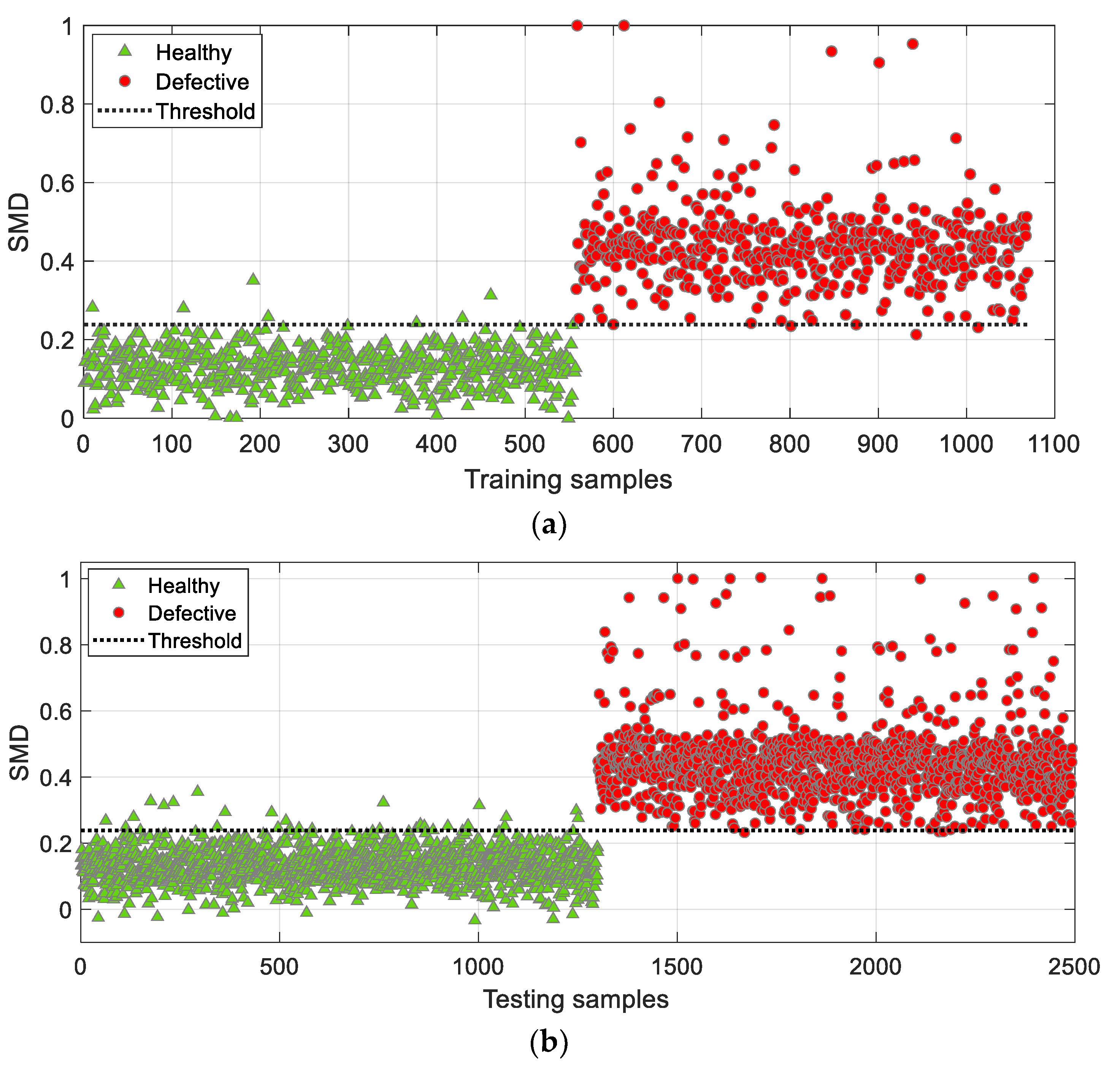
Classification results of the training and testing datasets, shown in Figure 12, are inferior to the results obtained in Section 4.2.1, with an accuracy of 93.10% and 92.33%, respectively.

As it can be observed from Figure 12, the SMD values of the defective samples are spatially dispersed in the entire SMD space [0,1]. Alternatively, the SMD values of healthy samples are highly concentrated in the range of 0.6–0.7. It can be interpreted by the fact that the resonance frequencies in defective samples vary greatly, thus yielding a large variation in MD as well. This also offers a good understanding of the obtained concentrated SMD values for healthy samples due to the small variations in resonance frequencies among healthy samples. Although the presented classification results are not completely satisfactory compared to the results in Section 4.2.1, it further provides an additional opportunity to explore the in-depth study by constructing a two-dimensional SMD space in which both reference MD spaces can be examined.

4.2.3. Reference MD Space Based on Healthy and Defective Samples

A two-dimensional MD space is constructed using the reference MD space based on both healthy and defective samples. Similar to Section 4.1.3, the constructed MD space is divided into four regions in terms of reliability by two linear thresholds.

The two overlapping areas covered by the two thresholds are A1 and A2 as healthy area and defective area, respectively. Therefore, the identified points located within the areas A1 and A2 are considered highly reliable. As can be seen from the classification results presented in Figure 13, almost all the samples in the areas A1 and A2 are correctly identified. Thus, enhancing the classification accuracy in the less reliable areas of A3 and A4 by considering the use of a nonlinear boundary is of great significance.

Combining the obtained two-dimensional SMDs (SMD-R1 and SMD-R2) in an RF-based classifier further increases the classification accuracies to 99.63% and 99.16% for the training and testing datasets, respectively. The classification results of training and testing samples are presented in Figure 14. It is worth noting that the entire two-dimensional MD space is clearly divided into two areas based on a nonlinear boundary—Green (healthy) and Blue (defective)—instead of the four areas in Figure 13.

To obtain an average classification result for the three different scenarios, 20 independent runs for each were performed. The mean values and standard deviations for training accuracy, testing accuracy, and the number of screened features are summarized in Table 4 below. Interestingly, only an average value of two features is filtered for SMD-R2, implying the significant impact induced by the change of reference MD space. A slight decline of accuracy can be found using ${\mathbf{IMCS}}_{\mathbf{PSO}}^{\mathbf{BPSO}}$ (SMD-R1+SMD-R2) compared to ${\mathbf{IMCS}}_{\mathbf{PSO}}^{\mathbf{BPSO}}$ (SMD-R1); this is due to the weak identifiability of the two areas of A3 and A4. Thus, the introduction of a two-dimensional nonlinear boundary enables us to maximize classification performance. A mean value of 99.02% ± 0.20 on the testing samples was obtained using ${\mathbf{IMCS}}_{\mathbf{RF}}^{\mathbf{BPSO}}$ (SMD-R1+SMD-R2).

4.3. Additional Investigations on the Synthetic Dataset

Benefiting from the substantial amount of synthetic dogbone cylinders, it was possible to further explore the robustness and ability of the proposed IMCS algorithm to handle an imbalanced dataset.

4.3.1. The Robustness of the IMCS Algorithm

To evaluate the robustness of the proposed IMCS algorithm, classification accuracy is obtained through a dynamic feature selection scheme. The basic idea is to run the IMCS process for several rounds and exclude the features that were selected in the previous round from the next round in order to observe the impact of different feature subsets on classification performance.

In this subsection, the training and testing datasets used in Section 4.2 are adopted. A total of five rounds was run. In each round, IMCS classifiers based on the reference MD space constructed from healthy samples (SMD-R1), defective samples (SMD-R2), and both SMD-R1 and SMD-R2 are considered.

The classification accuracies of the testing dataset, based on the reference MD space constructed from healthy samples, defective samples, and both healthy and defective samples, are reported in Figure 15 for the five consecutive rounds. Considering that the most promising features are selected first, it is clear that subsequent rounds will yield lower classification accuracies. This can be clearly seen in Figure 15.

Furthermore, the result indicates that the ${\mathrm{IMCS}}_{\mathrm{RF}}^{\mathrm{BPSO}}$ classifier with the reference MD space of both healthy and defected parts (SMD-R1 + SMD-R2) consistently exhibits the highest accuracies over the five rounds, followed by the ${\mathrm{IMCS}}_{\mathrm{PSO}}^{\mathrm{BPSO}}$ classifier with the reference MD space of healthy parts (SMD-R1) and, finally, the ${\mathrm{IMCS}}_{\mathrm{PSO}}^{\mathrm{BPSO}}$ classifier with the reference MD space of defected parts (SMD-R2), with the lowest accuracies in all rounds.

4.3.2. Imbalanced Dataset

An imbalanced dataset usually refers to classification problems where the number of observations for each category is not equal [33,34]. To investigate the impact of an imbalanced dataset on classification performance, four additional scenarios are conducted in this subsection. The training pool is randomly selected as 30% of the original dataset.

Scenario 1: Training pool consists of healthy/defective samples with a ratio of 1:10

Scenario 2: Training pool consists of healthy/defective samples with a ratio of 3:7

Scenario 3: Training pool consists of healthy/defective samples with a ratio of 5:5

Scenario 4: Training pool consists of healthy/defective samples with a ratio of 7:3

Scenario 5: Training pool consists of healthy/defective samples with a ratio of 10:1

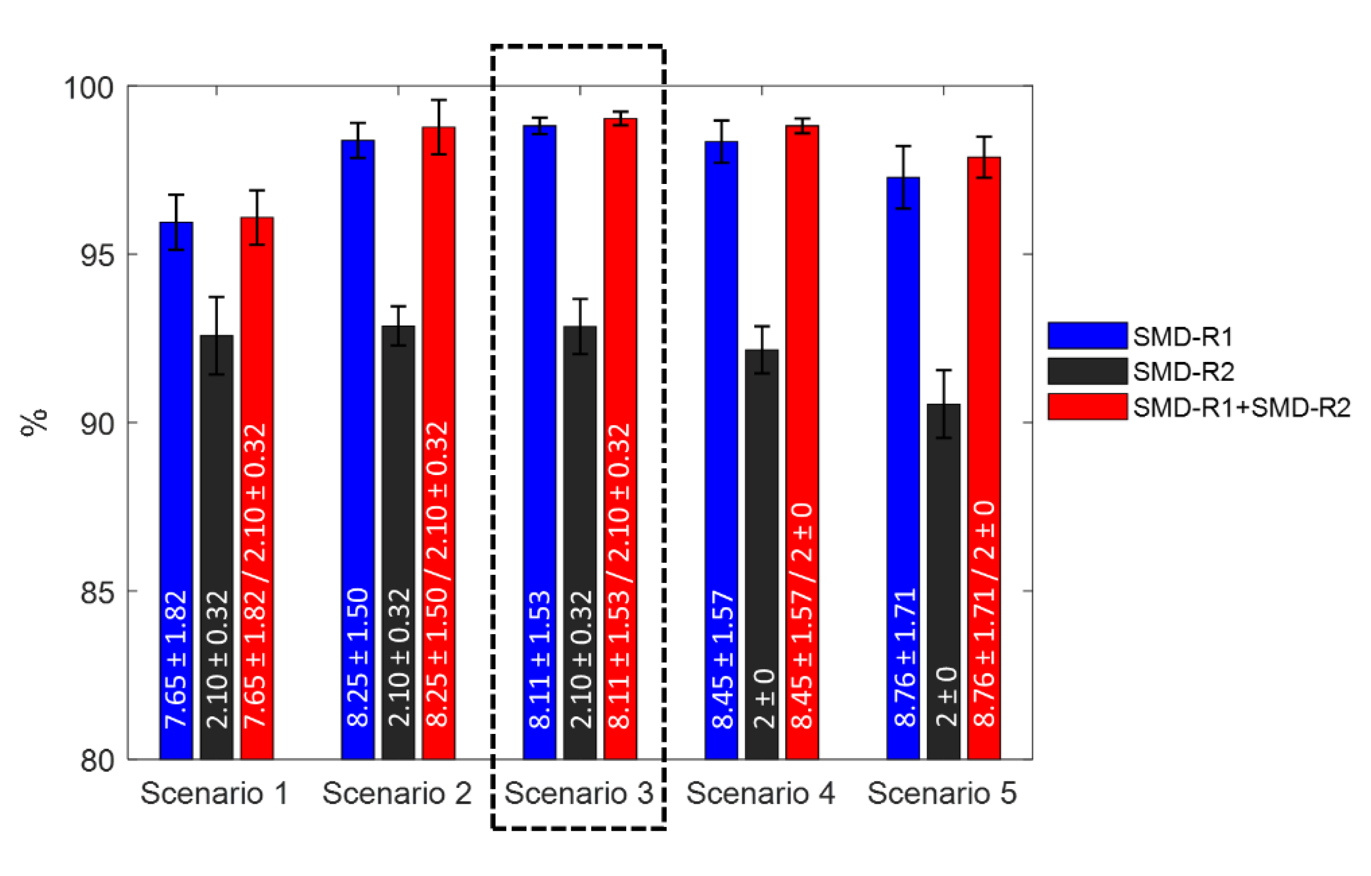
Similarly, such random sampling is performed over 20 independent runs for each scenario in order to evaluate the average classification ability of the method. The detailed classification results under the five scenarios are listed in Figure 16, indicating their overall accuracies (mean ± std). Additionally, the numbers on the bars stand for the overall number of selected features using the form of mean ± std.

Of the five scenarios, the ${\mathrm{IMCS}}_{\mathrm{RF}}^{\mathrm{BPSO}}$ classifier (SMD-R1 + SMD-R2) demonstrates the optimal classification performance for both training and testing datasets. Using a balanced classification ratio of 5:5 in Scenario 3, marked by a black-dashed rectangular, the highest testing accuracy was obtained based on the ${\mathrm{IMCS}}_{\mathrm{RF}}^{\mathrm{BPSO}}$ classifier, followed by slightly imbalanced cases (Scenario 4 and Scenario 2). Scenario 1, with a severe imbalanced ratio of 1:10, revealed the worst results, with an overall testing accuracy of 96.09%.

Of additional interest is that training accuracy based on the ${\mathrm{IMCS}}_{\mathrm{PSO}}^{\mathrm{BPSO}}$ classifier (SMD-R2) was gradually improved with an increase in the proportion of healthy samples. In fact, the direct cause of this phenomenon is the decrease of variation diversity of MD in MD space due to the reduction in the proportion of defective samples. However, even in this case, it does not necessarily contribute to the accuracy of the testing dataset.

The discussion of the impact of an imbalanced classification ratio indicates that the increase of an imbalanced ratio in training data sets indeed reduces testing accuracy. In particular, the classification could be worse if the imbalance weight is heavily skewed towards the defective samples.

However, the above discussion on the classification performance of an imbalanced dataset is based on the condition that sufficient samples are available. For a sparse dataset, such as the turbine blades in Section 4.1, the imbalance is still challenging.

5. Conclusions

This paper provides a different perspective on the classification performance of the recently proposed integrated Mahalanobis classification system (IMCS) by considering different reference MD spaces. The reference MD spaces were constructed by considering (i) only normal observations (corresponds to the classical approach), (ii) only abnormal observations, and (iii) a combination of both normal and abnormal observations.

A sparse and imbalanced experimental case study of metal turbine blades with complex shapes was conducted, showing marginal improvements in employing an alternative reference MD space.

An additional rich and balanced synthetic dataset of dogbone cylinders was also studied in order to further exploit the ability to deal with imbalanced dataset cases and to investigate the robustness of the IMCS approach.

The results demonstrate that the achieved classification accuracy is far from satisfactory if the reference MD space is based on only defective samples. An appealing classification result was obtained using IMCS based on a reference MD space constructed from both healthy and defected samples. A further investigation on bringing in the nonlinear classification boundary from random forest indicates an improvement to classification performance. For imbalanced datasets, the classification accuracy of the testing dataset decreases as the imbalance of the training dataset increases. To note, IMCS with a reference MD space based on both healthy and damaged samples eventually yields better classification performance for imbalanced datasets.

References

- Taguchi, G.; Rafanelli, A.J. Taguchi on Robust Technology Development: Bringing Quality Engineering Upstream; ASME Press: New York, NY, USA, 1994. [Google Scholar]
- Taguchi, G.; Jugulum, R. The Mahalanobis-Taguchi Strategy: A Pattern Technology System; John Wiley & Sons: New York, NY, USA, 2002. [Google Scholar]
- Taguchi, G.; Chowdhury, S.; Taguchi, S. Robust Engineering: Learn how to Boost Quality While Reducing Costs & Time to Market; McGraw-Hill Professional Pub: New York, NY, USA, 2000. [Google Scholar]
- Kalantari, M.; Rabbani, M.; Ebadian, M. A decision support system for order acceptance/rejection in hybrid MTS/MTO production systems. Appl. Math. Model. 2011, 35, 1363–1377. [Google Scholar] [CrossRef]
- Soylemezoglu, A.; Jagannathan, S.; Saygin, C. Mahalanobis Taguchi system (MTS) as a prognostics tool for rolling element bearing failures. J. Manuf. Sci. Eng. 2010, 132, 051014. [Google Scholar] [CrossRef]
- Lee, Y.C.; Teng, H.L. Predicting the financial crisis by Mahalanobis-Taguchi system—Examples of Taiwan’s electronic sector. Expert Syst. Appl. 2009, 36, 7469–7478. [Google Scholar] [CrossRef]
- Taguchi, G.; Rajesh, J. New trends in multivariate diagnosis. Sankhyā Indian J. Stat. Ser. B 2000, 62, 233–248. [Google Scholar]
- Friedman, J.H.; Silverman, B.W. Flexible parsimonious smoothing and additive modeling. Technometrics 1989, 31, 3–21. [Google Scholar] [CrossRef]
- Woodall, W.H.; Koudelik, R.; Tsui, K.L.; Kim, S.B.; Stoumbos, Z.G.; Carvounis, C.P. A review and analysis of the Mahalanobis—Taguchi system. Technometrics 2003, 45, 1–15. [Google Scholar] [CrossRef]
- Pal, A.; Maiti, J. Development of a hybrid methodology for dimensionality reduction in Mahalanobis–Taguchi system using Mahalanobis distance and binary particle swarm optimization. Expert Syst. Appl. 2010, 37, 1286–1293. [Google Scholar] [CrossRef]
- Reséndiz-Flores, E.O.; Navarro-Acosta, J.A.; Hernández-Martínez, A. Optimal feature selection in industrial foam injection processes using hybrid binary Particle Swarm Optimization and Gravitational Search Algorithm in the Mahalanobis–Taguchi System. Soft Comput. 2020, 24, 341–349. [Google Scholar] [CrossRef]
- ReséNdiz, E.; Rull-Flores, C.A. Mahalanobis–Taguchi system applied to variable selection in automotive pedals components using Gompertz binary particle swarm optimization. Expert Syst. Appl. 2013, 40, 2361–2365. [Google Scholar] [CrossRef]
- Reséndiz, E.; Moncayo-Martínez, L.A.; Solís, G. Binary ant colony optimization applied to variable screening in the Mahalanobis-Taguchi system. Expert Syst. Appl. 2013, 40, 634–637. [Google Scholar] [CrossRef]
- El-Banna, M. A novel approach for classifying imbalance welding data: Mahalanobis genetic algorithm (MGA). Int. J. Adv. Manuf. Technol. 2015, 77, 407–425. [Google Scholar] [CrossRef]
- Ramlie, F.; Jamaludin, K.R.; Dolah, R.; Muhamad, W.Z.A.W. Optimal feature selection of taguchi character recognition in the mahalanobis-taguchi system using bees algorithm. Glob. J. Pure Appl. Math. 2016, 12, 2651–2671. [Google Scholar]
- Cheng, L.; Yaghoubi, V.; Van Paepegem, W.; Kersemans, M. Mahalanobis classification system (MCS) integrated with binary particle swarm optimization for robust quality classification of complex metallic turbine blades. Mech. Syst. Signal Process. 2020, 146, 107060. [Google Scholar] [CrossRef]
- Cheng, L.; Yaghoubi, V.; Van Paepegem, W.; Kersemans, M. Quality inspection of complex-shaped metal parts by vibrations and an integrated Mahalanobis classification system (IMCS). Struct. Health Monit. (Forthcoming). [CrossRef]
- Taguchi, G.; Wu, Y. Introduction to Off-Line Quality Control; Central Japan Quality Control Association: Tokyo, Japan, 1979. [Google Scholar]
- Su, C.T.; Hsiao, Y.H. An evaluation of the robustness of MTS for imbalanced data. IEEE Trans. Knowl. Data Eng. 2007, 19, 1321–1332. [Google Scholar] [CrossRef]
- Huang, C.L.; Chen, Y.H.; Wan, T.L.J. The Mahalanobis Taguchi System—Adaptive resonance theory neural network algorithm for dynamic product designs. J. Inf. Optim. Sci. 2012, 33, 623–635. [Google Scholar] [CrossRef]
- Kumar, S.; Chow, T.W.; Pecht, M. Approach to fault identification for electronic products using Mahalanobis distance. IEEE Trans. Instrum. Meas. 2009, 59, 2055–2064. [Google Scholar] [CrossRef]
- El-Banna, M. Modified Mahalanobis Taguchi system for imbalance data classification. Comput. Intell. Neurosci. 2017, 2017. [Google Scholar] [CrossRef]
- Eberhart, R.; Kennedy, J. Particle swarm optimization. In Proceedings of the IEEE International Conference on Neural Networks, University of Western Australia, Perth, Western Australia, 27 November–1 December 1995; Volume 4, pp. 1942–1948. [Google Scholar]
- Kennedy, J.; Eberhart, R.C. A discrete binary version of the particle swarm algorithm. In Proceedings of the IEEE International Conference on Systems, Man, and Cybernetics. Computational Cybernetics and Simulation, Orlando, FL, USA, 12–15 October 1997; Volume 5, pp. 4104–4108. [Google Scholar]
- Schlkopf, B.; Smola, A.J.; Bach, F. Learning with Kernels: Support Vector Machines, Regularization, Optimization, and Beyond; The MIT Press: Cambridge, MA, USA, 2018. [Google Scholar]
- Nalepa, J.; Kawulok, M. Selecting training sets for support vector machines: A review. Artif. Intell. Rev. 2019, 52, 857–900. [Google Scholar] [CrossRef]
- Speiser, J.L.; Miller, M.E.; Tooze, J.; Ip, E. A comparison of random forest variable selection methods for classification prediction modeling. Expert Syst. Appl. 2019, 134, 93–101. [Google Scholar] [CrossRef]
- Shaikhina, T.; Lowe, D.; Daga, S.; Briggs, D.; Higgins, R.; Khovanova, N. Decision tree and random forest models for outcome prediction in antibody incompatible kidney transplantation. Biomed. Signal Process. Control 2019, 52, 456–462. [Google Scholar] [CrossRef]
- Hecht-Nielsen, R. Theory of the backpropagation neural network. In Neural Networks for Perception; Academic Press: Cambridge, MA, USA, 1992; pp. 65–93. [Google Scholar]
- Dheir, I.M.; Mettleq, A.S.A.; Elsharif, A.A.; Abu-Naser, S.S. Classifying nuts types using convolutional neural network. Int. J. Acad. Inf. Syst. Res. 2020, 3, 12–18. [Google Scholar]
- Werner, M. Identification of Multivariate Outliers in Large Data Sets. Ph.D. Thesis, University of Colorado, Denver, CO, USA, 2003. [Google Scholar]
- Liaw, A.; Wiener, M. Classification and regression by randomForest. R News 2002, 2, 18–22. [Google Scholar]
- Haixiang, G.; Yijing, L.; Shang, J.; Mingyun, G.; Yuanyue, H.; Bing, G. Learning from class-imbalanced data: Review of methods and applications. Expert Syst. Appl. 2017, 73, 220–239. [Google Scholar] [CrossRef]
- Fernández, A.; García, S.; Galar, M.; Prati, R.C.; Krawczyk, B.; Herrera, F. Learning from Imbalanced Data Sets; Springer: Berlin, Germany, 2018; pp. 1–377. [Google Scholar]
Figure 1.
The schematic of the integrated Mahalanobis classification system (IMCS) algorithm.
Figure 2.
Three different classification scenarios, listed as (a) reference MD space based on ; (b) reference MD space based on ; (c) reference MD space based on both and .
Figure 3.
(a) Generic model of the turbine blade; (b) sectional drawing of the turbine blade.
Figure 4.
A schematic of the measurement procedure (reproduced with permission from Elsevier) [
16].
Figure 5.
Frequency response functions (FRFs) of two healthy samples and one defective sample.
Figure 6.
(a) Classification on training pool dataset; (b) classification on the testing dataset.
Figure 7.
(a) Classification on the training dataset; (b) classification on the testing dataset.
Figure 8.
Figure 9.
(a) -based classification on the training dataset; (b) -based classification on the testing dataset.
Figure 10.
A generic model of the cylinder.
Figure 11.
Figure 12.
Figure 13.
Figure 14.
Figure 15.
Testing accuracy on the testing dataset for five consecutive rounds, with dynamic feature selection over 20 independent runs.
Figure 16.
Classification results on the testing dataset for 5 scenarios.